

1. Introduction
Antarctic ice shelves are of great importance for the dynamics of the entire Antarctic ice sheet, because they drain, to a large extent, the coastward mass flux of the inland ice via a relatively small number of fast-moving ice streams and outlet glaciers (e.g. Reference Bamber, Vaughan and JoughinBamber and others, 2000). Ice shelves are supposed to be sensitive elements of the climate system, since their dynamics depend on physical quantities (e.g. ice surface and ocean temperatures) which are directly affected by climate change.
The interactions between ice shelves and the ocean determine the sub-shelf water properties and thus play an important role in regional ocean dynamics. It is therefore important to understand the dynamics of ice shelves, how they react to conditions such as thickness and temperature distribution, boundary conditions from inland ice inflow, outflow to the ocean at the front, and grounded areas and rifts.
The disintegration and retreat of seven ice shelves along the Antarctic Peninsula (Reference Doake and VaughanDoake and Vaughan, 1991a,b; Reference SkvarcaSkvarca, 1993; Reference WardWard, 1995; Reference Doake, Corr, Rott, Skvarca and YoungDoake and others, 1998; Reference Rott, Rack, Nagler and SkvarcaRott and others, 1998, Reference Rott, Rack, Skvarca and De Angelis2002; Reference Skvarca, Rack and RottSkvarca and others, 1999; Reference Fox and VaughanFox and Vaughan, 2005) and the recent break-up events on Wilkins Ice Shelf (Reference Braun, Humbert and MollBraun and others, 2008; Reference Humbert and BraunHumbert and Braun, 2009) demonstrate the potential of ice shelves to become unstable. Since ice shelves buttress adjacent glaciers and ice streams, their disintegration leads to an increase in the discharge of inland ice. Evidence for increased glacier velocity has been obtained by means of remote sensing by Reference De Angelis and SkvarcaDe Angelis and Skvarca (2003), Reference Rignot, Casassa, Gogineni, Krabill, Rivera and ThomasRignot and others (2004) and Reference Scambos, Bohlander, Shuman and SkvarcaScambos and others (2004) in areas where ice shelves have disintegrated in previous years.
The ability to predict the temporal variability of ice dynamics is limited, because boundary parameters (e.g. melt rates) at the ice/ocean interface are difficult to obtain. Therefore, it is crucial to gain understanding of their current dynamics through diagnostic simulations. The aim of this study is to perform numerical simulations using two models describing ice-shelf flow dynamics, to make detailed comparisons using these different simulations and to test the effects of model design on the flow regime of dynamically important damage zones like rifts and shear zones.
2. Study Area
The Brunt Ice Shelf (BIS)/Stancomb-Wills Ice Tongue (SWIT) system is characterized as a thin unbounded ice shelf (Fig. 1a) with an area of ∼27 950 km2. It is attached to Caird Coast, Coats Land, East Antarctica, at the eastern margin of the Weddell Sea. The geographical position is 73.9–76.0° S, 18.4–27.5° W.

Fig. 1. (a) Map of the Brunt Ice Shelf study region including feature names. Underlain is a Mosaic of Antarctica (MOA) image acquired between late 2003 and early 2004. Sea ice is found in the Weddell Sea off McDonald Ice Rumples. PB stands for Precious Bay, and BI for Bakewell Island. The inset shows the location in the eastern Weddell Sea, Antarctica. (b) The location of rifts 1 and 2. The bold gray curve indicates non-vanishing inflow speeds, while the thick black curve corresponds to zero inflow. The thin curve represents the boundary condition calving front. Arrows denote the direction and magnitude of the prescribed inflow speeds.
The BIS–SWIT system differs from other ice shelves in that the BIS and SWIT are linked by a discontinuous mass of icebergs bound together by a melange of extraordinarily thick fast ice (up to 50 m), covered by a thick accumulated snow layer, and smaller meteoric ice blocks (personal communication from C.S.M. Doake, 2002).
Stancomb-Wills Ice Stream enters the ice shelf in the northeastern part from Caird Coast with a velocity of ∼750 m a−1 (Reference GrayGray, 2001). This ice stream forms a fast-flowing floating ice tongue that is connected with the Riiser-Larsen Ice Shelf (RLIS) on the eastern side, separated by Lyddan Island, a substantial ice rise. According to our own analysis of surface topography data (see below), the thickness of the ice tongue exceeds 450 m at the grounding line and is reduced towards the ice front to ∼200 m (Fig. 2).
The southwestern part of the BIS–SWIT system terminates at Precious Bay (PB), where the thin and slow-moving Brunt Ice Shelf is located. Its ice thickness varies between 100 and 250 m.
There are two major ice rises, Lyddan Island (74.25° S, 20.45° W) and the McDonald Ice Rumples (75.47° S, 26.30° W, which are an ice rise despite the name); a minor ice rise at the ice front east of Lyddan Island, Bakewell Island (BI); and three very small nameless ice rises in the RLIS, close to the grounding line along Princess Martha Coast.
The BIS–SWIT area has been subject to a combined modeling/remote-sensing study by Reference Hulbe, Johnston, Joughin and ScambosHulbe and others (2005). They used a finite-element flow model that is based on the same equations as used in the University of Münster
(MS) model, described in detail below. Reference Hulbe, Johnston, Joughin and ScambosHulbe and others (2005) investigated the effect on ice-shelf velocity of a range of possible combinations of flow-rate factors for regions of ice-thickness contrasts between sea ice and meteoric ice, and various assumptions of the sea-ice thickness. The main difference between their study and the present work is that we focus on the comparison of different realizations of rift zones. Furthermore, the gridded ice-thickness and ice-surface elevation datasets, and the ice-flow velocities across the grounding line used in our study are different.
3. The Ice-Shelf Models
3.1. The Darmstadt model (DA)
Using a general, continuum-mechanical approach, a thermodynamically consistent theory for ice-shelf flow was derived at the Darmstadt University of Technology, Germany, by Reference Weis, Greve and HutterWeis and others (1999) and Reference WeisWeis (2001). It consists of a set of vertically integrated equations for the zeroth order of the shallow-shelf approximation (SSA). The deformation of ice is modeled using Glen’s flow law (Reference GlenGlen, 1958):
where D = sym grad (v) is the strain-rate tensor (symmetric part of the gradient of the velocity v = (vx
, vy
, vz
)), t
D is the Cauchy stress deviator, ![]() is the effective stress, n is the power-law exponent and A(T,W) is the flow-rate factor which contains the dependencies on temperature, T, and water content, W. The flow-enhancement factor, E, parameterizes all other physical contributions such as ice impurities, anisotropy and grain size. The equations of motion for the horizontal velocity (vx
, vy
) in Cartesian coordinates are:
is the effective stress, n is the power-law exponent and A(T,W) is the flow-rate factor which contains the dependencies on temperature, T, and water content, W. The flow-enhancement factor, E, parameterizes all other physical contributions such as ice impurities, anisotropy and grain size. The equations of motion for the horizontal velocity (vx
, vy
) in Cartesian coordinates are:
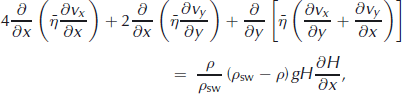

where the coordinates x and y span the horizontal plane, ![]() is the depth-integrated viscosity, ρ is the mean density of meteoric ice (850 kg m−3 over the entire thickness) and ρ
sw is the density of sea water (1028 kg m−3). The depth-integrated viscosity is given by
is the depth-integrated viscosity, ρ is the mean density of meteoric ice (850 kg m−3 over the entire thickness) and ρ
sw is the density of sea water (1028 kg m−3). The depth-integrated viscosity is given by

where z is positive upward, E s = E −1/n is the stress-enhancement factor, B(T , W) = [A(T , W)]−1/n is the associated rate factor, h s is the ice-surface elevation and h b is the depth of the ice-shelf base (ice/ocean interface). Both h s and h b are taken relative to the mean sea level, and the ice thickness is H = h s − h b. Further,

denotes the effective strain rate (second invariant of the strain-rate tensor).
The elliptic system of differential equations (Equations (2) and (3)) is subject to two different types of boundary conditions: (1) prescribed inflow of ice along the grounding line from the adjacent inland ice and (2) the vertically integrated stress-boundary conditions:


at the calving front, which result from balancing the stresses in the ice and the hydrostatic sea-water pressure (nx and ny are the components of the normal unit vector which points away from the ice shelf).
In this study, the horizontal flow field will only be computed diagnostically for present-day conditions. Consequently, the ice-thickness distribution, H(x, y), and the temperature field, T (x, y, z), must also be prescribed. The latter is required for computing the associated rate factor, B(T). Alternatively, the associated rate factor can be prescribed directly, and this approach is actually chosen here.
These equations have been successfully applied to the Ross Ice Shelf (Reference HumbertHumbert, 2005; Reference HumbertHumbert and others, 2005) and Fimbulisen (Reference HumbertHumbert, 2006) in a more sophisticated approach than we use here. The equations have been ported to the commercial finite-element software COMSOL, a high performance finite-element solver for stationary and non-stationary non-linear systems. First applications of the COMSOL model on the BIS–SWIT system (Reference Humbert and PritchardHumbert and Pritchard, 2006) and the George VI Ice Shelf (Reference HumbertHumbert, 2007) demonstrated the quality and performance of the DA model. For the BIS–SWIT application of this study, the finite-element mesh consists of 77 809 nodes and 37 979 triangles with variable side lengths between 25 m and 4 km. Higher resolutions are chosen around the margin of the ice shelf and in the vicinity of the rifts and shear zones.
3.2. The Münster model (MS)
The second model employed in this study is the three-dimensional ice-flow model developed at the University of Münster, Germany (Reference SandhägerSandhäger, 2000). It consists of a thermomechanically coupled, higher-order part (i.e. respecting higher-order stress gradients) for inland ice, and an ice-shelf part that solves essentially the same SSA equations as the DA model. The differences are that the vertical direction is resolved using sigma coordinates,
and that a density profile, ρ(ζ), can be accounted for. Therefore, the equations of motion read:


(e.g. Reference MacAyeal, Shabtaie, Bentley and KingMacAyeal and others, 1986), with the depth-integrated viscosity in sigma coordinates

and the depth-averaged density

The equations of motion and energy for the ice shelf and the inland ice part are solved based on the numerical approaches of Reference Herterich, Van der Veen and OerlemansHerterich (1987) and Reference BlatterBlatter (1995), respectively. Coupling between the two model components is realized within the gridcells at the grounding line. The diagnostic model has been used to calculate the dynamics and mass balance of Ekströmisen, eastern Weddell Sea, Antarctica, and its drainage areas (Reference SandhägerSandhäger, 2000), the coupled grounded-ice/ice-shelf regime of Nivlisen (Reference Paschke and LangePaschke and Lange, 2003) and the flow regime of the Filchner Ice Shelf (Reference Saheicha, Sandhäger and LangeSaheicha and others, 2006). Reference LangeLange and others (2005) give an overview of the modeling studies carried out with this model. Reference SandhägerSandhäger (2006) extended the numerical model to study the influence of fractures on ice-shelf flow. The rift treatment has been developed further since then, and this study presents its first application.
Here we only employ the ice-shelf part of the MS model and prescribe the inflow of ice at the grounding line of the ice shelf. Further, the density, ρ(ζ), is taken as constant (850 kg m−3) for the whole modeling domain, so the depth-averaged density, ρ, is equal to this value, and the associated rate factor, B(T), is assumed to be known, which saves us computing the temperature field. This makes the physics of the DA and MS models identical. However, a difference in practical utilization is that in the equations of motion (Equations (2) and (3)) of the DA model the floating condition,
is immanent, so only the ice thickness is required as geometric input. By contrast, the equations of motion of the MS model (Equations (9) and (10)) still contain the ice thickness and the surface elevation, so datasets for both are required. This results from the fact that the MS model is originally a coupled grounded-ice/ice-shelf model, and, for grounded ice, thickness and surface elevation are independent. In order to avoid inconsistencies arising from these different approaches, the ice thickness of the BIS–SWIT system studied here is computed from the surface-elevation dataset using the floating condition, Equation (13).
In contrast to the DA model, the numerical-solution technique of the MS model is based on finite differences (FD) on a regular square grid. For the BIS–SWIT application, the grid spacing in the horizontal plane is chosen as 1 km, which results in 40 174 gridpoints on the ice shelf. This makes the overall resolution comparable with that of the DA model; however, the finite-difference grid lacks the flexibility of increasing the resolution around the ice-shelf margin and in the vicinity of the rifts and shear zones. The vertical resolution of the MS model is redundant for the set-up of this study, and therefore the minimum number of three vertical sigma layers is employed.
The deformation of sea ice may well not obey Glen’s flow law, as the structure of sea ice is considerably different to that of meteoric ice. However, velocity measurements (Reference GrayGray, 2001) show that the sea ice is deforming with the surrounding ice, and we therefore apply Glen’s flow law to the combined ice area as well.
4. The Model Set-Ups
The margins of the modeling domain (Fig. 1b) were manually specified using features on a 125 m resolution MODIS (moderate-resolution imaging spectroradiometer) Mosaic of Antarctica (MOA) image (T. Haran and others, http://nsidc.org/data/moa) in combination with Ice, Cloud and land Elevation Satellite (ICESat) Geoscience Laser Altimeter System (GLAS) data. MODIS images taken between 20 November 2003 and 29 February 2004 were used. GLAS ice-surface elevation data helped to determine the position of the grounding line along Caird Coast using the typical kink in surface slope in the transition zone between ice shelf and inland ice. Furthermore, the position of the margin of the ice rise Lyddan Island, located in the shadow area on the MOA image, could be determined more precisely using the ice-surface elevation data. The positions of the two rift zones (Fig. 1b) studied in detail were detected by the same method.
No vertical ice-shelf temperature profiles exist for the BIS or SWIT, so the shape of the vertical profile is unknown. A basal melt rate of 1 m a−1 found by Reference Thomas and CoslettThomas and Coslett (1970) for the BIS would result in a parabolic temperature profile. In the vicinity of SWIT, comparison of radar-echo soundings by the Soviet Antarctic Expedition of 1989/90 and the ice thicknesses derived from ICESat laser altimeter data (assuming hydrostatic equilibrium and a firn layer) differ by as much as 200 m, indicating basal freezing. The accretion of marine ice typically leads to an S-shaped temperature profile, with a thick layer of relatively warm, and thus softer, ice. Therefore, we have to conclude that relatively little is known about the shape of the vertical temperature profile, and thus the rate factor is best treated as a constant. Its value (more precisely the factor E s B) must be determined by comparison with the simulated velocities.
In order to compare results with the DA model, a constant average rate factor, B, is used in the MS model. These simplifications are necessary for the model intercomparison, to assure that they are based on the same rate factor. Differences in model results can then be solely attributed to the different treatments of the dynamics.
For diagnostic simulations, both models require prescribed ice-shelf thickness distributions and inland-ice inflows over the grounding line. The MS model additionally requires prescribed ice-surface elevations.
Ice-surface elevation data from ICESat GLAS Laser2A measured between February and November 2003 (Fig. 2b) were used to derive the ice-surface elevation distribution by regional interpolation across manually tracked features such as sea ice, icebergs and rifts. There are two major rift systems (Fig. 1b) in the modeling domain that are discussed in detail below. These rifts are included in the regional interpolation using the surface-elevation data of the ice of the rift zone and assuming the surface elevation to be representative of the whole horizontal extent of the rift.

Fig. 2. (a) Distribution of ice thickness, H (in m), derived using Geoscience Laser Altimeter System (GLAS) elevation data (b) together with the assumption of hydrostatic equilibrium.
As mentioned above, the ice thickness, H, was calculated from the ice-surface elevation, h s, assuming hydrostatic equilibrium (Equation (13)). The resulting ice-thickness distribution used for the simulations is shown in Figure 2a.
The required inflow velocities over the grounding line were taken from interferometric synthetic aperture radar (InSAR) data of Reference GrayGray (2001) and from feature-tracking data of H. Pritchard (Reference Humbert and PritchardHumbert and Pritchard, 2006). The inflow speeds are shown as arrows in Figure 1b. Note that both velocity and direction of the ice flow were extracted from these two datasets and thus the inflow is considerably different to that used by Reference Hulbe, Johnston, Joughin and ScambosHulbe and others (2005).
We supposed no inflow along the eastern margin of the model domain. Zero inflow was assumed along the grounding lines of all ice rises. This is reasonable for all small ice rises like the McDonald Ice Rumples (Fig. 1), Bakewell Island and the three nameless ice rises close to the grounding line along Princess Martha Coast. Lyddan Island, however, is comparable to Roosevelt Island in the Ross Ice Shelf, from which an inflow of up to 30 m a−1 was measured by Reference SandersonSanderson (1979). However, Reference HumbertHumbert (2005) showed that the effect of the inflow from ice rises of this size range is negligible.
5. The Reference Simulation and Comparison with Measured Velocities
For the reference simulation the value of the flow-rate factor, B, is chosen such that measured and simulated velocities in the BIS are in reasonable agreement, while E s is set to 1.
The earliest velocity data for the BIS go back to 1968 (Reference Simmons and RouseSimmons and Rouse, 1984), and since then numerous single-velocity measurements have been carried out (Reference OrheimOrheim, 1986; Reference SimmonsSimmons, 1986). Now the first InSAR velocities (data from 1997 and 2000) derived by Reference GrayGray (2001) provide a dataset with high spatial data coverage. Figure 3b displays this dataset. In contrast to other ice tongues, this dataset shows only minor variations (200–250 m a−1) in the central part of SWIT (which is as fast as 1315 m a−1), whereas one would expect a stronger acceleration towards the ice front due to thinning and decreased influence of lateral drag. This is consistent with the findings of Reference Hulbe, Johnston, Joughin and ScambosHulbe and others (2005). Maximal velocities of 1500 m a−1 are apparent at the western margin of SWIT towards the area of icebergs and sea ice near 75° S, 25° W. A jump in velocity across rift 1 as well as across rift 2 is apparent. For the BIS a velocity dataset by means of feature tracking (for May to June 2005) has recently been derived by H. Pritchard (Reference Humbert and PritchardHumbert and Pritchard, 2006). This dataset is shown in Figure 3a.

Fig. 3. (a, b) Velocity fields (in m a−1) that were derived (a) by feature tracking (Reference Humbert and PritchardHumbert and Pritchard, 2006) for the southwestern BIS and (b) by InSAR (Reference GrayGray, 2001). (c, d) Simulated velocity fields (c) with the DA model and (d) with the MS model (standard runs). The contour intervals for (a–d) are 250 m a−1 for thin contours and 500 m a−1 for bold contours. (e, f) Comparison with velocities of the southwestern BIS (v BAS).
The two datasets for velocities unfortunately do not cover the whole modeling domain, with the InSAR velocities covering large parts of SWIT, whereas the feature-tracking velocities cover the BIS only, as can be seen in Figure 3a and b. The dynamical regime of the BIS and SWIT and, in particular, the intermediate sea-ice area are continuously undergoing changes. The BIS decelerated from 2000 to 2006 at Halley station by 201 m a−1 (personal communication from H. Gudmundsson, 2006). Thus, only measurements taken at approximately the same time as for the other utilized input quantities can be used for comparison. Therefore, we used the feature-tracking velocities in the area of the BIS (denoted as v BAS, British Antarctic Survey) to derive the flowrate factor for the reference simulation. However, SWIT itself and the adjacent area of the Riiser-Larsen Ice Shelf (RLIS) to the northeast has likely changed less than the BIS, and therefore we use the InSAR data (denoted as v CCRS, Canadian Center for Remote Sensing) for the comparison of the general shape of the velocity jump across the rift(s).
Simulations with both models showed that the best agreement between the modeled and the measured v BAS velocities is obtained using a flow-rate factor of 1.12 × 10⁸ Pa s1/3.
The simulated ice-shelf velocity fields are shown in Figure 3c for the DA model and Figure 3d for the MS model. Both fields reveal high velocities in SWIT with maximal values at the ice front, whereas values for the BIS and Riiser-Larsen Ice Shelf to the west and east thereof are lower. The MS model results in ice velocities as high as 2092 m a−1 at the ice front, whereas the DA model yields velocities of up to 2072 m a−1 (maximum v CCRS speed in this area is 1315 m a−1). It is apparent that the simulated speeds along the flow direction of SWIT vary considerably more than the measured speed. The v CCRS speed shown in Figure 3b exhibits only minor variations (200–250 m a−1) with flow direction beyond the immediate inflow zone.
In Figure 3e and f we show scatter plots of simulated velocities versus the measured v BAS velocities. Since both models have a different number of gridcells and different cell sizes, the result from the DA model and measured velocities were gridded onto a 1 km × 1 km grid. Each dot in the scatter plot represents one gridcell in which a measured data point exists. The correlation of the regridded gridcells yields r 2 = 0.919 between v BAS and v DA, and r 2 = 0.905 between v BAS and v MS. The mean absolute difference between v BAS and v DA is −0.06 m a−1, and it is −0.13 m a−1 between v BAS and v MS. The root-mean-square error between the BAS and DA velocities is 61 m a−1, slightly smaller then between BAS and MS velocities (83 m a−1).
As Figure 3c–f show, both models are able to represent the general flow field in the BIS sector quite well. Speeds less than 700 m a−1 are slightly underestimated in the DA model, whereas higher speeds are overestimated. The MS model tends to underestimate all except very high velocities by a certain factor. The differences between the models are supposed to arise from two factors: (1) The right-hand terms of Equations (9) and (10) and Equations (2) and (3) are different (DA: ∂H/∂{x,y}; MS: ∂h b/∂{x,y}, ∂H 2/∂{x,y}). (2) Because of the different numerical schemes, the location of the margin of the McDonald Ice Rumples varies little. Since the influence of the ice rise on the flow field is large, small differences in the grounding-line position are expected to result in differences in the flow field of the order of magnitude we find here. The speeds in the SWIT sector (Fig. 3c and d) appear to vary in both models much more than the measured speeds. Presumably, this is due to an underestimation of the viscosity of the ice stream, as the fastmoving ice stream advects cold ice from inland. For model intercomparison purposes we kept the rate factor constant over the entire modeling domain. A comparison with the results of Reference Hulbe, Johnston, Joughin and ScambosHulbe and others (2005) showed that this became a disadvantage.
6. Numerical Simulations Including Rift Zones
The motivation for incorporating two rifts in the model simulations is that rifts exert significant effects on the dynamic regime of the ice-shelf system. Their positions are depicted in Figure 1. The two rifts have different origins: the rift between Lyddan Island and SWIT (rift 1) is a mode II crack (Reference Gross and SeeligGross and Seelig, 2006) and thus rather a shear margin, whereas the rift in the sea-ice zone is a mode I crack, where the crack surfaces move apart. We hypothesize that rift 1 persists from the grounding line until the ice front, although Figure 2 displays no kinks of the surface elevation across the first 50 km from the grounding line. The second rift (rift 2 in Fig. 1) is found in the interior of the ice shelf, which very likely consists of multi-year sea ice with large snow deposits between the BIS and SWIT. Since the two rifts are of different kinds, we investigate them independently.
6.1. Numerical treatment of the rifts
The rifts within the ice shelf are treated numerically differently in the two models. The DA model assumes neither rift is a real failure structure, but that they are due to changes in the material properties of the ice. The rifts are defined as areas with a different stress-enhancement factor, E s. The DA model uses finite-element techniques, for which a sufficient number of triangles inside the rift area must be assured. This has been realized by inserting sub-domains with triangle areas of no more than 1500m2. The sub-domain is larger in size than the rift in order to assure that the rift does not become a subgrid phenomenon. Usually, the ice in shear zones behaves less rigidly, and we therefore assume the enhancement factor to be <1. This technique has already been successfully applied to Fimbulisen (Reference HumbertHumbert, 2006). Modifying the rheology of the ice in rifts is also the approach taken by Reference Hulbe, Johnston, Joughin and ScambosHulbe and others (2005).
Since we treat the flow-rate factor, B, as a constant, we cannot distinguish between the contribution of temperature (and water content) and other material properties. We therefore perform several simulations, choosing values ranging from 0.25 × 10⁸ to 0.75 × 10⁸ Pa s1/3 for the product E s B.
For this study, the MS model has been enhanced from the previous scheme of centered differences for calculating first and second derivatives to a new scheme with unsymmetric discretizations in areas where rifts are present.
For the geometry illustrated in Figure 4 with the rift location at the position (i + 1/2, j), this weighted discretization scheme employs the following expression for the derivative of the ice thickness, H, in the x direction:
with weight factors w + (towards the rift) and w − (away from the rift). In order to keep the scheme consistent, we parameterize this with the relationship
where 0 ≤ a ≤ 1. Analogous equations apply to the y direction (∂H/∂y) and to the derivatives of the surface elevation ∂h s/∂x and ∂h s/∂y.

Fig. 4. Diagrammatic illustration of the weighted discretization scheme of the finite-difference model (MS) for an example in which a rift zone (dashed lines) is located at (i + 1/2, j). The derivatives of the ice thickness and surface elevation are calculated at the center point, i, as differences at adjacent cell centers (black circles), whereas the derivatives of the horizontal velocities are evaluated at staggered grid positions (gray squares). The arrows point out the weights w + and w −.
The method of weighted differences is also applied to the second derivatives of the horizontal velocity components, vx and vy , which arise from strain-rate derivatives on the left-hand sides of the dynamical Equations (9) and (10),

where the depth-integrated viscosities at the rift position (i + 1/2, j),
and on the opposite side, (i − 1/2, j),
are interpolated accordingly as weighted averages between neighbors. In the limit of total decoupling (a = 0), the depth-integrated viscosity at the interface (i +1/2, j) becomes the one at the center of the gridcell (i, j). For all cells not affected by a rift, a is set to 1. Similarly to Equations (16–18), equations for the derivates in the y direction, mixed derivatives, as well as rifts located at cell interfaces in the y direction, are introduced. The terms for vy are treated equivalently.
The velocities calculated with the MS model are obtained using a = 0.9 (or w + ≃ 0.95) (Fig. 5b), a = 0.5 (or w + ≃ 0.67) (Fig. 5d), as well as a = 0.1 (or w + ≃ 0.18) (Figs 5f and 6b) for the rift-zone weight factors. A lower value of w + represents a larger decoupling of gridcells across the rift.

Fig. 5. Simulated velocity-field differences from the standard run (in m a−1), including the Stancomb-Wills rifting zone (rift 1). (a–c) are for the DA model with E s B equal to 0.75, 0.5 and 0.25×10⁸ Pa s1/3. (d–f) are for the MS model with weight factor, w +, of 0.95, 0.67 and 0.18. The contour intervals in all panels are 100 m a−1. Negative differences correspond with thin white contours, positive differences with thin black contours. The zero-difference contour is drawn in bold black.
6.2. One rift: rift 1
We first test the effect of one rift zone (rift 1 along SWIT) on the simulated velocity fields. Figure 5a, c and e show the differences, relative to the DA standard run velocity field (Fig. 3; E s B = 1.12 × 10⁸ Pa s1/3), using different enhancement factors. The velocity is increased by up to 729ma−1 at the ice front and the rift location for the largest decoupling with E s B = 0.25 × 10⁸ Pa s1/3 (Fig. 5e). Considerably smaller effects are produced for less soft ice in the rift regions (E s B = 0.5 × 10⁸ Pa s1/3 (Fig. 5c) and EsB = 0.75 × 10⁸ Pa s1/3 (Fig. 5a)).
The coupling factor, w +, in the MS model is decreased from 0.95 (Fig. 5b) to 0.18 (Fig. 5f), resulting in a velocity increase of up to 756 m a−1 at the same locations as for the DA model.
Although there is no relation between E s B and the weight factor, w +, we can conclude that the effect of the softening in the DA model and the decoupling in the MS model on the entire flow field are, in general, the same. This is a result of general importance, as it proves that rifts can be incorporated in both ways in numerical simulations.
The effect of the rift zone on the velocity field is further investigated for a zone of ∼40 km along the shear zone rift northeast of SWIT (dashed line around rift 1 in Fig. 1b). For this purpose, the set-up of the DA model with E s B = 0.25 × 10⁸ Pa s1/3 (softest rift) and of the MS model with w + = 0.18 (most decoupled rift) has been chosen. Average velocities simulated with the DA model for the western part (hashed in black in Fig. 1b) of the zone toward SWIT increase from 875 m a−1 (standard simulation without the rift zone) to 1062 m a−1 with a lower-viscosity rift zone included (Fig. 5e). The average velocity in the MS model increases from 874 to 1034 m a−1 when introducing a rift zone with a coupling factor of 0.18 (Fig. 5d). The velocities of both models better approximate the InSAR-derived velocities of Reference GrayGray (2001) that average 936ma−1 for this area.

Fig. 6. Same as Figure 5e and f, but with a rift in the southeastern part of the BIS. (a) For the DA model with E s B equal to 0.25×10⁸ Pa s1/3 and (b) for the MS model with weight factor, w +, equal to 0.18.
The situation is different for the eastern part of the zone (hashed in gray in Fig. 1b). DA model velocities are reduced from 563 to 518 m a−1 with the inclusion of the rift zone, whereas MS model values decrease from 575 to 490 m a−1. InSAR-derived values are lower at 211 m a−1.
A more detailed impression of the effect of the inclusion of a rift zone is revealed by the histograms of velocities in the vicinity of the rift (Fig. 1b, both hashed zones). Here we have used only grid nodes where measured velocities exist. The standard simulation with the DA model (gray bars of Fig. 7a) shows three peaks, at 700, 850 and 1000 m a−1, and very few gridcells with velocities <150 m a−1 or >1050 m a−1. By including rift 1 with E s B = 0.25 × 10⁸ Pa s1/3 (black open bars), parts of the shelf ice are accelerated up to ∼1500 m a−1, and parts are slowed down to ∼100 m a−1. The goal of decreasing the low velocities and increasing the high velocities by softening the ice is thus achieved. The three-peak structure is also seen for the standard simulation with the MS model (Fig. 7b), demonstrating once again the general agreement between the models. By including the rift with a weight factor of 0.18 in the MS model (Fig. 7b) a shift towards speeds more than 1000 m a−1 is found, as well as the formation of a peak at 200 m a−1. A peak at 780 m a−1 developed in the MS model only and reveals that some locations in SWIT were also decelerated by the decoupling procedure. This indicates that the physics at the rift location is not entirely represented by the weighted discretization scheme.

Fig. 7. Comparison of the frequency distribution of simulated ice-shelf velocities in a region 20 km to each side of the rift along SWIT (see Fig. 1b for the location). (a) Reference run with the DA model (gray filled bars; see also Fig. 3c), and for a run with a viscosity corresponding to E s B of 0.25×10⁸ Pa s1/3 (open black bars, Fig. 5e). (b) Reference run with the MS model (Fig. 3d), and for a weight factor of 0.18 (Fig. 5f). (c) The velocity distribution in this region along the rift measured by Reference GrayGray (2001) (v CCRS).
Figure 7c displays a histogram of the v CCRS velocities, measured by Reference GrayGray (2001), also shown in Figure 3b. The measured velocities show four peaks: two peaks with different heights at 50 and 150 m a−1, one very small one at 400 m a−1 and one large peak at 1050 m a−1. Speeds less than 100 m a−1 are found close to the rift at both the ice front and the grounding line. The large peak at 150 m a−1 represents the bulk speed at the eastward side of the rift. The small peak at 400 m a−1 belongs to an ice floe at 75° S, 25° W, which is separated from the flow on either side. Speeds around 1050 m a−1 are associated with SWIT. The histogram also shows that a maximum speed exists, rather than a flat tail at large speeds.
Comparison between Figure 7a, b and c reveals that both models are able to represent the peak at small speeds reasonably, although not in the magnitude and sharpness of the measured spectrum. Both models also show a second peak and a tail in the spectrum at large speeds, terminating at ∼1600 m a−1. The location of the second peak is, however, at different speeds. A separation of the peaks exists, but it is not as distinctive as in the measured spectrum.
There are two reasons for this: (1) It indicates that the rate factor, adjusted to the ice properties at the BIS, is different at SWIT and the RLIS. British Antarctic Survey radio-echo sounding across the BIS missed the repeat signal at many locations (personal communication from C.S.M. Doake, 2002), which is a typical indicator of brine inclusion. We expect, therefore, that the adjustment of the rate factor to the speeds of the BIS leads to an average value which does not represent the stiffer, pure meteoric ice at SWIT and the RLIS well. A higher B in the area of SWIT and the RLIS would have led to smaller speeds, and thus the tail of the spectrum would have been shuffled to the lower end. (2) The rift zone of rift 1 is more complex than the treatment of either model. The visible imagery reveals several smaller rifts, belonging to different rift modes, and two ice floes which are not included in the modeling but lead, in reality, to an even larger separation of the velocities. Reference GrayGray (2001) and Figure 1a affirm two areas, which are in coincidence with the two floes, in which the ice moves at speeds around 400 m a−1.
6.3. One rift: rift 2
Figure 6 displays the results of the simulations incorporating the second rift (rift 2 in Fig. 1b) in the model. Figure 6a displays the results of softening rift 2 to E s B = 0.25 × 10⁸ Pa s1/3 in the DA model, and Figure 6b displays the results of the MS with a weight factor of 0.18. This rift affects most the heterogeneous area between the BIS and SWIT. The area between the rift and the grounding line is decelerated; the area on the opposite side of the rift is accelerated by up to 164 m a−1 in the DA model and 204 m a−1 in the MS model. Since there is no relation between the decoupling factor and E s B, we cannot compare these two maximum values literally. We can however conclude, as for rift 1, that the signature of the incorporation of the rift is again similar in both models. Furthermore, the separation of speeds across the rift is considerably better for this (mode I) crack than for rift 1.
6.4. Two rifts
Figure 8 displays the results of the simulations incorporating two rifts (rifts 1 and 2 in Fig. 1b). The combination of softening/decoupling parameters has been chosen such that best agreement with v BAS was reached. For both models we found that medium softening/decoupling of rift 1 and large softening/decoupling of rift 2 is required for the best fit to the measured speeds. The DA model showed best agreement with v BAS with the parameters E s B = 0.5×10⁸ Pa s1/3 at rift 1 and E s B = 0.25 × 10⁸ Pa s1/3 at rift 2. Similarly, for the MS model a moderate decoupled rift 1 with w + = 0.67 and w + = 0.18 for rift 2 is found to be the best simulation.

Fig. 8. Modeled ice-shelf velocities for set-ups with both rift zones. (a) DA results for E s B = 0.5 × 10⁸ Pa s1/3 for rift 1 and E s B = 0.25 × 10⁸ Pa s1/3 for rift 2. (b) MS model results with weight factor w + of 0.67 at rift 1 and 0.18 at rift 2. (c,d) The comparison of DA and MS results with velocities of the southwestern BIS (black) and SWIT/RLIS (gray).
Figure 8a and b display the resulting velocity field in color and a selected number of velocity vectors. Comparison with Figure 3a and b shows reasonable agreement of the contour lines in the BIS. In contrast, contour lines in the RLIS cannot be well represented. Differences of the simulations with two independent rifts and the standard runs for the DA model range from −393 to +168 m a−1 and −192 to +149 m a−1 for the MS model. The largest negative differences arise at the eastern side of the northern end of SWIT, and the largest positive differences occur in the vicinity of both rifts for the DA model, whereas the MS model shows the largest positive and negative differences on either side of rift 2.
A pointwise comparison with the measured speeds, v measured, is shown in Figure 8c and d. To this end, both datasets, v BAS (black dots), and v CCRS (gray dots), have been used. The latter has been used only in a selected area of SWIT and the RLIS, which is illustrated in the subset in gray. The cluster of gray dots at speeds less than 100 m a−1 in both panels indicates that the parameter combinations are able, in principle, to estimate stagnant areas. However, small speeds are still overestimated by up to an order of magnitude. The peak of measured speeds, v CCRS = 1000–1150 m a−1, in the SWIT area is represented in the DA model by a cluster in this velocity range. The MS model exhibits there partly reduced speeds by the incorporation of the rifts, revealing once more that the weighted discretization scheme does not completely cover the physics. Both models lack the sharp gap in the velocity spectrum in the SWIT/RLIS area. As discussed above, the velocity spectrum of the SWIT area is likely to be improved by estimating the flow-rate factor, B, according to the cold temperatures. This approach has also been applied successfully by Reference Hulbe, Johnston, Joughin and ScambosHulbe and others (2005). Overestimated speeds on the RLIS side are expected to require a different treatment of the margin between RLIS and SWIT. The MOA image shown in Figure 1a shows rifts concentrated at the southern end of Lyddan Island, which seem to mark the existence of an ice front there. This implies that the ice masses on either side of the rift are only connected by an ice melange, which is consistent with low ice thickness (Fig. 2a). Inserting such an ice front from the seaward side to about three-quarters of the current length of rift 1 would considerably affect the flow field on the RLIS side.
The influence of both rifts in the area covered by v BAS is relatively small, resulting from the adjustment of the rift parameters to this area. Comparison of the estimated flow speeds for this set-up with the reference simulation in Figure 3c and d shows the effect of rift 2 on the flow field. Both models show considerably lower speeds between the rift and the grounding line. Differences between the models arise mainly in the effect of rift 2 on the flow speeds of SWIT: the deceleration of SWIT is more pronounced in the DA model than in the MS model, as can be seen by comparison of the 1000 m a−1 contour line. We expect this difference to arise from the not entirely covered processes along the rift in the MS model.
Areas in which the agreement between the simulated speeds and v CCRS are within ±50 m a−1 are between rift 2 and the grounding line, in the iceberg area at the western margin of SWIT, between rift 1 and Lyddan Island, in the bay close to the grounding line between SWIT and the 75° S line and in a central, 50 km long, part of SWIT (not shown here).
7. Conclusions
Both models compared in this study represent the general flow field of the BIS reasonably well. The flow speeds of SWIT are somewhat overestimated, arising from an underestimation of the stiffness of the ice in this area (Fig. 3). Comparison of the models demonstrates that the resulting flow fields are in very good agreement. The small discrepancies arise mainly from small variations in the boundaries and boundary conditions along the McDonald Ice Rumples, and to a lesser extent from different right-hand-side terms of the equations of motion which are solved numerically. The velocities of the BIS are simulated particularly well, with standard errors of only ∼61–83 m a−1 relative to velocity estimates based on feature tracking. Differences to InSAR-derived velocities are significant, in particular in the RLIS. Simulated velocities along the flow direction of SWIT vary considerably more than the measured data, which show only minor variations beyond ∼50 km of the grounding line.
We present simulations without and with the inclusion of a major shear rift zone along SWIT. Both model approaches (softening the ice in the rift zones for the DA model and decoupling gridcells at the rift for the MS model) lead to similar effects on the entire flow field. The softening leads to increased velocities of the SWIT area and decreased velocities in the RLIS, whereas the decoupling entails deceleration in some locations of the fast-moving part in the vicinity of the rift. This reveals that the weighted discretization scheme does not fully cover the processes at the rift. Furthermore, we conclude that the extreme velocity contrast across the rift, as seen in observation data, cannot be fully simulated by either model.
The incorporation of the second rift, a mode I crack, however, leads to a clear separation of speeds across the rift. In both models, this rift influences most the heterogeneous area between the BIS and SWIT. Incorporation of both rifts with different softening/decoupling parameters improved the simulations.
An explanation for the differences between our model results and measurements lies in the application of a spatially constant average flow-rate factor. The results of Reference Hulbe, Johnston, Joughin and ScambosHulbe and others (2005) benefited from tuning the stiffness in several areas. The heterogeneous structure of the ice shelf probably leads to spatial variations of processes at the ice/ocean interface and thus to variations of temperature profiles within the ice. This leads to variations in the rate factor over short distances. Modeling would greatly benefit from the availability of the spatial distribution of vertical ice-shelf temperature profiles. Furthermore, ice properties (e.g. crystal fabric) affect the stiffness of the ice and presumably differ between SWIT and other parts of the ice shelf.
Acknowledgements
A.H. thanks M. Thoma for useful discussions. Two anonymous reviewers and the Scientific Editor, W. Wang, provided helpful comments and suggestions. This study was supported by the German Research Foundation (DFG) under grants HU 412/39-4 and LA 542/20-1/2 and by the German Federal Ministry of Education and Research (BMBF) under grant 03F0377C.


