


Introduction
Data collection at Qamanârssûp sermia, West Greenland, was originally started in August 1979 (Reference OlesenOlesen, 1981) for planning hydropower but it is now becoming important for discussion of the impact of the greenhouse effect on the Greenland ice sheet.
Qamanârssûp sermia is an outlet glacier from the Greenland ice sheet located about 120 km to the east of Nuuk/Godthåb. The ablation area, lying between 80 and about 1500 ma.s.l., has an area of about 150 km2 (Reference OlesenOlesen, 1981), while the extent of the accumulation area is unknown. The field programme for the seven summers 1980–86 included mass-balance measurements in the ablation area, manual and automatic climate observations on and around the glacier, and surveys of ice movement (Reference Olesen, Braithwaite and OerlemansOlesen and Braithwaite, 1989).
Because of the large area covered, and its inaccessibility, the mass-balance measurements on Qamanârssûp sermia were made with very low stake densities, i.e. a few square kilometres per stake rather than a few stakes per square kilometre as is normal in other areas. It is quite legitimate to ask if such sparse stake networks give meaningful data for mass-balance variations but Reference BraithwaiteBraithwaite (1986), analysing 4 years of data with the linear model of Reference LliboutryLliboutry (1974), concluded that “useful information can be obtained from sparse stake networks such that they should be continued in the future”. The present paper re-examines the question with additional data and theoretical insight, and draws some conclusions for glacier hydrology and the greenhouse effect.
The Data
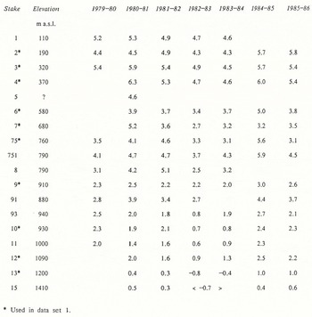
Summaries of the most recent glaciological and climatological statistics from Qamanârssûp sermia have been given by Reference BraithwaiteBraithwaite (1987). The data analysed here refer to annual values of net ablation measured at stakes on Qamanàrssûp sermia (Fig. 1) for varying periods within the 7 years 1979–80 to 1985–86. The data are summarized in Table I where a sign convention of “positive” ablation is used, in contradiction to “negative” ablation as recommended in Anonymous (1969), because it is more logical to do so. The data can be understood as annual balances with the sign reversed. With the exceptions of the 3 years 1982–83 and 1983–84, when the equilibrium-line altitude lay below stake 13 at 1200 m a.s.l., the stakes all lie in the ablation area.

Fig.1. Sketch map of Qamanârssûp sermia. West Greenland, showing locations of ablation stakes. The 1200 and 1500 m contour lines are approximate.
Stakes up to and including stake 8 (790 m a.s.l.) usually have little or no winter snow cover and their net ablation mainly reflects melting, of which about 80–90% occurs in the period June-August. At and above stake 9 (910 m a.s.l.), there is a fairly substantial winter snow cover which starts to melt in mid-May or early June but, for a variety of reasons, satisfactory measurements of winter accumulation have not been obtained for all years. The “751” stakes (actually three stakes placed within a few metres of each other) near to base camp were read almost every day during the summer, while other stakes were read more sporadically. The less accessible stakes, from stake 9 to 13, were often read only two or three times during the summer, while a final reading of stake 15 was totally missed in 1 year (1982–83) because of bad weather at the end of the season. The last stake readings of the summer were usually made as close as possible to the end of August and then the data were adjusted with the daily ablation readings from the “751” stakes so that annual values were calculated for a measurement year 1 September-31 August.
Although the data in Table I refer to repeated measurements on the same stakes, conditions at each stake are not constant. Stakes move with speeds up to 250 m a−1 in the middle of the glacier, while the main topographic features such as ice falls, crevasse zones, and smooth areas,appear to remain fixed. This means that each stake passes through a variety of local topography so the series at each stake is not homogeneous, but is sampled over trajectories of up to 1–2 km. However, this might have the effect of randomizing the smaller-scale effects of local topography so that the data reflect broader-scale factors like elevation, distance from the glacier margin, and large-scale topography.
Table.1. Annual net ablation at 19 stakes, qamanÂRSSÛp sermia, west greenland. units are m water a−1. The measurement year is 1 september- 31 august
The data are also affected by errors. For example, the error in annual ablation data is about ±0.23 m water a−1under the best conditions, i.e. the “751” stakes which are read almost daily, while errors at more distant stakes could be larger (Reference BraithwaiteBraithwaite, 1986). There are also some gross errors in the data in Table I and, as shown later, some of these can be identified by the inter-stake correlations.
The Problem
Ablation variations at different stakes tend to follow each other from year to year, e.g. ablation for 1982–83 was generally low for all stakes, while values for 1984–85 were high (Table I). This is illustrated by correlations between time series at the different stakes which are plotted in Figure 2 against elevation differences between the stakes concerned.
As might be expected, there are some high correlations between stakes but there are also disturbingly many low correlations, indicating that ablation variations at some stakes have little or no relation to variations at other stakes. For example, the average correlation coefficient in Figure 2 is only 0.61 (standard deviation ±0.30). Do these low correlations contradict the linear model applied by Reference BraithwaiteBraithwaite (1986) which implies that ablation at different stakes has the same time variations? The question is important because the validity of measuring mass balances at a few stakes over large areas, as done in Greenland, rests upon the approximate correctness of the linear model. The problem is approached here by developing a simple theory to relate inter-stake correlations to the assumptions of the linear model.

Fig.2. Correlations between annual net ablation at different stakes versus elevation differences between stakes. Sample sizes are from 4 to 7 years.
Theory
Linear model
Annual ablation on a glacier is assumed to vary from year to year and from place to place according to the simple relation:
where yit is the annual ablation at stake i in the year t, αi -varies with stake, ßt varies with year, and εit , varies with both year and stake. The variable ß t is the climate signal and εit is the random noise caused by measurement errors, variations in local topography, etc. Both ß 1 and εit are stationary random processes. The noise εit is uncorrelated with climate signal βt as well as being uncorrelated with noise at other stakes. It is an important hypothesis that βt , is the same for all stakes.
Equation (1) was first proposed by Reference LliboutryLliboutry (1974) for comparing balances at different stakes on a single glacier and has been used for that purpose by Reference KuhnKuhn (1984), Reference BraithwaiteBraithwaite (1986), and Reference Reynaud, Vallon and LetréguillyReynaud and others (1986). Reference ReynaudReynaud (1980) and Reference Reynaud, Vallon, Martin and LelréguillyReynaud and others (1984) have also used the model for inter-glacier comparisons.
Both βt and εit are defined so that their time averages are zero, i.e. that:

where N is the period of record in years. Time-averaging both sides of Equation (1) shows that α( is equal to the time average y i of the annual ablation at stake i:

The stake average of εit is also zero by asssumption. Stake-averaging both sides of Equation (1) gives:

The above is valid for a complete data set, i.e. for M stakes in N years. The calculation is more complicated for incomplete data, e.g. see Reference LliboutryLliboutry (1974) for a least-squares procedure. By definition, the time variance of yit is:

where Sy is the standard deviation of annual ablation which is assumed to be the same for all M stakes, i.e. ablation variations are assumed to be spatially homogeneous. Similarly, the variance of βt (mean value zero by assumption) is:

where SB is the standard deviation of climate signal βt which is assumed to be the same for all stakes. The standard deviation Sc of noise εit is defined in a similar way. By assumption, the climate signal βt and the noise εit are not correlated with each other which gives:
This states that the time variance of ablation is the sum of variances of the climate signal and of the noise.
The variables αi, βt, and εit are only defined in terms of a complete data set for M stakes and N years. This is a disadvantage because it pre-supposes that all data satisfy the assumptions of the linear model but this can be checked by inter-stake correlations.
Inter-stake correlations
By definition, the correlation between annual ablation values at stakes i and j, i.e. inter-stake correlation of ablation, is given by:

Substitution of Equation (1) into Equation (8), applying the definitions of the variances from Equations (5) and (6), and recalling that βt and εit are uncorrelated, gives:
where the factorś (SB/Sy)2 and (Sc/Sy)2 are the fractions of ablation variance accounted for by climate signal and noise, respectively. In the special case that i = j, both the correlations in the above equation are equal to unity so that Equation (9) becomes identical to Equation (7). For the more general case of i ≠ j, the correlation R(εit, εjt) is zero by assumption, so that:
which states that the inter-stake correlation of annual ablation is constant and equal to the variance ratio (SB/Sy)2, i.e. a small error in the linear model favours a high inter-stake correlation. According to Equation (10), the simple linear model in Equation (1) can be tested by calculating correlation coefficients between ablation values at different stakes and checking that they are roughly constant (and reasonably high).
Ablation-climate correlations
By an analogous process, the correlation between annual ablation yit and an arbitrary time series ft is given by:
The ratio (SB/Sy) is never greater than unity, which means that R(yit, ft) is less than or equal to R(βt, ft). This means that the effect of noise in ablation data is to reduce correlations between ablation at individual stakes and other time series, while the calculation of climate signal involves suppression of noise. An interesting special case arises with ft = βt so that R(yit,βt) = (SB/Sy) in this case, indicating that the climate signal βt is the time series that correlates best with measured ablation.
Non-stationary data
The treatment assumes that all time variations are stationary, i.e. ablation variations are measured in a constant climate. This is a reasonable assumption for the short series discussed here; it would be very difficult to demonstrate a statistically significant trend in the data. However, for longer glaciological series extending into a future greenhouse climate, non-stationary data will become important (as kindly pointed out by an anonymous referee). If there is a trend of rising ablation, αi will increase with length of series (because mean ablation will increase with time) and βt, for any particular series, will have a trend superimposed on random variations. The precise treatment for this case can be left until it is relevant but there are two possible approaches: (1) to detect and remove trend from the ablation data yit before applying the model; (2) to detect trend in the calculated climate signal βt after applying the model which would ensure calculation of a common trend for all stakes.
Results
For the present analyses, neither stakes close to the glacier edge nor stakes with incomplete series are used. There are only five stakes satisfying these conditions for 7 years (1979–80 to 1985–86), i.e. stakes 2, 3, 75, 9, and 10.The study is therefore restricted to only 6 years (1980–81 to 1985–86), for which complete data are available at ten “centre-line” stakes, i.e. the stakes 2, 3, 4, 6, 7, 75, 9, 10, 12, and 13 (marked with asterisks in Table I).
Inter-stake correlations
Correlation coefficients for 6 year ablation series at each of ten stakes are correlated with series at the other nine stakes. The resulting 90 correlation coefficients are summarized in the first column of Table II in the form of means and standard deviations of the nine correlations for each stake. The mean correlation is 0.64 with a quite large standard deviation. However, it is clear that two stakes (stakes 7 and 75) have mean correlations substantially below the average. Suspecting gross errors in the data, inspection of the original field books shows that the ablation value of 5.2 m water a−1 for stake 7 in 1980–81 cannot be supported. Eliminating stake 7 from the data set and repeating the calculations gives the results in Table II for data set 2. Although the mean correlation is increased, correlations for stake 75 are still well below the average. Eliminating stake 75 from the data set gives data set 3 with an increased mean correlation of 0.77 and a reduced standard deviation of ±0.13.
Inter-stake correlations for data set 3 have little correlation (R = 0.12 for a sample size of 28) with increasing elevation difference between stakes which agrees with Figure 2. However, inter-stake correlations have a moderate correlation (R = 0.61) with the mean elevation of the stake pair. The higher stakes in Table II, i.e. stakes 9–13, also have higher average inter-stake correlations than the lower stakes, i.e. stakes 2–6. The reason may be that the higher stakes are located in smoother areas than the lower stakes, so that effects of local topography are less.
Linear model
The standard deviations of climate signal and noise for the simple linear model in Equation (1) are given in Table III for the three data sets based on ten, nine, and eight stakes, respectively. The noise standard deviation Sc decreases from ±0.40 to only ±0.28 m water a−1 with elimination of data from stakes 7 and 75, while the standard deviation of the climate signal remains fairly constant at ±0.55 m water a−1. The variance ratio (SB/SV) thereby rises from 0.65 to 0.79, i.e. the climate signal accounts for almost four-fifths of the time variance of ablation after eliminating suspect data. This shows that the noise in the linear model is very sensitive to gross errors in the data. This is also illustrated by the frequency distributions in Figure 3 which show the noise values for the individual stakes and years.
Aside from illustrating the reduction of noise by eliminating suspect data, the results show close agreement between inter-stake correlations and variance ratios with coefficients of 0.97–0.98 compared with unity predicted by Equation (10). This shows that the climate signal ßt is nearly the same for all locations, in agreement with the simple linear model in Equation (1).
Table.2. Correlations of annual net ablation for each stake with every other stake

Table.3. Comparison of results of inter-stake correlations and the linear model


Fig.3. Frequency distributions for errors in the linear model for ten and eight stakes, respectively,

Fig.4. Stake-to-stake variations of annual net ablation. The mean refers to the 6 years 1980–81 to 1985–86; “Low” refers to 1982–83 and “High” refers to 1984–85.
The statistical results are supplemented by Figure 4, which shows the inter-stake variation of annual net ablation for the eight stakes in data set 3. The central trace refers to the 6 year mean values, while the “High” and “Low” traces refer to the two extreme years 1984–85 and 1982–83. There is a strong impression of parallelism, although the traces do not follow each other perfectly. This is a graphical expression of the combined effects of climate signal and noise.
Climate signal
The climate signal βt for the 6 years is summarized in Table IV for the three data sets. The three sets of values are surprisingly similar. For example, all three agree that the year 1982–83 had the lowest ablation and 1984–85 the highest ablation, while 1981–82 was close to normal. The climate signal is therefore not especially sensitive to gross errors in the data. The standard deviation Sb for data set 3 is ±0.55 m water a−1, which is in close agreement with the corresponding values from Nordbogletscher in Johan Dahl
Land, south Greenland (Reference Braithwaite and OlesenBraithwaite and Olesen, 1988), and from Glacier 1CG14033, West Greenland (Braithwaite and Thomsen, in press).
The climate signal only accounts for about 7% of the total ablation variations in data set 3, while noise accounts for 2% and the remaining 91% are caused by variations between stakes. Time variations of ablation are therefore much smaller than spatial variations in a widely dispersed stake network. This means that climate signal can only be identified if the same stakes are used in all years.
Ablation-climate relations
Correlations between annual net ablation ait and other series are shown in Table V. These are climate signal βt, ablation at the “751” stakes at*, and annual precipitation (September-August) and summer mean temperature (June-August) at the nearest permanent weather station Nuuk/Godthåb which is about 150 km west of Qamanârssûp sermia. The results for correlations involving ait in the top line of Table V refer to means and standard deviations of correlations for the eight stakes in data set 3. Other numbers refer to single correlations.
The climate signal should be better correlated than other series with measured ablation ait, and this is the case in Table V with a mean correlation of 0.89. The ratio (SB/Sy)identical value (the square root of 0.79 in Table III) in agreement with Equation (11). Correlations between ait and the other three series are lower than the corresponding correlations with βt by factors of 0.91, 0.88, and 0.89, respectively, which are in good agreement with the expected factor 0.89. This shows that glacier-climate correlations should be made with data for individual stakes.
The strong correlation (R = 0.85) between climate signal and summer temperature agrees with Reference Braithwaite and OlesenBraithwaite and Olesen (1985, 1989). The sensitivity of net ablation to change in summer temperature, i.e. slope of regression line, is 0.61 m water a−1 deg−1. The fairly strong negative correlation (R = −0.81) between climate signal and precipitation partly reflects the negative correlation between annual precipitation and summer temperature (R = −0.64) but also reflects the role of accumulation in inhibiting ablation as on Nordbogletscher (Braithwaite and Olesen, in press).
Annual ablation at the “751” stakes at* has fairly high correlations with both the measured ablation and climate signal. This justifies the inclusion in the field programme of such a measurement as an index of ablation in other parts of the glacier. In particular, ablation can be measured daily at the “751” stakes, while climate signal can only be determined on an annual basis.
Implications
Glaciers and climate
Time variations of ablation caused by climatic fluctuations, i.e. climate signal, can be obtained from sparse stake networks by using the linear model, while inter-stake correlations can be used to check the validity of the model. The linear model and inter-stake correlation method can also be applied to the simplified stake lay-outs discussed by Reference KoernerKoerner (1986), i.e. a line of stakes over a large elevation interval or a “stake farm” covering a small area of the glacier. Ablation variations can therefore be measured from year to year without the expense of sampling the whole glacier, although the same stakes should be used throughout the measuring period. For long ablation series, e.g. 20–30 years which is not yet the case in Greenland, it is inevitable that stakes will be lost or so greatly displaced by ice movement that the data will not be homogeneous. In these cases, overlapping 5–10 year sub-series of selected stakes could be established and “patched” together to make a longer homogeneous series.
Table.4. Climate signal for qamanÂrssÛp sermia extracted by the linear model. units are m water a−1

Table.5. Correlations between annual net ablation ait, climate signal βt , ablation at the “751” stakes at*, and annual precipitation pt, and summer mean temperature Tt in nuuk/godthÂb

The sparse stake-network concept should be extended to the whole Greenland ice sheet to develop a monitoring system for future climatic change. According to present results, such a system needs to detect trends of increasing ablation (about 0.61 m water a−1 deg−1 in the present case) against a background of year-to-year fluctuations (±0.55 m water a−1) and measurement errors (±0.28 m water a−1). There is no evidence yet of increasing ablation in Greenland due to the greenhouse effect, e.g. Reference Braithwaite and ThomsenBraithwaite and Thomsen (1989) suggest that ablation—climate conditions in the early 1980s are close to the average for the last century.
It is not certain that ablation variations under a future greenhouse climate will obey the linear model exactly. For example, the relation between ablation and degree days claimed by Reference Braithwaite, Olesen and OerlemansBraithwaite and Olesen (1989) suggests that a certain temperature change will change ablation in proportion to the already existing ablation, i.e. the ablation increase will be greatest at the margin and will fall with elevation. This question will be investigated further.
Glacier hydrology
According to results from Nordbogletscher in south Greenland (Reference Braithwaite and OlesenBraithwaite and Olsen, 1988), the annual runoff from a glacierized area varies as a linear combination of climate signal and annual precipitation, with the former becoming increasingly important for highly glacierized basins. The close similarity of results for Qamanârssûp sermia and Nordbogletscher is illustrated in Figure 5 which compares the climate signals for Nordbogletscher and Qamanârssûp sermia with annual precipitation variations for Narssarssuaq and Nuuk/Godthåb, the nearest permanent weather stations to the two glaciers. Aside from the near overlapping of the two precipitation traces, and of the two climate signals, the inverse relation between precipitation and climate signal is clear. This has important consequences for hydrology in that precipitation and ablation variations tend to offset each other so that run-off variations are smoothed in outlet streams from basins with a moderate amount of glacier cover (Reference Braithwaite and OlesenBraithwaite and Olesen, 1988).

Fig.5. Ablation signal for Qamanârssûp sermia and Nordbogletscher plotted together with annual precipitation in Narssarssuaq and Nuuk/Godlhåb. respectively.
Conclusions
Annual net ablation on Qamanârssûp varies from stake to stake and from year to year. Positive correlation coefficients between ablation data at different stakes are caused by the climate signal which is common to all the stakes. Low, and even negative, inter-stake correlations are caused by gross errors in the data which can be detected by comparing inter-stake correlation coefficients for the different stakes. Elimination of such errors reduces noise variations while climate signal is less affected. The climate signal for Qamanârssûp sermia is strongly correlated with both summer temperature and annual precipitation. Present results therefore confirm an earlier conclusion (Briathwaite, 1986) that even sparse stake networks, as used in Greenland, give useful glacier-climate information.
Acknowledgements
This paper is published by permission of the Geological Survey of Greenland. We thank the many assistants who helped to collect data at Qamanârssûp sermia, especially those who came for at least two seasons: J. Andsbjerg, C. Bøggild, B. Christiansen, I. Eiríksdóttir, and A. Engraf (all from Copenhagen University), and J.-O. Andreasen and O. Bendixen (both from Aarhus University). An anonymous referee made valuable comments. G.F. Hansen prepared the drawings.


