

1. INTRODUCTION
Prokaryotes, which include the Bacterial and Archaeal domains, are the predominant organisms on Earth in terms of numbers and biomass (Whitman and others, Reference Whitman, Coleman and Wiebe1998). They are also the most physiologically diverse and structurally simple group of organisms (e.g. Meyer, Reference Meyer1993; White, Reference White2007), appearing on Earth ~3.5 Ga BP (Rasmussen, Reference Rasmussen2000; Noffke and others, Reference Noffke, Eriksson, Hazen and Simpson2006; Javaux and others, Reference Javaux, Marshall and Bekker2010). Prokaryotes are drivers of key ecosystem functions such as nutrient cycling, degradation and mineralization of organic carbon and the regulation of global gas levels, all of which play an important role in the climate system (Finlay and others, Reference Finlay, Maberly and Cooper1997; Field, Reference Field1998; de Groot and others, Reference de Groot, Wilson and Boumans2002; Falkowski and others, Reference Falkowski, Fenchel and Delong2008; Madsen, Reference Madsen2011). They have driven important changes in atmospheric composition such as the Great Oxidation Event (~2.45 Ga), a consequence of the evolution of oxygenic photosynthesis (Kasting and Siefert, Reference Kasting and Siefert2002; Kopp and others, Reference Kopp, Kirschvink, Hilburn and Nash2005; Kump, Reference Kump2008).
Despite the critical role of microorganisms during the evolution of the Earth system, they are not explicitly part of predictive climate models (Schimel, Reference Schimel and Schulze2001; Singh and others, Reference Singh, Bardgett, Smith and Reay2010). Their absence in climate models is the result of an incomplete understanding of microbial community responses to long-term climatic and environmental processes and therefore, their potential to influence climatic feedbacks (Schimel, Reference Schimel and Schulze2001; Singh and others, Reference Singh, Bardgett, Smith and Reay2010). Experimental and observational studies have indicated that microbial communities (abundance, composition and diversity) can significantly respond to and impact ecosystem-level processes at short-time scales (Castro and others, Reference Castro, Classen, Austin, Norby and Schadt2010; Yergeau and others, Reference Yergeau2012; Singh and others, Reference Singh2014; Park and others, Reference Park, Kug, Bader, Rolph and Kwon2015). In contrast, long-term perspectives obtained from paleorecords can present historical views old enough for a range of climate and ecosystem variability to occur (Gorham and others, Reference Gorham, Brush, Graumlich, Rosenzweig and Johnson2001; Jackson and Erwin, Reference Jackson and Erwin2006; Willis and Birks, Reference Willis and Birks2006; Willis and others, Reference Willis, Bailey, Bhagwat and Birks2010). An important archive of past climatic events is preserved in ice sheets. Although climatic and environmental changes have been well recorded and reconstructed from physical, chemical and isotopic records from polar ice cores (e.g., Dansgaard and others, Reference Dansgaard1993; Lüthi and others, Reference Lüthi2008; Wolff and others, Reference Wolff2010), no comprehensive prokaryotic record from ice cores exists owing to a lack of clean and time efficient methods to measure these microorganisms.
Total prokaryotic cell concentrations have been shown to be present in the atmosphere at levels ranging between 103 and 109 cells m−3 (e.g., Griffin and others, Reference Griffin2003; Griffin, Reference Griffin2007; Burrows and others, Reference Burrows, Elbert, Lawrence and Poschl2009a, Reference Burrowsb; Perfumo and Marchant, Reference Perfumo and Marchant2010; Hara and Zhang, Reference Hara and Zhang2012). These cells can be incorporated in glacial ice through dry and wet deposition at the surface of the ice. After deposition, the microorganisms are encased and incorporated into glacier ice (Barrie, Reference Barrie1985; Davidson and others, Reference Davidson, Bergin, Kuhns, Wolff and Bales1996; Priscu and others, Reference Priscu, Christner, Foreman and Royston-Bishop2007; Xiang and others, Reference Xiang, Shang, Chen and Yao2009). There, they can persist over extended periods of time due to the deeply frozen conditions within the Antarctic ice sheet (Priscu and Christner, Reference Priscu and Christner2004). Prokaryotes have been identified, cultured and quantified from discrete ice-core samples using both culture-dependent (e.g. Abyzov and others, Reference Abyzov, Mitskevich and Poglazova1998; Christner and others, Reference Christner2000; Miteva and others, Reference Miteva, Sheridan and Brenchley2004) and culture-independent methods (e.g. Sheridan and others, Reference Sheridan, Miteva and Brenchley2003; Priscu and others, Reference Priscu, Christner, Foreman and Royston-Bishop2007; Miteva and others, Reference Miteva, Teacher, Sowers and Brenchley2009). To date, studies of prokaryotes have been limited to selected sections of ice cores and lack the high-temporal resolution to record their history through various climate scenarios.
Here, we describe a protocol using an ice-core melting system in combination with flow cytometry (FCM) of DNA-stained cells. To demonstrate its potential as a method to resolve non-photosynthetic prokaryotic concentrations in paleoclimatic studies of ice cores, we applied this method to a section of the West Antarctic Ice Sheet (WAIS) Divide (WD) ice core (2100–2480 m). We show that the use of FCM with a specific DNA stain allows the accurate and precise measurement of prokaryotic concentrations in ice cores, providing a millennial prokaryotic record.
2. MATERIALS AND METHODS
2.1. Samples
2.1.1. Core samples
Two sets of ice-core samples collected from the WD site were used in this study. The first sample set represents core sections 74, 85, 94 and 105 m below the surface collected in December 2005 (WDC05Q core; Banta and others, Reference Banta, McConnell, Frey, Bales and Taylor2008). Following decontamination according to Christner and others (Reference Christner, Mikucki, Foreman, Denson and Priscu2005), the samples were melted at 4°C and combined to obtain a total melt volume of 280 mL. The second set corresponds to discrete meltwater samples from the deep WD ice core (WDC06A) retrieved between 2009 and 2011. Discrete liquid samples (1–8 mL) were obtained using a continuous ice-core melting system at the Desert Research Institute (McConnell and others, Reference McConnell, Lamorey, Lambert and Taylor2002). The depth range for the WDC06A analyzed section was 2100–2480 m. These melted samples have a depth resolution from 25.4 to 98.7 cm (2.12–33.0 a) with a depth resolution average of 65.5 cm, resulting in a mean time resolution of 12.1 a.
2.1.2. Bacterial cultures
Two Antarctic bacterial isolates from the Cotton Glacier (Dieser and others, Reference Dieser, Greenwood and Foreman2010) and Lake Vostok accretion ice (Priscu and others, Reference Priscu1999; Christner and others, Reference Christner2006) were used as test organisms during method development. The cultures were grown in 500 mL bottles and continuously shaken at 150 rpm in a 7°C temperature-controlled incubator. They were fixed with 0.2 µm filtered formalin (2% final concentration) once stationary phase growth was reached. The fixed bacterial cultures were immediately concentrated by centrifugation at 4600 g for 10 min in a 50 mL centrifuge tube at 10°C and washed four times with Milli-Q water. The cultures were re-suspended in Milli-Q water to 600 mL at a concentration of 107 cells mL−1 and stored at 4°C until use.
2.1.3. Glacier sediments
Heat-sterilized control sediments from Robertson Glacier (Canada) were combusted at 450°C for 3 h to eliminate organic matter. The sediments, composed primarily of calcite, dolomite, quartz, k-feldspar and muscovite, were then screen fractionated into <63 and 63–125 µm size classes for experimental use. Following this treatment, sediments were mixed in varying configurations with the bacterial cultures to assess the degree to which they interfere with the flow cytometric assay.
2.2. Ice-core melter
The well-established ice-core analytical system located at Desert Research Institute includes an array of mass spectrometers, fluorometers, spectrophotometers and other instruments for continuous determination of ~35 elements, chemical species, and isotopes (adapted from McConnell and others, Reference McConnell, Lamorey, Lambert and Taylor2002). The melting system resides in a −20°C clean cold room, with many measurements conducted in near-real-time in an adjacent class-100 clean room (ISO 5). To avoid contamination from the external part of the core, the samples for microbiological characterization were taken from the 1.3 cm × 1.3 cm center ring (total area = 1.69 cm2) of the three-ring melter plate. This region represents the inner-most ~10% of the sample cross section. The meltwater from the inner ring was pumped from the melter head through polytetrafluoroethylene (PTFE) tubing (0.76 mm i.d.). The meltwater was captured in 8 mL amber borosilicate glass vials with PTFE liner caps previously acid-washed (10% HCl) and combusted (450°C for 4 h). The sample collection system was automated using a Gilson temperature controlled (4°C) fraction collector so that known volumes of sample were dispensed into the vials using a large needle to penetrate the septa at a melting rate of ~4 cm min−1, (i.e. the vials were never opened once combusted). To minimize potential contamination, deionized water (after two stages of cleaning: reverse osmosis and deionization using mixed-bed resin filters, further cleaned in the ice-core laboratory using an Elga Pure Laboratory Ultra polishing unit) was used routinely to rinse and irrigate the melter head between ice sections. The discrete melted glacial samples were fixed with 0.2 µm filtered formalin (2% final concentration) and stored at 4°C until analysis. Additional longitudinal ice sections from the same core taken from parallel depths were used to repeat measurements. The replicate sections were melted between 1 and 60 d after the original sections, to demonstrate the reproducibility of prokaryotic density sample acquisition by the ice-core melter system. Each of those replicate sections had a cross-sectional area of ~3 cm × 3 cm and they represented ~10% of our target ice-core section (2100–2480 m).
2.3. Flow cytometer
FCM measurements were made using a PhytoCyt flow cytometer (Turner Designs), which was developed in partnership with Accuri Cytometers (equivalent to the Accuri C6 BD model). This flow cytometer analyzes up to six simultaneous parameters, using two scatter measurements: 0° light forward-scatter (FSC, ±15°) and 90° light side-scatter (SSC, ±15°), and four fluorescence parameters: (1) green fluorescence (FL1; 530 ± 15 nm; excitation at 488 nm), (2) yellow/orange fluorescence (FL2; 585 ± 20 nm; excitation at 488 nm), (3) red fluorescence-blue laser excitation (FL3; 670 LP nm; excitation 488 (blue laser)), and (4) red fluorescence-red laser excitation (675 ± 12.5 nm; excitation 640 nm (red laser)). The PhytoCyt is equipped with a solid-state laser (20 mW; 488 nm; blue laser) and a diode laser (30 mW; 640 nm; red laser). The detectors consist of a photodiode for the FSC from the blue laser, and a photomultiplier (PTM) for the SSC and the fluorescence emissions. Sample acquisition (24 bits and 7 decades digitization) and data analyses were performed using CFlow® software. This software allows the FCM parameters to be obtained as area (A), height (H) or width (W). All parameters were recorded on a seven-decade logarithmic scale for FCM controls and samples.
The instrument was installed in a clean bench with UV light (Labconco). Standard validation beads (Spherotech 8- and 6-Peaks Validation Beads) were analyzed daily to validate the system's fluidic performance and the instrument's level of sensitivity in detecting events. Milli-Q water blanks were measured before samples, and three back-flushes were performed between samples to prevent carry-over between them.
2.4. Nucleic acid stains
The nucleic acid stains tested in this study were SYTOX-green® and SYBR-green-I® (Molecular Probes Inc). SYTOX-green, the stain ultimately chosen, is an asymmetrically cationic triple-charged cyanine dye of 600 Dalton (Molecular Probes; Bojsen and others, Reference Bojsen, Torbensen, Larsen, Folkesson and Regenberg2013). SYTOX-green cannot cross the membranes of live cells and can only enter cells with compromised membranes (Roth and others, Reference Roth1997; Lebaron and others, Reference Lebaron, Catala, Parthuisot and Oce1998a; Jones and Singer, Reference Jones and Singer2001). It has a fluorescence quantum yield of 0.53 when bound to DNA (i.e. number of photons emitted/number of photons absorbed), with an excitation maxima at 480–505 nm, and emission maxima of 523 nm (Roth and others, Reference Roth1997; Mortimer and others, Reference Mortimer, Mason and Gant2000; Jones and Singer, Reference Jones and Singer2001; Burnett and Beuchat, Reference Burnett and Beuchat2002). SYBR-green-I is a monomeric unsymmetrical cyanine dye that is capable of penetrating intact cell membranes. SYBR-green-I has been broadly used to quantify microorganisms in aquatic systems (Marie and others, Reference Marie, Partensky, Vaulot and Brussaard1999; Gasol and del Giorgio, Reference Gasol and del Giorgio2000) and has a fluorescence quantum yield of 0.80 for DNA and 0.40 for RNA; it is maximally excited at 494–497 nm, and has an emission maximum at 521 nm (Molecular Probes; Lebaron and others, Reference Lebaron, Parthuisot, Catala and Oce1998b). Both stains were diluted in 0.2 µm filtered 1× TBE (5.4 g Tris, 2.75 g Boric acid, 0.5 m EDTA, pH 8.0) before use.
2.5. Epifluorescence microscopy (EFM)
Samples for EFM were prepared inside a laminar-flow hood (Purifier horizontal clean bench, Labconco). The samples were stained for 20 min at a final concentration of 2.5 µm for SYTOX-green and 1× for SYBR-green-I (Marie and others, Reference Marie, Partensky, Vaulot and Brussaard1999). Following staining, samples were filter concentrated onto Millipore Isopore™ Polycarbonate membrane filters (GTBP1300, 0.22 µm pore size, 13 mm diameter, black) using Swinnex® 13 filter holders and sterile syringes. Each filter was mounted on a glass slide with a drop of 0.2 µm filtered antifade solution (1:1 glycerol, PBS and 0.1% p-phenylenediamine) before covering the filter with a 20 mm square coverslip. All prokaryotic cell counts were performed at 1000× with a Nikon Eclipse 80i epifluorescence microscope equipped with a Metal Halide lamp (X-Cite® 120W), a 450–490 excitation filter (B-2A), a 515 barrier filter and a digital CCD Camera (Retiga 2000R Color Cooled). The total prokaryotic cell number was estimated on each filter by counting at least 500 cells per filter or up to 60 microscope fields, whichever occurred first. Controls consisted of filtered Milli-Q water (same volume as for samples) and were counted along with the samples on a daily basis. Because low cell concentrations were expected and only low sample volumes were available (~1–8 mL), the Swinnex filter holders were modified to reduce the filtration area to 2.5 mm diameter when required. The small filtration area permitted the effective filter surface and counting effort to decrease when samples have low cell concentrations. A total of 110 WD samples were analyzed in parallel by FCM and EFM.
2.6. Field emission scanning electron microscopy (FE-SEM)
Equal volumes of 45 WD samples representing the Last Glacial Maximum (LGM) were combined to yield a 15 mL composite for this period (23 420–19 978 a before 1950 CE) and equal volumes of 58 discrete samples representing Termination I were combined to yield a 30 mL composite for this period (12 343–11 726 a before 1950 CE). These composite samples were fixed for 20 h in 5% (v/v) glutaraldehyde. Cells were then filter concentrated onto Isopore™ filters (GTBP01300, 0.22 µm pore size, 13 mm diameter, Millipore) with sterile Swinnex® filter holders (13 mm diameter, Millipore). The fixed cells were dehydrated by sequential passage through an ethanol gradient ranging from 10 to 100% ethanol (in increments of 10%; 10 m at each concentration), dried in a Tousimis Samdri-795 critical point dryer, coated with Iridium using an Emitech K575X coater and visualized using a Zeiss Supra 55VP FE-SEM.
2.7. Protocol development
Different protocols were investigated to select the most accurate and precise method for the WD ice-core samples following the Minimal Information in FCM Experiments protocols (MIFlowCyt), outlined by Lee and others (Reference Lee2008). Data from FCM are often subjective and results can be ambiguous due to the lack of guidelines, controls and specific gating strategies in many publications (Lee and others, Reference Lee2008; Müller and Tárnok, Reference Müller and Tárnok2008; Nebe-von-Caron, Reference Nebe-von-Caron2009). Because of their small size, prokaryotic cells are at the limits of the detection sensitivity of most flow cytometers and require extra care to avoid and minimize interference factors (Müller and Tárnok, Reference Müller and Tárnok2008; Nebe-von-Caron, Reference Nebe-von-Caron2009). For these reasons, and to provide the reader with a detailed protocol, FCM controls, optimizations, gating strategy and instrument setups are addressed in depth in this paper. All statistical tests were conducted using R-programming language (version 2.15.0 by R Foundation for Statistical Computing; R Development Core Team, 2012).
2.7.1. Clean conditions
A clean environment is required for unequivocal results, particularly when sample volume and cell density are low. These requirements are necessary not only to prevent contamination and increase the accuracy of cell quantification, but also to reduce the background noise on the FCM system, which improves sensitivity of the signal (Steen, Reference Steen1992, Reference Steen2000). We tested the efficacy of our clean methods using sterile Milli-Q water for FCM analysis and handled all samples in a laminar flow environmental chamber with UV light, using sterile materials (e.g., pipet tips, gloves, forceps) and appropriate sterile clothing, including face mask and hair cover. Events from 300 µL of Milli-Q water were acquired by FCM using these conditions and compared with samples processed on a laboratory bench with no sterile protocols. Five replicates were included for each scenario. The FCM data were analyzed using a t-test.
2.7.2. Instrument threshold level
The instrument threshold allows the reduction of electronic noise and background signals inherent to samples (Gasol and del Giorgio, Reference Gasol and del Giorgio2000; Shapiro, Reference Shapiro2003) at the expense of instrument sensitivity. The threshold is the lowest signal of relative intensity units (RIU) at which an event can be recorded, and each channel has an inherent (intrinsic) noise floor in all flow cytometers. The detection of the noise floor was recorded under clean conditions with pure water samples (Milli-Q water), setting the threshold to its lowest value in the green fluorescence channel and choosing the appropriate boundary in trial Milli-Q samples by visual inspection.
2.7.3. Establishing FCM controls
Controls allow objective recognition of DNA stained prokaryotic cells through their visual discrimination of fluorescence output (Lee and others, Reference Lee2008). Background signals that are inherent to samples and above the instrument threshold unavoidably occur. They have been reported in the literature and described as: non-specific stained particles, non-target cells, debris and/or unbound DNA stain (Klauth and others, Reference Klauth, Wilhelm, Klumpp, Poschen and Groeneweg2004; Müller and Nebe-von-Caron, Reference Müller and Nebe-von-Caron2010). The limits of background noise were determined using three FCM controls: (1) blank control – to ensure proper clean conditions were followed, (2) background control – to detect signals produced by stained particles smaller than prokaryotic cells (<0.22 µm), cellular debris and unbound stain (background controls are 0.22 µm filtered samples), and (3) negative control – to identify the unstained events (negative events) and autofluorescent events in unstained samples.
2.7.4. Selection of nucleic acid stain
Ice-core samples often contain high concentrations of prokaryotic sized abiotic (dust) particles (e.g. Fischer and others, Reference Fischer, Siggaard-Andersen, Ruth, Röthlisberger and Wolff2007). These abiotic particles can adsorb certain nucleic acid dyes and can also autofluorescence when exposed to low wavelength excitation light. These conditions can lead to: (1) false positive events in the prokaryotic cell size range, (2) a decrease of dye available to the target-cells, and (3) an increase in background noise (Klauth and others, Reference Klauth, Wilhelm, Klumpp, Poschen and Groeneweg2004; Müller and Nebe-von-Caron, Reference Müller and Nebe-von-Caron2010). To address these issues, an experiment was designed to determine which nucleic acid dye, SYTOX-green or SYBR-green-I, provides the most accurate cell counts in the presence of glacial sediments. These dyes were chosen because they have been used routinely to enumerate aquatic and soil bacteria by FCM.
Samples of bacterial cultures were serially diluted with Milli-Q water from x105 to x102 cells mL−1 (four different bacterial concentrations, three replicates each) followed by the addition of 0.2 mg of <63 µm glacial sediments to 1.9 mL samples to obtain a final concentration ~x104 sediment particles mL−1 and a final sample volume of ~2 mL. These samples were then stained for 20 min at 20°C in the dark followed by FCM analysis. The final stain concentrations used were 0.5 µm for SYTOX-green (Molecular Probes) and 1× for SYBR-green-I (Marie and others, Reference Marie, Partensky, Jacquet and Vaulot1997; Marie, 1999; stock concentration: 10 000×). Log/log linear regression between expected and observed cell densities from the FCM was compared with a 1:1 log/log linear relationship, which had an intercept (β 0) equal to 0 and a slope parameter (β 1) equal to 1.
2.7.5. Optimization of the stain concentration
Results from previous experiments showed that SYTOX-green revealed insignificant interference from glacial sediment, hence, optimization of stain concentration focused on this dye only. The recommended SYTOX-green concentration for bacteria ranges from 5 to 1 µm (Molecular Probes). We tested final concentrations: 1, 0.5, 0.25, 0.1, 0.05, 0.025 and 0.01 µm. SYTOX-green stocks (5 mm solution in DMSO) were diluted with 0.2 µm filtered 1× TBE (5.4 g Tris, 2.75 g Boric acid, 0.5 m EDTA, pH 8.0) and stored at 4°C in the dark before use. The final stain concentrations were tested on 1 mL samples of bacterial culture (1.3 × 10⁵ cells mL−1). The samples were stained with SYTOX-green, vortexed, incubated for 20 min in a sterile BD Falcon tube (12mm × 75 mm) at 20°C (room temperature) in the dark, and analyzed immediately by FCM.
2.7.6. Optimization of the fluidic settings in WD ice-core samples
The fluidic settings were performed on actual WD ice-core samples because these settings could modify cell detection and background noise (Gasol and del Giorgio, Reference Gasol and del Giorgio2000; Shapiro, Reference Shapiro2003). The flow rate that is used to enumerate prokaryotic cells by FCM is between 5 and 50 µL min−1 (Gasol and del Giorgio, Reference Gasol and del Giorgio2000). Low flow rates are typically used for dense prokaryotic cell samples to ensure there are no coincident particle counts; higher flow rates can be used for low density samples. Prokaryotic cells have been found in Antarctic ice-core samples at densities varying from ~1 up to 105 cells mL−1 (Christner and others, Reference Christner2006; Priscu and others, Reference Priscu, Christner, Foreman and Royston-Bishop2007; Segawa and others, Reference Segawa, Ushida, Narita, Kanda and Kohshima2010); hence it was imperative that an appropriate flow rate was chosen for the samples being processed.
In addition to the determination of a proper flow rate, we had to ensure that our sample prefiltration (to eliminate large particles that could clog the fluidics system) did not interfere with actual prokaryotic enumeration and background noise. We developed a single experimental design to determine both the effects of flow rate and pre-filtration on prokaryotic density (cells mL−1) and background noise events (events mL−1). The experiment was completely randomized with two fixed factors, flow rate and pre-filtration, each one with three treatments. For the flow rate factor, the treatments were: 14, 32 and 50 µL min−1. For the pre-filtration factor, the treatments were: no-pre-filtration, 30 µm pre-filtration and 100 µm pre-filtration. Each combination (9) had three replicates (3 × 9). The response variables were (1) prokaryotic density and (2) background noise events. A sample volume of 50 µL was analyzed for each of the 27 samples.
2.7.7. Validation of the measurement technique
All the samples used to validate the method were pre-filtered using a 30 µm mesh sterile BD Falcon Tube with Cell Strainer Cap and stained for 20 min in the dark at room temperature (~20°C) with SYTOX-green (final concentration of 0.05 µm). We determined FCM detection limits, the minimum cell concentration level at which the cell counts can be reliably detected, by comparing the observed versus expected cell densities of WD ice-core samples and bacterial cultures with added sediment. The samples were serially diluted with Milli-Q water to yield final cell concentrations ranging from 106 to 100 cells mL−1. A constant volume of 1600 µL was analyzed at a flow rate of 50 µL min−1 for each sample by FCM.
The relative precision of our method was computed as the coefficient of variation ( $\widehat{{{\rm CV}}} = ({\rm SD}/\bar X) \times 100$
); CV is the best precision estimator to describe variation that is proportional to the mean (Shapiro, Reference Shapiro2003; Bolker, Reference Bolker2008). By their nature, FCM counts should follow a Poisson sample distribution, a discrete distribution that describes count processes well. A characteristic of the Poisson distribution is that the variance is equal to its mean (σ
2 = μ). In other words, the variance depends on the number of counts. Therefore, the Poisson distribution becomes more regular as the expected number of counts increases (Shapiro, Reference Shapiro2003; Bolker, Reference Bolker2008); hence, the larger the number of cells counted by FCM, the greater the relative precision. The CV was calculated at different cell concentration factors in WD ice-core samples. A total of 23 random WD ice-core samples were analyzed with 2–4 replicates (replication depended on sample availability).
$\widehat{{{\rm CV}}} = ({\rm SD}/\bar X) \times 100$
); CV is the best precision estimator to describe variation that is proportional to the mean (Shapiro, Reference Shapiro2003; Bolker, Reference Bolker2008). By their nature, FCM counts should follow a Poisson sample distribution, a discrete distribution that describes count processes well. A characteristic of the Poisson distribution is that the variance is equal to its mean (σ
2 = μ). In other words, the variance depends on the number of counts. Therefore, the Poisson distribution becomes more regular as the expected number of counts increases (Shapiro, Reference Shapiro2003; Bolker, Reference Bolker2008); hence, the larger the number of cells counted by FCM, the greater the relative precision. The CV was calculated at different cell concentration factors in WD ice-core samples. A total of 23 random WD ice-core samples were analyzed with 2–4 replicates (replication depended on sample availability).
Accuracy was obtained using a log/log serial dilution curve to ensure that there was a log/log linear correlation between observed and expected bacterial densities over a range of cell concentrations. WD ice-core samples and bacterial cultures (with glacial sediments) were serially diluted by Milli-Q water from x105 to x102 cells mL−1 and three replicates were analyzed at each concentration by FCM. Accuracy was assessed by comparing the slope and intercept values of the 1:1 log/log regression with the log/log linear relationship between the observed and expected cell densities. The method was considered accurate if the 95% confidence intervals (CI) for both estimates, slope and intercept, includes the values of the 1:1 log/log linear regression (β 0 = 0; β 1 = 1).
2.7.8. Gating strategy
An important principle of FCM data analysis is to visualize the cells of interest while eliminating results from unwanted particles (non-target particles), in this case: cellular and abiotic debris, sediment particles and autofluorescent cells and particles (Shapiro, Reference Shapiro2003; Lee and others, Reference Lee2008). Six gates were set to obtain target-cell (non-photosynthetic prokaryotes) counts from WD ice-core samples. The final gating strategy was validated and described here, in the result section, using WD samples from depths ranging between 1307 and 2709 m.
3. RESULTS
3.1. Clean conditions and instrument threshold
There was significant evidence of an increase of background noise when the clean protocol was not used (one sided p-value < 0.05 from a two-sample t-test; Fig. 1c) indicating that the flow cytometer must be operated in a particle free environment and protective clothing must be worn.

Fig. 1. Cytograms showing results of forward-scatter-A and total particle counts versus green fluorescence-H (H = height) used to set instrument thresholds. (a1, a2): The equipment noise from an unstained Milli-Q water sample (blank); red lines were drawn to show the boundaries of equipment noise. (b1, b2): Unstained Milli-Q water sample (blank) after setting instrument threshold level at 750 RIU in FL1-H (green-fluorescence). (c1, c2): Unstained Milli-Q water sample with instrument threshold level set but without the use of clean protocols.
The instrument threshold was set on the same primary parameter (trigger signal) used to discriminate prokaryotic cells. This threshold was set on the green fluorescence channel (the FL1 detector) because SYTOX-green and SYBR-green-I have their maximum wavelength emission at 524 and 521 nm, respectively. The inherent noise floor for the green fluorescence channel was visualized by analyzing Milli-Q water with no stain and adjusting the threshold to its lowest value (10 RIU) in this FCM; Fig. 1a). The noise floor was subtracted by setting the threshold above the electronic noise in the green fluorescence channel. On our instrument, this resulted in threshold values of 750 RIU in the green fluorescence channel (vertical red line drawn on count versus green fluorescence plot; Fig. 1). Figure 1b shows the acquisition of events in a Milli-Q water sample after applying the instrument threshold at clean conditions where no events are recorded. It should be noted that the background noise is not all electronic and can increase significantly if clean protocols are not followed (Fig. 1c).
3.2. Establishing FCM controls
Three controls were established in this study (Fig. 2): (1) Milli-Q water blank controls, (2) background control consisting of sample filtered through a 0.22 µm pore size sterile filter followed by SYTOX-green staining, and (3) a negative control consisting of an unstained sample, which allows identification of autofluorescent particles and abiotic events. The background and negative controls provide information to set the boundaries of gate 1 (P1) where the expected positive events should fall (Fig. 2). This set of controls permits the recognition of DNA stained prokaryotic cells through their visual discrimination and the development of a protocol based on the outlined requirements in Minimal Information in FCM Experiments protocols (MIFlowCyt; Lee and others, Reference Lee2008).

Fig. 2. Cytograms on green fluorescence-H versus forward scatter-A density-plots of a WD sample. (a) Blank control = unstained Milli-Q water sample. (b) Background control = stained 0.2 µm filtered WD sample. (c) Negative control = unstained WD sample. Gate 1 (P1; red polygon) is used to keep outside background noise and negative events inherent to samples and is defined using these controls. Positive DNA stained events should fall in P1.
3.3. Selection of the nucleic acid stain
Quantitative results from the experiment to assess which stain, SYTOX-green or SYBR-green-I, accurately enumerate bacterial cells in the presence of sediments showed that: (1) SYTOX-green stained samples counted using gate 1 (P1) revealed similar counts with and without the addition of sediments (Fig. 3a) and (2) when SYBR-green-I was used to stain cells in the presence of sediments, the cell density decreased by factors of 28.3, 33.3 and 13.1 at tested prokaryotic densities of 103, 104, 105, respectively; no cells were counted at the expected cell density of 102 (Fig. 3b).

Fig. 3. Bacterial density in the presence of sediments for samples stained with SYTOX-green (panel a) and SYBR-green-I (panel b) in samples diluted with Milli-Q water. Gray bars correspond to bacterial density quantified for each stain in the presence of sediments; black bars correspond to the expected bacterial density. Inserts show a 1:1 log/log linear regression (red line) and actual observations (dots).
Statistical analysis, log/log linear regressions and CI, were used to assess the enumeration accuracy by both stains in the presence of sediments. We estimated the log/log linear regression between expected bacterial density (sample without sediments) and observed bacterial density (sample with sediments). We then compared the estimated log/log linear regressions with the parameters of the 1:1 log/log linear relationship. The parameters for the 1:1 log/log linear regression are an intercept (β 0) of 0 and a slope (β 1) of 1. We expected those values to be included in the 95% CI of the estimated log/log linear regressions. The estimated log/log linear regressions for the observed versus expected bacterial density were:
 $$\eqalign{{\widehat{{\log (y)}}_{{\rm SYTOX\; green}}} & = - 0.16 + 1.02\; \log (x);\; \cr \quad SE({{\hat \beta} _0}) &= 0.19\;{\rm SE}({{\hat \beta} _1}) = 0.02;\;{R^{\rm 2}} = 0.{\rm 99}} $$
 $$\eqalign{{\widehat{{\log (y)}}_{{\rm SYBR\; green\; I}}} & = - 7.91 + 1.43\log (x);\; \cr \quad {\rm SE}({{\hat \beta} _0}) &= 0.73\;{\rm SE}({{\hat \beta} _1}) = 0.07;\;{R^{\rm 2}} = 0.{\rm 97}} $$
Here, only the estimated 95% CI of SYTOX-green log/log linear regression included the values for the 1:1 log/log linear relationship $({\hat \beta _0} = [( - 0.58) - (0.25)];{\rm \;} {\hat \beta _1} = [(0.97) - (1.07)]$
). In contrast, the SYBR-green-I regression did not include the values of the 1:1 log/log regression in the 95% CI of the intercept and slope
$({\hat \beta _0} = [( - 0.58) - (0.25)];{\rm \;} {\hat \beta _1} = [(0.97) - (1.07)]$
). In contrast, the SYBR-green-I regression did not include the values of the 1:1 log/log regression in the 95% CI of the intercept and slope $({\hat \beta _0} = [( - 9.55) - ( - 6.27)];\ {\hat \beta _1} =$ $[(1.26) - ({\rm \;} 1.60)])$
. These results indicate that SYTOX-green accurately stains bacteria in the presence of glacial sediments, and SYBR-green-I showed non-specific staining for sediments. In addition, our microscopic inspection of samples showed that sediment particles and debris were not stained by SYTOX-green, whereas SYBR-green-I stained sediment particles and debris, which agrees with the results of other studies (Wobus and others, Reference Wobus2003; Klauth and others, Reference Klauth, Wilhelm, Klumpp, Poschen and Groeneweg2004; Morono and others, Reference Morono, Terada, Kallmeyer and Inagaki2013).
$[(1.26) - ({\rm \;} 1.60)])$
. These results indicate that SYTOX-green accurately stains bacteria in the presence of glacial sediments, and SYBR-green-I showed non-specific staining for sediments. In addition, our microscopic inspection of samples showed that sediment particles and debris were not stained by SYTOX-green, whereas SYBR-green-I stained sediment particles and debris, which agrees with the results of other studies (Wobus and others, Reference Wobus2003; Klauth and others, Reference Klauth, Wilhelm, Klumpp, Poschen and Groeneweg2004; Morono and others, Reference Morono, Terada, Kallmeyer and Inagaki2013).
3.4. Stain concentration
Seven SYTOX-green concentrations (1, 0.5, 0.25, 0.1, 0.05, 0.025 and 0.01 µm) were tested using WD ice-core samples to determine the optimal stain concentration. The stain concentrations that presented the highest mean and median gate 1 (P1) intensities of green fluorescence were 0.1 and 0.05 µm (Table 1). Although both of these concentrations produced high fluorescence yields and broad spectral difference between negative and positive events, the 0.05 µm treatment produced counts closer to the actual cell numbers (1.3 × 10⁵ cells mL−1) present in the samples, which was determined by direct microscopic counting. Results from these experiments led us to select 0.05 µm stain concentration for prokaryotic cell enumeration in the analyzed ice cores.
Table 1. Optimization of stain concentration

Mean and median fluorescence (RIU, relative intensity units) of P1 gate (prokaryotic events) in a WD sample stained with different concentrations of SYTOX green. The measured prokaryotic density of each sample is also presented. Target cell density was 1.3 × 10⁵ cells mL−1.
SYTOX-green requires permeable cells to allow the stain to enter the cell and bind to DNA. Interestingly, we obtained accurate FCM cell counts on cells in the WD ice core without using additional methods, such as detergents or heat, to permeabilize the membrane, indicating that the cells already had compromised membranes, or that the 2% formalin fixation permeabilized the cells. To test the effect of formalin fixation, we compared cell density of the same WD samples with and without 2% formalin. The experiment showed that formalin fixation did not increase the degree of permeabilization indicating that the membranes of cells in the WD samples had compromised membranes before formalin was added (Fig. 4). Formalin fixation decreased cell density by a factor mean of 1.85 (range 1.36–3.25) in all the tested samples (Fig. 4). Examination of WD samples by FE-SEM showed that the cell membranes had different degrees of membrane and cell integrity, which confirms permeabilization of WD prokaryotic cells (Fig. 5).

Fig. 4. Prokaryotic density comparison of selected WD ice-core samples with and without formalin (formalin fixed = black bars; unfixed = gray bars). All the samples were stained with SYTOX-green (0.05 µm final concentration) and enumerated by FCM.
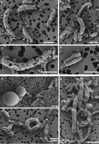
Fig. 5. FE-SEM images of prokaryotic cells from WD samples. (a–d) prokaryotic cells from Termination I (12.3–11.7 ka before 1950 CE), (e–g) prokaryotic cells from Last Glacial Maximum period (23.4–19.9 ka before 1950 CE). White scale bars represent 1 µm.
3.5. Optimization of the fluidic settings on WD ice-core samples: flow rate and pre-filtration
A comparison of three flow rates (14, 32 and 50 µL min−1) revealed no significant evidence of differences in measured cell-densities among the flow rates tested (p-value > 0.1; F-test), implying that the flow rates tested did not have an effect on cell enumeration of WD samples. The flow rates tested did, however, significantly influence the amount of background noise (p-value < 0.01; F-test). The background noise events increased when the flow rate decreased; a flow rate of 14 µL min−1 has a median noise event density 1.71 times larger than a flow rate of 50 µL min−1. We selected a flow rate of 50 µL min−1 to enumerate prokaryotic cells in the WD ice-core samples because it did not significantly influence prokaryotic cell counts, and it provided an adequately low background to detect prokaryotes in samples with low cell concentrations.
The comparison of pre-filtration techniques showed that pre-filtration with a 30 µm filter yielded no significant differences in cell counts from samples that were not pre-filtered (p-value < 0.01; F-test). In contrast, pre-filtration yielded 1.6 times lower background noise than no-pre-filtration. Consequently, samples were always prefiltered through sterile BD Falcon 12mm × 75 mm tubes with 30 µm cell Strainer Cap to prevent clogging of the fluidic system and decrease background noise events.
3.6. Validation of the measurement technique
The minimum detection limit was determined by counting serial dilutions of WD ice-core samples and bacterial cultures with glacial sediments. Four samples were serially diluted (10-fold) to obtain a range of cell densities from ~106 to 100 cells mL−1. Visual inspection of linearity between log-observed and log-expected cell densities indicates that the lowest cell density that could be detected accurately is ~102 cells mL−1 when at least 180 cells are counted by FCM (~1.6 mL sample counted; 32 min) (Fig. 6a).

Fig. 6. Log-scale scatter plots of observed versus expected cell densities used to determine minimum detection limit (a) and accuracy (b) on serial dilutions (with Milli-Q) of WD ice-core samples (X), and samples from bacterial cultures with glacial sediments (∆). Black short-dash line corresponds to the 1:1 log/log relationship (slope = 1 and intercept = 0); red line on (b) corresponds to the accuracy assay log/log linear regression (r
2 = 0.995, p-value < 0.01, ${\hat \beta _0}$
: 0.048 and
${\hat \beta _0}$
: 0.048 and ${\hat \beta _1}$
: 0.985).
${\hat \beta _1}$
: 0.985).
The CV was calculated on 23 random samples with cell concentrations from 102 to 105 cells mL−1. The actual counted cells by FCM were from 182 to 25 307. When using FCM, the estimated CV for cell densities shows a mean of 3.3% with a range of 0.5–6.2%. The 95% CI range for the mean of the CV was (2.6–4.1%), and the 99% CI was (2.3–4.4%); both of them are narrow and do not exceed 5%. The CV is in agreement with the <5% precision calculated for FCM by others (Gasol and del Giorgio, Reference Gasol and del Giorgio2000; Wang and others, Reference Wang, Hammes, De Roy, Verstraete and Boon2010). In addition, we estimated the CV for cell density when using EFM on replicates (5–10) from samples with cell densities between 101 and 103 cells mL−1 (CV > 28%, maximum CV = 72%). As expected, the CV for cell densities when using EFM was higher than when using FCM. The CV for EFM has been reported to be higher (>10%) than FCM at cell densities of 106 cells mL−1 when counting at least 300 cells per filter (Kirchman and others, Reference Kirchman, Sigda, Kapuscinski and Mitchell1982; Kirchman, Reference Kirchman, Kemp, Sherr, Sherr and Cole1993).
To assess accuracy of the FCM protocol, the samples were serially diluted (10-fold) to obtain a density range between 106 and 102 cells mL−1. When comparing log-observed cell densities with the log-expected cell densities, no evidence of differences between log-observed and log-expected cell densities was found (two sided p-value = 0.89, from a two sample t-test). In addition, the log/log linear regression between expected and observed cell densities confirmed a high degree of accuracy for the method; the log/log linear regression showed no deviation from linearity (r 2 = 0.995, p-value < 0.01; Fig. 6b) and the residual plots show random scatter and no systematic trends (data not shown). The estimated slope was 0.985 with a 95% CI range of (0.962–1.001), which is narrow and contains the slope of a 1:1 log/log linear regression (Fig. 6b). The computed intercept was 0.048 with a 95% CI range of [(−0.178) − (0.273)], which includes zero. The estimated log/log linear equation for the observed versus expected bacterial density was:
 $$\eqalign{{\widehat{{\log (y)}}_{\hbox{accuracy assay}}} & = 0.048 + 0.985\;\log (x);\; \cr \quad {\rm SE}({{\hat \beta} _0}) & = 0.110,\;{\rm SE}({{\hat \beta} _1}) = 0.01} $$
3.7. Gating strategy
The final gating strategy was based on the above controls, target cells (non-photosynthetic prokaryotes) and the above protocol assessments, all of which allowed the optimal distinction of DNA-stained non-photosynthetic prokaryotic cells. The six gates we used are described in sequential order. The final gating strategy was validated using 80 WD samples from different depths that were concurrently quantified by EFM. A WD sample is shown as visual examples through the gating strategy description.
Step 1: Gate 1 is a polygon (P1) that removes the background noise inherent to samples and selects the SYTOX positive events (DNA stained events). It is defined using the described blank, background and negative controls. P1 is defined on a density plot of green fluorescence-H (SYTOX-green emission) versus FSC-A channel (Figs 2, 7).

Fig. 7. Cytograms of two WD ice-core samples to select SYTOX-green positive events. Gate 1 (P1, red polygon) is used to include only positive SYTOX-green events and to remove background noise. P1 is defined on a density-plot of green-fluorescence-H (H = height) versus Forward-scatter-A (A = area). (a) Milli-Q as blank control. (b) Background control (0.2 µm filtered stained sample). (c) Negative control (unstained sample). (d): SYTOX-green events from a WD sample. Percentages of events in P1 are presented between parentheses.
Step 2: Gate 2 is a polygon (P2) defined on a dot-plot of green versus red fluorescence (FL3; >670 nm; Fig. 8). Events are acquired from a stained sample and plotted in the dot-plot. That allows for optimal visual differentiation of ‘noise particles’. P2 contains noise events, which have been described as sediments and appear in a diagonal line with relatively more red fluorescence than that for prokaryotic cells (Gasol and others, Reference Gasol, Zweifel, Peters, Fuhrman and Hagström1999; Gasol and del Giorgio, Reference Gasol and del Giorgio2000). Then P2 is gated out from P1, which prevents noise events that can interfere with the counts.

Fig. 8. Cytograms of a WD sample stained with SYTOX-green to select and remove noise particles. (a) Gate 2 (P2), which is defined on a dot-plot of green fluorescence-H (H = height) versus red fluorescence-H (blue laser excitation; FL3) and includes ‘noise particles’ events (diagonal box above the positive SYTOX events). (b–c): Positive SYTOX-green events and P1 on a density-plot of green-fluorescence-H versus forward-scatter-A. (b) Positive control before applying P2 gate. (c) Positive control after gating out P2 events. Percentages of events in each gate are presented between parentheses.
Step 3: Gate 3 is a horizontal marker (M3) defined on a histogram-plot of count versus green fluorescence-H (SYTOX-green) (Fig. 9). M3 is defined as a horizontal marker to discriminate the prokaryotic cluster from cellular debris and eukaryotic cells, which have relatively more green fluorescence than the prokaryotic cluster. In the histogram-plot, the events present in gate P1 (positive SYTOX events) minus P2 events (noise particles) are plotted, and the horizontal marker is drawn around the prokaryotic cluster (Fig. 9).

Fig. 9. Histogram-plots of a WD ice-core samples stained with SYTOX-green and showing gate 3 (M3). M3 corresponds to the red horizontal marker in (b). (a) All events on the stained samples (no gating applied). (b) Gated histogram-plot (P1 events included and P2 events excluded); M3 is defined in the gated histogram-plot to discriminate between the bacterial cluster and cellular debris and/or eukaryotic cells.
Step 4: In order to exclude autofluorescent pigmented prokaryotes and pico-eukaryotes from the prokaryotic cluster, gates 4, 5 and 6 were defined by quadrants (Q4, Q5 and Q6). Pigmented prokaryotes and pico-eukaryotes can have the same sizes and their nucleic acids can also be stained by SYTOX-green. Photoautotrophic pigments are identified using the events in gate M3 (P1 included and P2 excluded), those events are plotted on three plots: (1) FSC-A versus yellow/orange fluorescence (FL2-H, Em. 585 ± 20 nm, Ex. 488 nm) to detect cells with Phycoerythrin (Phy-E; Figs 10a, d); (2) FSC-A versus red fluorescence-blue laser excitation (FL3-H, Em. >670 nm, Ex. 488 nm) to detect cells with autofluorescent chlorophyll-a (Chl-a; Figs 10b, e); and (3) FSC-A versus red fluorescence-red laser excitation (FL4-H, Em. 675 ± 12.5 nm, Ex. 640 nm) to detect cells with Phycocyanins (Phy-C, Figs 10c, f). Q4, Q5 and Q6 are the positive pigment events at each plot, respectively and defined by the upper left (UL) and upper right (UR) quadrant markers at each plot (Fig. 10). After the detection of the autofluorescent events, they are removed from the prokaryotic cluster.

Fig. 10. Cytograms of a WD ice-core sample stained with SYTOX-green and showing gates 4, 5 and 6 (Q4, Q5, Q6). The three cytograms are gated by M3 (see Fig. 9). (a) Detection of Phy-E positive events by quadrant 4 (Q4; upper-left: UL, upper-right: UR). (b) Detection of Chl-a positive events by quadrant 5 (Q5; upper-left: UL, upper-right: UR). (c) Detection of Phy-C positive events by quadrant 6 (Q6; upper-left: UL, upper-right: UR).
Step 5: Finally, prokaryotic density is quantified in gate 3 (M3) after removing gates 4, 5 and 6 (Q4, Q5 and Q6), and plotted in a density-plot of green fluorescence-H versus FSC-A (Fig. 11). As an example, four WD ice-core samples, from different depths that display the final non-photosynthetic prokaryotic events are presented in Figure 11. They show the typical two sub-group pattern of low-nucleic acid content and high-nucleic acid content prokaryotes, which have been discriminated in most aquatic samples (Li and others, Reference Li, Jellett and Dickie1995; Gasol and others, Reference Gasol, Zweifel, Peters, Fuhrman and Hagström1999; Gasol and del Giorgio, Reference Gasol and del Giorgio2000; Lebaron and others, Reference Lebaron2001, Reference Lebaron2002). In contrast to these studies, we observed other subgroups differentiated by green fluorescence throughout the WD samples.
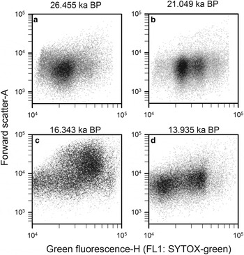
Fig. 11. Cytograms of four WD ice-core samples, stained with SYTOX-green showing final gating with the total prokaryotic cells and subgroups. Those plots include events on M3 and exclude events on Q4, Q5 and Q6. Sample mid-age is on top of each panel.
3.8. Final protocol description
The thresholds are set on the green fluorescence channel (FL1-H) at 750 RIU. Sample (2 mL) is then pipetted using sterile filtered tips from the glass vial to a clean tube with a 30 µm mesh for pre-filtration. From that tube, 150 µL is analyzed as the negative control (unstained sample), and the remaining 1800 µL is stained with SYTOX-green. A background control is obtained from the same sample vial by pipetting 300 µL into a sterile 5 mL syringe attached to a 0.22 µm pore size sterile filter (Millex®-GV4, 4 mm filter units, 0.1 cm2 filtration area), filtered into a falcon tube (12mm × 75 mm, sterile, DNA free), and along with the sample stained with SYTOX-green to a final concentration of 0.05 µm. The samples are then incubated with the stain for 20 min in the dark at room temperature. The samples can be kept at 4°C under these conditions for a period no longer than 20 h before being analyzed by the FCM; after that period, cell counts decrease (data not shown). All samples are then analyzed by FCM using a flow rate of 50 µL min−1 with a core size of 12 µm. We analyzed around 30 samples d−1 based on each sample reaching 25 000 events on gate P1, or until 1600 µL had been analyzed by FCM, which corresponds at 32 min. The samples and controls are analyzed in the following order: 250 µL of blank control, 200 µL for all samples as negative controls (unstained), ~7 background controls of 200 µL (stained 0.2 µm filtered samples), all of which allowed creation of gate 1 (P1). The stained samples are analyzed in random order. To clean the Sample Introduction Probe and prevent a reported slight carry-over between samples (Van Nevel and others, Reference Van Nevel, Koetzsch, Weilenmann, Boon and Hammes2013), two back-flushes are performed and Milli-Q water is run for 1 min between stained samples. Gating strategy is applied after data acquisition is performed.
3.9. Application to WD ice-core samples
To test our FCM protocol, 189 discrete samples of WD ice core were analyzed from 2100 to 2480 m (Fig. 12). That depth range was chosen because we had more sample volume available in this region of the core (4.5–8 mL sample−1), relative to other depths. This volume allowed us to directly observe and count prokaryotic cells by EFM while counting the same samples with FCM. The FCM analysis revealed a mean prokaryotic density of 6.10 × 10⁴ cells mL−1 (range 6.53 × 10³–2.89 × 10⁵ cells mL−1). In addition, the parallel sticks of ice from the same WD ice core were analyzed to test the reproducibility and cleanliness of the melter system (Fig. 12). The replicated samples show the same temporal trends and typically fall within the 95% CI for the means belt of a generalized additive model (GAM) fitted to the data (Wood, Reference Wood2006). Variation in the replicated ice sticks can result from spatial variability in prokaryotic density in the core and possible carry over from previous ice core samples as it is not possible to wash the melter system between each discrete sample.

Fig. 12. Depth record of prokaryote density in the WD ice core using the FCM methods described in this paper. The solid black curve is the fitted model from the optimal quasi-Poisson GAM; the gray areas correspond to the 95% confidence band for means and the white dots are the observed prokaryotic density. Gray stars are parallel replicated ice samples that were melted days and months after the original ice sections by the ice-core melter system. Note the y-axis is on logarithmic scale.
4. DISCUSSION
We developed a protocol for the accurate and precise density measurement of non-photosynthetic prokaryotes archived in the WD ice core. This method is time efficient relative to direct microscopic determination of cell density. Results obtained from the WD ice core using this protocol revealed a unique long-term prokaryotic record that can be used to evaluate non-photosynthetic prokaryotic responses to climatic and environmental conditions.
Mechanical cutting of discrete samples, followed by slow melting at 4°C and ensuing decontamination procedures for microbiological, molecular-based and biogeochemical studies, have significantly increased our knowledge about prokaryotes in glaciers (Sheridan and others, Reference Sheridan, Miteva and Brenchley2003; Miteva and others, Reference Miteva, Sheridan and Brenchley2004; Christner and others, Reference Christner, Mikucki, Foreman, Denson and Priscu2005; Priscu and others, Reference Priscu, Christner, Foreman and Royston-Bishop2007; Segawa and others, Reference Segawa, Ushida, Narita, Kanda and Kohshima2010). However, this traditional melting method is impractical for accessing a prokaryotic record of thousands of years and at high resolution because: (1) sample preparation is laborious, taking ~2 d to clean and processes a section of ice core (~30 cm length); (2) large amounts of sample volume are required to ensure the ice used for analysis is clean; (3) the large sample volume requirement yields samples with low time resolution. In contrast, we used the ice-core melting system, which had for WD ice core a melting rate of ~4 cm min−1 and an average warming rate of ~80 °C min−1, which is faster than the traditional slow mechanical melting method mentioned above (~0.03 °C min−1). It has been demonstrated that slow warming rates (<0.5 °C min−1) are more harmful for prokaryotic and eukaryotic cells than rapid rates (Mazur, Reference Mazur1966; Mazur and Schmidt, Reference Mazur and Schmidt1968; Calcott and MacLeod, Reference Calcott and MacLeod1974, Reference Calcott and MacLeod1975; Calcott and others, Reference Calcott, Lee and MacLeod1976; Parker and Martel, Reference Parker and Martel2002; Walker and others, Reference Walker, Palmer and Voordouw2006). The faster warming/melting rates of the continuous melting system are important for preserving prokaryotic cells and can reduce, or even prevent the recrystallization of intracellular ice, in effect preventing cell damage and lysis (Mazur, Reference Mazur1977; Parker and Martel, Reference Parker and Martel2002; Walker and others, Reference Walker, Palmer and Voordouw2006).
Most previous estimates of non-photosynthetic prokaryotic density in melted ice-core samples relied upon filtration and epifluorescence analysis of stained cells, which are time consuming, can lead to microbial contamination and are plagued by low precision. Analysis via flow cytometer in a clean room allows relatively rapid processing of the samples within a closed fluidic system, eliminating much of the potential for contamination (Gasol and del Giorgio, Reference Gasol and del Giorgio2000; Vives-Rego and others, Reference Vives-Rego, Lebaron and Nebe-von Caron2000; Wang and others, Reference Wang, Hammes, De Roy, Verstraete and Boon2010; Van Nevel and others, Reference Van Nevel, Koetzsch, Weilenmann, Boon and Hammes2013). Sample preparation is rapid (few minutes), and a representative number of cells can be measured in a short time, which allows for the reduction of the baseline variation. The ‘practical minimum detection limit’ in our method is 102 cells mL−1. We deem this a practical detection limit because we did not have sample volumes >8 mL that allowed for higher absolute counts at lower cell densities (<102 cells mL−1). The detection limit by FCM depends on the absolute number of cells counted and sample volume available since counts follow a Poisson distribution, which becomes more regular as the expected number of counts increases (Shapiro, Reference Shapiro2003; Bolker, Reference Bolker2008). For lower prokaryotic densities (<102 cells mL−1), sample volumes >8 mL are needed to obtain accurate and precise counts. In addition, the mean of the CV was 3.34% (range, 0.48–6.2%), which agrees with the estimated precision for FCM by other studies (Gasol and del Giorgio, Reference Gasol and del Giorgio2000; Nebe-von-Caron and others, Reference Nebe-von-Caron, Stephens, Hewitt, Powell and Badley2000; Wang and others, Reference Wang, Hammes, De Roy, Verstraete and Boon2010). In this study, accuracy was demonstrated by serial dilutions of WD samples; the log/log linear relation between observed and expected cell concentrations does not show a deviation from linearity (r 2 = 0.995, p-value < 0.01; Fig. 10b), and 95% CI for both intercept and slope are narrow and contain the values for the 1:1 log/log linear relationship. Cleanliness of the instrument can be easily achieved (Fig. 2; Section 3.1), and a set of FCM controls allows reliability on the positive-target events (Figs 1, 2). Van Nevel and others (Reference Van Nevel, Koetzsch, Weilenmann, Boon and Hammes2013) utilized the same FCM instrument and showed that Milli-Q washes between samples are not necessary when dealing with similar cell concentrations (in the same order of magnitude); because the carry-over accounts for only 0.53% CV of the concentration of the latter sample. We did, however, keep the washing and back-flushing steps to prevent carryover because measurements were performed in random order, and sample cell densities were unknown.
A major challenge of employing FCM to counting prokaryotic cells in natural samples is to find a DNA stain that shows a broad spectral differentiation from autofluorescent particles and minimum non-specific binding (Vives-Rego and others, Reference Vives-Rego, Lebaron and Nebe-von Caron2000). Dust concentrations have been shown to be higher at the LGM than during the Holocene by a factor of ~80 and ~15 in Greenland and Antarctic ice cores, respectively (Fischer and others, Reference Fischer, Siggaard-Andersen, Ruth, Röthlisberger and Wolff2007). The European Project for Ice Coring in Antarctica (EPICA) showed a dust concentration record for the LGM with a mean of 1.95 × 10⁵ particles mL−1 at a sampling frequency of 230 a (Delmonte and others, Reference Delmonte, Petit and Maggi2002). Our results show that SYTOX-green allows spectral differentiation between autofluorescent and DNA stained particles without non-specific binding to abiotic sediments (Fig. 3a), a result that corroborates results of Wobus and others (Reference Wobus2003) and Klauth and others (Reference Klauth, Wilhelm, Klumpp, Poschen and Groeneweg2004).
Although SYTOX-green requires a compromised membrane to enter the cell (Lebaron and others, Reference Lebaron, Catala, Parthuisot and Oce1998a, Reference Lebaron, Parthuisot, Catala and Oceb; Suller and Lloyd, Reference Suller and Lloyd1999; Klauth and others, Reference Klauth, Wilhelm, Klumpp, Poschen and Groeneweg2004), our cell counts obtained with both the EFM and FCM indicate that the cellular membranes in the melted WD samples were already membrane-compromised. The observed ~2-fold reduction of permeabilized prokaryotic cells after fixation (Fig. 4) may result from cell membrane changes caused by formalin (Hopwood, Reference Hopwood1969; Meadows, Reference Meadows1971; Puchtler and Meloan, Reference Puchtler and Meloan1985; Kiernan, Reference Kiernan2000). Melted glacial samples must be preserved to prevent degradation and/or cell growth. We conclude that a reduction in cell density by a factor of ~2 caused by formalin addition is insignificant when our reported prokaryotic density fluctuates between two orders of magnitude (6.53 × 10³–2.89 × 10⁵; Fig. 12).
Compromised membranes can result from lack of source cell integrity, damage during atmospheric transport, and extended exposure to subzero temperatures or during the freeze-thaw processes. Although we do not know the status of the source cells in time, it is known that extensive periods of exposure to subzero temperatures can have a direct effect on membrane lipid conformation and hence, loss of membrane integrity of prokaryotic cells (Mazur and Schmidt, Reference Mazur and Schmidt1968; Calcott and MacLeod, Reference Calcott and MacLeod1975; Mackey, Reference Mackey1984; D'Amico and others, Reference D'Amico, Collins, Marx, Feller and Gerday2006). Prolonged freezing had affected our samples because they were encased in ice from 27 000 to 9600 a before 1950 CE. Undoubtedly, some prokaryotes can remain viable for as long as hundreds of thousands to millions of years when trapped in glacial ice (Christner and others, Reference Christner2000, Reference Christner, Mosley-Thompson, Thompson and Reeve2003; Sheridan and others, Reference Sheridan, Miteva and Brenchley2003; Bidle and others, Reference Bidle, Lee, Marchant and Falkowski2007). Our samples were also exposed to at least one freeze-thaw processes. Calcott and MacLeod (Reference Calcott and MacLeod1974, Reference Calcott and MacLeod1975) and Walker and others (Reference Walker, Palmer and Voordouw2006) showed that freezing and thawing can produce compromised membranes during slow warming and that microorganisms vary greatly in their susceptibility or resistance to the lethal effects of freezing and thawing.
FCM flow rate is a critical parameter impacting the time required to measure samples and the cell detection and/or background noise (Gasol and del Giorgio, Reference Gasol and del Giorgio2000; Shapiro, Reference Shapiro2003). Our cell density comparison at different flow rates showed negligible variations over the flow rates tested. In contrast, background noise decreased with higher flow rates; we showed significant background variations between the lowest flow rate (14 µL min−1) and the other two flow rates tested (32 and 50 µL min−1). Van Nevel and others (Reference Van Nevel, Koetzsch, Weilenmann, Boon and Hammes2013) used the same FCM instrument and showed negligible variations in cell densities between three flow rates (14, 35, 66 µL min−1), choosing 66 µL min−1 to measure prokaryotic densities. We did not test a flow rate of 66 µL min−1; however, an improvement to our protocol could be to increase the flow rate to 66 µL min−1, which will decrease the time per run by a factor of 1.3.
Most studies of water-insoluble impurities in ice cores have reported only their water-insoluble ‘dust’ component (e.g. Ruth, Reference Ruth2003; Fischer and others, Reference Fischer, Siggaard-Andersen, Ruth, Röthlisberger and Wolff2007; Lambert and others, Reference Lambert2008). Our results suggest that prokaryotic cells may also contribute to the water-insoluble impurities, indicating biotic and abiotic particles are preserved in the ice. Hara and Zhang (Reference Hara and Zhang2012) showed that total airborne prokaryotic cell concentrations in Asian dust range from 106 and 107 cells m−3 and were correlated with the concentration of aerosol particles >1 µm. These results, as well as those of others (e.g., Kellogg and Griffin, Reference Kellogg and Griffin2006; Pratt and others, Reference Pratt2009), indicate that bacterial particles can be an important component of atmospheric insoluble particles that can contribute to the ice-core record. Coulter counters or laser particle devices have been used frequently to quantify dust (abiotic particles) in ice cores but they cannot be used with efficacy to quantify prokaryotic cells in large part because cells are substantially smaller than most continental dust particles and often outside the size range of the measurement devices. Because the mass mode of continental dust found in ice cores is in the range, 3–5 µm, very small particles (<1 µm) are generally not the focus of most insoluble dust studies.
Data from Coulter counters are based on the detection of electric signals generated by solid particles that are forced to flow through a small aperture tube in a conductive fluid (NaCl solution). The passage of a cell through the aperture tube results in an increase in resistance by the displacement of its own volume of electrolyte from that region (Kubitschek and Friske, Reference Kubitschek and Friske1986). The sensitivity of this instrument depends on the orifice diameter and electrode size (Harris and Kell, Reference Harris and Kell1985; Sun and Morgan, Reference Sun and Morgan2010). Under controlled laboratory conditions, Coulter counters with smaller aperture tubes (20–30 µm) have been used successfully to quantify bacteria from pure cell cultures (Zimmermann and others, Reference Zimmermann, Pilwat and Riemann1974; Kjelleberg and others, Reference Kjelleberg, Humphrey and Marshall1982; Henningson and others, Reference Henningson, Lundquist, Larsson, Sandström and Forsman1997). For insoluble particle measurements on ice cores, the common aperture diameter is 50 µm (e.g., Ruth and others, Reference Ruth2002; Delmonte and others, Reference Delmonte2004; Lambert and others, Reference Lambert2008; Vallelonga and others, Reference Vallelonga2010), however, 30 µm (Biscaye and others, Reference Biscaye1997) and 20 µm (Steffensen, Reference Steffensen1997) have also been reported. Coulter counters cannot be used to quantify prokaryotes in environmental samples for other reasons. For solid particles, the conductivity is constant under different experimental conditions, whereas the electrical properties of microorganisms change with the magnitude of the applied field, and dielectric breakdown of the membrane has been observed (Zimmermann and others, Reference Zimmermann, Pilwat and Riemann1974, Reference Zimmermann, Groves, Schnabl and Pilwat1980; Harris and Kell, Reference Harris and Kell1985). In addition, the saline solution (NaCl) added to the samples can lead to shrinkage of cells due to osmotic stress, leaving the cells undetected (Csonka, Reference Csonka1989). Consequently, insoluble particles detected by Coulter counters may exclude most of the prokaryotic cells in the sample.
In contrast to Coulter counters, laser particle devices are based on light attenuation and scattering (Ruth, Reference Ruth2002, Reference Ruth2003; Ruth and others, Reference Ruth2002). The sample water is pumped through the detection cell where it is illuminated by a diode laser (670 or 680 nm) with a power of 3 or 7 mW. The size detection limit for laser particle devices is ~1.0 µm of the spherical equivalent particle diameter (Ruth and others, Reference Ruth2002), indicating that the coulter counter can detect a fraction of the prokaryotic size ranges (0.2–3 µm). The detection of prokaryotic cell scattering however, is not easy; it depends upon various factors and requires specialized detectors and light sources. Prokaryotes scatter less light due to their small sizes. This is physically explained by the fact that the scattered light intensity increases as the sixth power of the particle's radius (Salzman, Reference Salzman1999). FCM that are able to detect prokaryotic cells only by scattering are equipped with powerful light sources (~100 mW) of short wavelength because the light scattering detection increases by the square root of the light intensity (Steen, Reference Steen2000), and the scatter intensity decreases as the fourth power of the wavelength (i.e. shorter wavelengths scatter light more strongly) (Salzman, Reference Salzman1999). Thus, to be able to detect prokaryotic cells only by scattering, instruments should have: (1) a powerful laser (>100 mW), (2) a sensitive detector (PTM or avalanche-photodiode instead of a photodiode), (3) light sources of short wavelengths (<600 nm) and (4) low background (Salzman, Reference Salzman1999; Steen, Reference Steen2000). Relative to a laser particle counter, the PhytoCyt FCM has (1) a more powerful light source to measure particle's scattering (20 mW versus 3 or 7 mW for a laser counter), (2) a light source with a shorter wavelength (488 nm versus 670 nm for a laser counter), (3) the same scatter detector (both used photodiodes), and (4) a much lower flow rate (50 µL min−1 versus 20 000 µL min−1 for a laser counter). Despite these differences, our FCM cannot detect prokaryotic cells by scattering alone; prokaryotic scatter typically falls within the equipment noise. Our protocol can discriminate prokaryotic cells based on excitation and emission of a high quantum yield fluorescent DNA stain (SYTOX-green) detected by a PTM tube, which can detect individual photons at low-light levels (weak signals) (Steen, Reference Steen1986, Reference Steen1992, Reference Steen2000; Hadfield, Reference Hadfield2009). In contrast, photodiode detectors gather average light and detect high-light levels (strong signals) (Wood, Reference Wood1997, Reference Wood1998; Shapiro, Reference Shapiro2004). In addition to detector types, particle scattering can be increased by reducing flow velocity; the slower the cells move through the focus the more scattered light they emit and can be detected (Steen, Reference Steen2000). However, laser particle detectors have a higher flow rate than FCM (50 µL min−1 versus 20 000 µL min−1). Consequently, insoluble particles detected by laser particle devices correspond primarily to dust particles whereas FCM can detect accurately fluorescently stained prokaryotic cells.
To evaluate our FCM protocol, we measured prokaryotic density in a short section of WD ice core (Fig. 12). The prokaryotic density record showed changes of two orders of magnitude from 2100 to 2480 m. These depths correspond to Termination I, the period of most recent deglaciation (13 021–19 386 a before 1950 CE), a climatic period with dramatic changes and the largest climatic oscillations of the past 20 000 (Blanchon and Shaw, Reference Blanchon and Shaw1995; Mayewski and others, Reference Mayewski1996; McManus and others, Reference McManus, Francois, Gherardi, Keigwin and Brown-Leger2004). These preliminary results reveal that our method effectively detects prokaryotic cells and that their abundance in glacial ice responds to large-scale ecosystems and/or climatic processes.
ACKNOWLEDGEMENTS
This work was supported by US National Science Foundation (NSF) grants 0440943, 0839075 and 0839093. P. Santibáñez was funded by Chile Fulbright-CONICYT Scholarship. We thank J. D'Adrilli, O. Maselli, M. Sigl, D. Pasteris and others for assistance with ice-core melting and discrete sample collection, M. Skidmore for glacial sediments, C. Foreman and A. Michaud for bacterial isolates and T. Ranalli, T. Vick-Majors, M. Skidmore and A. Chiuchiolo for reading earlier versions of the manuscript. The authors appreciate the support of the WAIS Divide Science Coordination Office at the Desert Research Institute, Reno, NE, USA and University of New Hampshire, USA, for the collection and distribution of the WAIS Divide ice core and related tasks (NSF Grants 0230396, 0440817, 0944348; and 0944266). Kendrick Taylor led the field effort that collected the samples. The National Science Foundation Division of Polar Programs also funded the Ice Drilling Program Office (IDPO) and Ice Drilling Design and Operations (IDDO) group for coring activities; the National Ice Core Laboratory for curation of the core; the Antarctic Support Contractor for logistics support in Antarctica; and the 109th New York Air National Guard for airlift in Antarctica.


 Open access