Introduction

Radio-echo techniques have been used to investigate the physical nature of the Ross Ice Shelf, Antarctica. The data were collected during the 1974–75 austral summer along the series of flight lines shown in Figure 1. Most of these lines run roughly parallel to the ice-shelf front and are separated by a distance of 50 km. Additional flights traced the hypothetical flow lines of ice entering the shelf via streams A and C in the east and Byrd Glacier in the west. Navigation along the specified flight lines was provided by a Litton LTN₅₁ inertial navigation system. This unit gave an overall positional accuracy of six kilometres.

Fig. 1. Ice-thickness and flow-line map. The contour interval is 50 m. Light dashed-dotted lines: flow lines deduced from radio-echo data. Continuous sub-parallel lines: aircraft flight lines.

The radio echo-sounder mounted on board the LC₁₃₀ aircraft was based upon the Technical University of Denmark 60-MHz pulsed radar system. This echo-sounder enables the length of the transmitted pulse to be selected. The shortest pulse, of 60 ns duration, was chosen for work above the ice shelf; it gives a range resolution in ice of 5 m. Typically, the ice shelf was sounded from a height of one kilometre.

Three techniques were used to record the power returned from the ice-shelf surfaces. Two of these recording modes yield the quantitative measurement of echo strength which is required for an investigation of the r.f. dielectric loss in the ice shelf. The most direct method a calibrated A-scope display of the received pulse (Fig. 2- 1). A process of sequence of A-scope frames leads to a value for the dielectric loss. The second recording technique displays the peak of the power returned from the ice-water interface in terms of distance along the flight line. These e.s.m. records (Fig. 2- 2) (Reference NealNeal, 1976) supply information on the small-scale roughness of the ice-water interface as well as on the mean reflection coeficient. The third mode of recording produces the familiar Z-scope photographs (Fig. 2-3). These intensity-modulated range profiles are especially useful for measuring ice thickness.

Fig. 2. 60 MHz A-scope, ESM, and Z-scope records taken from over the Ross Ice Shelf. The letters x, y, and z denote :

x Start of transmitted pulse.

y Return from the ice–air interface.

z Return from the ice–water interface.

Fig. 3. Z-scope record showing an internal reflecting horizon in the ice shelf at position 82° 26´ S., 169° 42´ E. This horizon is believed to delineate a brine percolation layer.

Ice-Thickness and Flow-Line Map

The thickness map shown in Figure 1 has been drawn up from the data obtained in the 1974–75 season. Thickness measurements have been made at roughly one kilometre intervals and the velocity of radar in ice has been taken as 169 m/μs. To correct for the higher velocity in the firn layer, an additional eight metres has been added to the directly computed ice thickness (Reference Robin, Robin, Evans and BaileyRobin and others, 1969). With this correction, the total uncertainty in the thickness is unlikely to exceed eight metres and this includes the digitization error.

A feature commonly recorded on the Z-scope display during a flight over the western side of the ice shelf is shown in Figure 3. This type of return originates from a zone in which brine has percolated horizontally through the porous firn layer after the latter has been penetrated by a bottom crevasse. It is characterized by an occultation of the bottom return and the appearance of the internal reflecting horizon which marks the vertical position of the brine layer. Since brine percolation zones appear to form near the grounding line and can be tracked to the ice-shelf front, they offer an effective means of flow line determination. Indeed, all but one of the flow lines shown in Figure 1 have been so derived. The exception is the line which runs down roughly 180°. This has been deduced from a characteristically abrupt thickness change of 30 m to 40 m. The correspondence between the flow lines of Figure 1 and the velocity vectors measured by Reference ThomasThomas (1976) and Reference Dorrer, Dorrer, Hofmann and SeufertDorrer and others (1969) is very close. A similar agreement exists with the flow lines deduced from indications of streaming by Reference RobinRobin (1975).

The Power Reflection Coefficient of the Ice-Water Interface of the Ross Ice Shelf

The Fresnel reflection coefficient R of an interface illuminated at near normal incidence is related to the intrinsic impedances of the two media by

(1)

Since neither ice nor sea-water are magnetic, the intrinsic impedance η can be expressed in terms of the dielectric constant ∊’ and loss tangent tan δ through

(2)

in which μ ₀ and ∊₀ represent the magnetic permeability and electrical permittivity of free space. These two expressions allow the theoretical reflection coefficient to be calculated.

Values for the permittivity of sea-water and glacial ice are to be found in Reference Smith and EvansSmith and Evans (1972). According to these investigators the relative permittivity of ice at 60 MHz and 0°C is 3.2(1–0.007i). The corresponding value for sea-water is given as 77(1-11.3i). Using these values in conjunction with Equations (1) and (2) gives a power-reflection coefficient of –0.77 dB. This is lowered somewhat if the ice-shelf base consists of frozen sea-water. Assuming that the permittivity is equal to that of the Ward Hunt saline ice (Reference Ragle, Ragle, Blair and PerssonRagle and others, 1964), the reflection coefficient is –0.80 dB.

The remaining possibility which must be considered is that the ice-shelf base probably contains morainal debris. In the absence of documented measurements on the electrical properties of debris-laden ice, the permittivity has been evaluated using Looyenga’s mixture formula (Reference Glen and ParenGlen and Paren, 1975). This relates the permittivity of the mixture ∊_m to those of the ice ∊_i and the rock debris ∊_r by

(3)

in which ν is the fractional volume occupied by the moraine. Reference YevteyevYevteyev (1959) has measured this parameter for debris-laden ice at the base of an ice cliff near Mirny, East Antarctica. He reports a value of less than 12% in the bottommost three metres and this decreases to 4% at five metres above the base. On the basis of this evidence it is assumed that volume fractions in excess of 50% will not be found on the Ross Ice Shelf. This figure is therefore used to compute a lower limit for the reflection coefficient.

The electrical properties of the moraine are taken to be those of the basal rocks upon which the Antarctic ice sheets rest. According to Reference Robin, Robin, Evans and BaileyRobin and others (1969), Antarctic bedrock is thought to be mainly composed of granites and sandstones whose r.f. dielectric constants vary between seven and ten. The loss tangent of these rocks ranges up to, but rarely exceeds 0.03. A lower limit for the reflection coefficient is therefore obtained by adopting a value of 10(1 –0.03i) for the permittivity of the debris. Using this and the prescribed value of 0.5 for the volume fraction, the permittivity of the ice-debris mixture is calculated to be 6.3(1–0.02i). This leads to a reflection coefficient at the sea-water boundary of –1.1 dB.

The reflection coefficient of the ice-water boundary has been shown to be almost independent of any realizable impurity content in the basal layer. A value of –1 dB is therefore adopted for R, and this is expected to hold for a surface of almost arbitrary roughness providing the latter is illuminated with c.w. (continuous wave) radar. The work of Reference NealNeal (unpublished), however, has shown that the use of pulsed radar can lead to a reduction in the value measured for the reflection coefficient when sounding rough surfaces. An estimate of this reduction can be made by evaluating the roughness characteristics of the ice-air and ice-water interfaces. In this way Neal concludes that the effective reduction in R is almost always less than 5 dB.

Neglecting the small transmission loss at the ice-air interface, the bottom-reflection coefficient is equated to the mean received power by:

Reflection coefficient ═ Received power–Geometric loss–Dielectric loss in ice

(4)

P _t and 〈P〉 represent the transmitted power and the mean of the peak received power respectively. The free-space pulse-carrier wavelength is equal to λ and the forward antenna gain is given by G. The terrain clearance and ice thickness are given by h _a and h _i, whilst n represents the refractive index of ice. The dielectric loss imposed on the radar in passing through the shelf has been worked out on the assumption that the ice is free of lossy impurities. The procedure has been to use documented values for the loss tangent (Reference Johari and CharetteJohari and Charrette, 1975; Reference JiracekJiracek unpublished) in conjunction with a derived steady-state temperature profile. The latter represents a numerical solution to the one-dimensional steady-state heat-conduction equation:

(5)

This is derived simply using the assumption that the horizontal strain-rates are independent of depth. The ice-air interface lies in the plane z = 0 and is subject to an annual ice accumulation of A. Melting of the bottom surface, which lies in the plane z ═ H, proceeds at a rate of M metres per year. A value of 40 m²/a has been assigned to K, the thermal diffusivity.

Equation (5) may be solved by specifying the temperature and accumulation melt-rates at both surfaces of the ice shelf. For the purposes of the calculation, the ice–water interface is assumed to lie at the pressure-melting point of sea-water and be subject to a melt-rate of zero. Mean annual surface temperatures and accumulation-rates have been taken from Reference Crary, Crary, Robinson, Bennett and BoydCrary and others (1962).

Measurements of the mean received power were obtained from the e.s.m. records. These have been checked against values deduced from A-scope frames spaced at roughly two-kilometre intervals along flight paths. Except in regions of crevassing, the two sets of measurements invariably agree to within three decibels. In a crevassed zone it is possible for an A-scope frame to coincide with a region of low reflection coefficient which frequently surrounds a bottom crevasse. These anomalous returns are easily spotted and avoided on the e.s.m. records.

Measurement of 〈P〉 enables the reflection coefficient defined in Equation (4) to be computed. Mapping the results out with a contour interval of ten decibels produces the map shown in Figure 4. It is notable that ice streams are well delineated by regional variations of up to 30 dB. Furthermore, the reflection coefficient over large areas of the shelf is much lower than the theoretical prediction. This might indicate an incorrect assessment of the bottom roughness or the presence, within the ice, of an r.f. absorbing impurity.

Fig. 4. Reflection coefficient of the ice-water interface. Contours are at 10 dB intervals.

Open shading: Reflection coefficient greater than 0 dB.

Heavy shading: Reflection coefficient less than –20 dB.

An Interpretation of the Anomalously Low Reflection Coefficients

An uncertainty of up to 3.5 dB exists in the value obtained for 10 log₁₀ 〈P〉/P _t. The error incurred in computing the dielectric loss is thought to be less than 3 dB. Measurements of the reflection coefficient are therefore subject to an error of 5 dB. This means that reflection coefficients of less than –20 dB indicate a mechanism which effectively attenuates the radar by at least 15 dB. The question to be answered is whether or not this loss can result from illuminating a very rough surface with the 60 ns pulse.

Figure 5 shows how the measured reflection coefficient is expected to fall when surfaces of increasing roughness are illuminated from an effective height of 1200 m with a 60 ns pulse. At this terrain clearance the maximum reduction is just over 15 dB. The presence of impure ice is therefore only indicated unambiguously when the reflection coefficient is less than about –20 dB. Reflection coefficients satisfying this criterion presumably result from an attenuation of the radar by a lossy impurity.

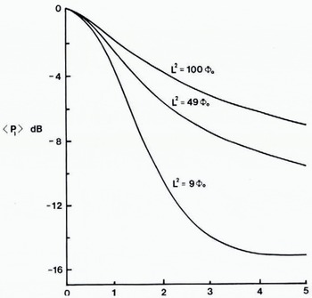
Fig. 5. The mean received power as a function of surface roughness. 〈P ₁〉 is measured relative to the power returned from a perfectly smooth surface at an effective terrain clearance of 1200 m. ϕ₀ represents the r.m.s. phase shift introduced into the radar by the surface roughness. The correlation length L of the roughness has the dimension of metres when ϕ₀ is measured in radians.

Most of the zones of very low reflection coefficient marked in Figure 4 are associated with heavy surface or bottom crevassing. If the firn layer is penetrated by a bottom crevasse, sea-water is able to percolate into the shelf. This phenomenon is well known, and calculations performed by Reference Smith and EvansSmith and Evans (1972) predict a complete occultation of the bottom echo. Figure 3 illustrates the situation which has been previously mentioned. The reflecting horizon within the shelf marks the boundary between the glacial and saline ice which was formed 80 km up-stream near the grounding line of the Beardmore Glacier. Subsequent vertical movement of the ice has depressed the boundary beneath the present firn layer.

Zones a and b of Figure 4 are the only two areas in which a reflection coefficient of less than –20 dB cannot be accounted for by either the brine percolation model or the existence of extensive crevassing. A Z-scope and e.s.m. record taken from within zone a and shown in Figure 6 fail to supply evidence of either pronounced crevassing or an internal reflecting horizon. Moreover, the reflection coefficient of these zones has a tendency to increase towards the ice-shelf front. This is in contrast to the brine-percolation case in which the measured reflection coefficient remains consistently low. The implication is that the impurities found in zones a and b are contained in the bottom few metres of the shelf. Melting of the basal layer as the front is approached is sufficient to produce the observed increase in R ₀.

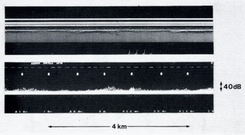
Fig. 6. Z and ESM recordings taken from within the designated zone a at position 79° 48’ S., 174° 00’ E. Aircraft height: 730 m. Ice thickness: 340 m.

The only impurities which are likely to be found in the basal layer are morainal debris or salt. Using the previously computed value of 6.3 (1 –0.2i) for the permittivity of an ice-debris mixture, the dielectric loss is found to equal 0.27 dB/m. D. J. Drewry (personal communication), considers that morainal debris does not in general constitute more than one per cent of the ice thickness. Application of this criterion to a 350 m thick ice shelf gives a loss due to debris of less than 2 dB. This is insufficient to account for the low reflection coefficients of typically –26 dB to –30 dB which arc found in zones a and b.

An estimate of the dielectric loss associated with a layer of sea-water frozen to the ice can be made from the permittivity determined by Westphal for the saline ice on the base of the Ward Hunt Ice Shelf. Reference JiracekJiracek (unpublished) quotes this permittivity as 3.38(1–0.037i) at – 1°C and 150 MHz. Extrapolating to 60 MHz gives a value of 3.43(1–0.050i). The corresponding dielectric loss is 0.51 dB/m. A minimum layer thickness of 10 m is therefore required to account for reflection coefficients down to –30 dB. Comparison with the 120 m of frozen sea-water which Reference MorganMorgan (1972) considered to lie beneath the Amery Ice Shelf shows that 10 m is not an excessive amount. It is, therefore, suggested that the ice-shelf base consists, over zones a and b, of frozen sea-water.

The question of where this sea-water becomes frozen to the base is not easily answered, especially as the process of heat transfer between the ice and water is not well understood. Moreover, knowledge of current flow beneath the shelf is largely restricted to the suggestions of Reference Jacobs, Jacobs, Bruchhausen and BauerJacobs and others (1970) which are shown in Figure 7. In the absence of detailed information, RISP (1974) has proposed a simple model for the prediction of the conditions which favour either bottom melting or freezing. The task is performed by assuming that the sea-water in a boundary layer of specified thickness is always at its pressure-melting point. To satisfy this requirement, water which flows in the direction of a thickening shelf must cool down. If the heat lost by conduction through the ice is insufficient to maintain the necessary cooling rate, then bottom melting will occur. Conversely, freezing takes place when the sensible heat transferred to the shelf exceeds that dissipated by the boundary layer. In this way a ten-metre boundary layer moving at a speed of one centimetre per second parallel to the thickness gradient produces bottom melting when the gradient exceeds 3 × 10^–4. Gradient values lower than this are associated with areas of potential bottom freezing. As pointed out by RISP, the magnitude of the critical gradient is strongly dependent on the values assigned to the thickness and velocity of the boundary layer. Nevertheless, the calculation brings out the significance of the thickness gradient for those areas which are subject to a preferred direction of current flow.

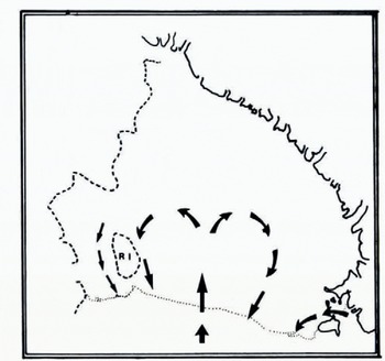
Fig. 7. The suggestions of Reference Jacobs, Jacobs, Bruchhausen and BauerJacobs and others (1970) for the current flow beneath the Ross Ice Shelf. Adapted from figure 4 of RISP (1974)

Referring to the thickness map of Figure 2, it can be seen that zones a and b lie in a relatively flat wedge of thin ice. Along the eastern edge of zone b, the thickness gradient increases from 5 × 10^–4 at 80^° 30’ S. to 2.5 × 10^–3 at 83^° S. Similarly, gradients of up to 1.6 × 10^–3 are found on the eastern side of zone a. These represent ideal conditions for freezing the east–west current gyre. Moreover, the flat profile of the wedge will act so as to prevent subsequent melting even if the current should reverse its direction. To the west of these zones, positive thickness gradients limit an extension of the freezing locale. In the light of this discussion, it is not unreasonable to suggest that bottom freezing is taking place south of 80^° S. in these two zones.

An Interpretation of Reflection Coefficients Which Lie Between – 10 DB and – 20 DB

There are three major areas over which the reflection coefficient falls between –10 dB and –20 dB. These are labelled c, d, and e on the map of Figure 4. Providing the interpretation of surface roughness characteristics is correct, and allowing a two-decibel loss for morainal material, a reflection coefficient of less than –12 dB indicates saline ice.

Figure 8 presents an e.s.m. and Z-scope recording taken from within zone c at position 80^° 27’ S., 179° 2’ E. The measured reflection coefficient is –16 dB. A loss of at least four decibels is therefore attributable to the saline ice which, in the absence of pronounced crevassing, is believed to be frozen to the base. This finding is not too surprising since zone c is, as far as an east–west current is concerned, an area of high negative thickness gradient. To account for a loss of four decibels it is necessary to postulate a minimum layer thickness of four metres.

Fig. 8. Z-scope and ESM recordings taken from position 80° 27’ S., 179° 02’ E. inside zone c. Aircraft height: 890 m. Ice thickness: 330 m.

A section of an e.s.m. and Z-scope recording taken from within zone d are shown in Figure 9. The measured reflection coefficient is –17 dB and, once again, a basal layer of saline ice is indicated. This can be reconciled with the thickness-gradient model by noting that the ice shelf in zone d is almost flat. No difficulty is posed by the channels of low reflection coefficient to the east and west of zone f. These are thought to result not from bottom freezing, but rather from the presence of surface crevasses. The scattering which these produce lowers the mean power received from the ice-water interface. This in turn leads to a low value for R ₀.

Fig. 9. Z-scope and ESM recordings taken from within zone d at position 80° 32’ S., 177° 00’ W. The strong return towards the centre of the record corresponds to a slight increase in ice-shelf thickness and is believed to indicate an area of local bottom melting. Aircraft heigh : 880 m. Ice thickness : 365 m.

A similar explanation is proposed for the low reflection coefficient area, zone e. In this case the crevasses were probably formed in the Stearshead region. Their closure as the ice streams northwards limits the extent of zone e.

The remaining zones in which the reflection coefficient lies between –10 dB and –20 dB are associated with the glacier outflow streams on the western side of the shelf. Once again, saline impurity is believed to be present although it is not possible to conclude with confidence that bottom freezing is occurring. The ambivalence results from the close proximity of brine percolation zones.

An Interpretation of Positive Reflection Coefficients

The phenomenon of positive reflection coefficients arises from the assumption of zero bottom melt-rate which was made in the computation of the dielectric loss. Specifying a non-zero melt-rate changes the temperature profile and hence the dielectric absorption. A positive melt-rate increases the downward advection of ice. This lowers the mean temperature of the ice column which results in a decreased dielectric loss. Conversely, bottom freezing raises the mean column temperature by reducing the downward transportation of cold ice. The situation is well illustrated by the temperature profiles of Figure 10. These represent solutions to Equation (5) for the three bottom melt-rates of 0 m/a and ±0.15 m/a. The ice thickness, top surface temperature, and accumulation-rate have been chosen to match those found at the RISP J-9 bore-hole site (82° 22’ 30″ S., 168° 37’ 33″ W.). It is seen that the temperature profile is strongly dependent on the melt-rate. This dependence is sufficient to produce a difference of four decibels in the two-way dielectric loss computed for curves A and C.

Fig. 10. Theoretical steady-state temperature profiles derived from Equation (computed to be 4) for the RISP J-9 bore-hole site. The three curves, A, B, and C, correspond to annual bottom melt-rates of 0.15 m, 0 m, and –0.15 m of ice. The measured profile, represented by the series of point values, suggests a melt-rate close to 0 m per year.

It is interesting to compare the theoretical curves with the temperature profile which has been measured over the first 100 m (Reference RandRand, 1975). A simple matching suggests that the melt-rate at J-9 is close to zero. Strain-rate measurements carried out as part of the RISP programme had led Reference Thomas and GaylordThomas and Gaylord (1974) to a similar conclusion. J-9 lies in an area over which the reflection coefficient is compatible with the theoretical value deduced earlier. This observation is consistent with the requirement that areas of “normal” reflection coefficient should be free of saline impurities.

An explanation has now been provided for the positive reflection coefficients measured in the north-western sector of the shelf. To account for values of up to five decibels it is necessary to postulate melt-rates of up to 1.5 m/a near the ice-shelf front. This is somewhat lower than the 1.99 m/a deduced by Reference Crary, Crary, Robinson, Bennett and BoydCrary and others (1962) for an area to the south-east of Ross Island. Their deduction was, however, based on a mass-balance study. This technique was also used by Reference PaigePaige (1969) who records a melt-rate of 1.06 m/a on the McMurdo Ice Shelf.

It can be seen by reference to Figure 11 that the two areas in which bottom melting is known to occur are associated with a very smooth ice-water interface. Moreover, all but one of the areas with a smooth bottom are associated with high thickness gradients conducive to bottom melting. It is therefore suggested that bottom melting produces a smooth ice-water interface. Figure 11 is believed to delineate regions of bottom-surface ablation.

Fig. 11. Roughness characteristics of the ice-water interface. Zones in which the roughness of the ice-water interface is less than that of a typical crevasse-free ice-air interface are denoted by heavy shading.

If, as proposed, a smooth ice-water interface is indicative of bottom melting, then it is pertinent to ask why positive reflection coefficients are only measured in the north-western sector of the ice shelf. Two explanations are available: The first suggests that the melt-rate is insufficient to affect the dielectric absorption noticeably. While this situation may well exist in the central and southernmost parts of the ice shelf, the work of Reference Crary, Crary, Robinson, Bennett and BoydCrary and others (1962) indicates appreciable melt-rates in the vicinity of Roosevelt Island. The lack of positive reflection coefficient in this area is thought to arise from the finite time required by the ice shelf to re-establish a steady-state condition following an increase in bottom melt-rate. This time period is a rapidly increasing function of ice thickness and is measured in tens or hundreds of years. The ice shelf therefore acts as a low-pass temperature filter in which the output response is delayed with respect to melt-rate changes at the input. An estimate of bottom melting made during the response time by equating the observed dielectric loss to a value derived from a steady-state temperature profile will thus be lower than the true value. It is assumed that the thick ice around Roosevelt Island imposes a response time which is large enough to prevent the detection of bottom melting along the northernmost flight path.

Further Evidence in Support of a Basal Layer of Saline Ice

It has been argued that the low bottom reflection coefficients, measured over several regions of the shelf, result from the dielectric loss imposed by a basal layer of saline ice. The reflection coefficient of the boundary between the glacial and saline ice is computed to be –38 dB. This is large enough to allow the detection of the returned power.

An example of what is believed to be a return from the saline ice boundary is shown in the Z- and A-scope records of Figure 12. These were made at position 79° 56’ S., 177° 0’ E., which lies in zone b. Careful examination of the Z film reveals an intermittent reflecting horizon just above the ice-water interface. The strength of this return, which is barely resolved on the A-scope frame, indicates a reflection coefficient of around –38 dB. This is in good agreement with the theoretical prediction. The fact that the return from the saline ice is only just resolved implies a maximum layer thickness of five metres. This is reasonably close to the minimum value of eight metres required to account for the measured bottom reflection coefficient of –28 dB.

Fig. 12. Z-scope and A-scope records from position 79° 56’ S., 177° 10’ E. in zone b. An intermittent reflecting horizon, arrowed, just above the ice shelf base is thought to indicate a glacial-ice-saline-ice boundary.

Summary

Detailed analysis of radio-echo data has resulted in a regional evaluation of the r.f. dielectric loss of Ross Ice Shelf ice. Comparison with theoretical loss values, computed under the assumption of steady-state conditions and zero bottom melt-rate, has enabled areas of potential bottom melting and freezing to be delineated. It appears that the rates of bottom freezing are probably too small to be deduced from surface strain-rate-velocity measurements. There is some evidence to suggest that bottom melting produces a smooth ice-water interface. This observation provides a tentative but quick method for recognizing areas of bottom melting on floating ice masses.