

1. INTRODUCTION
Satellite gravity and satellite altimetry missions have collected numerous reliable observations for the study of the mass balance of the Antarctic Ice Sheet (AIS) over the past decade. Changes in ice mass can be deduced from temporal gravity changes from satellite gravity missions, such as the Gravity Recovery and Climate Experiment (GRACE) (Velicogna and Wahr, Reference Velicogna and Wahr2006), or from the combination of temporal surface height changes from satellite altimetry missions, such as the Ice, Cloud and Land Elevation Satellite (ICESat) (Ewert and others, Reference Ewert, Groh and Dietrich2012). However, ice mass changes derived from these observed datasets are inevitably affected by glacial isostatic adjustment (GIA). Generally, the influence of GIA is estimated and removed using a GIA model. However, current GIA models have considerable uncertainties on the same scale as the estimated ice mass change. The lack of data is one issue, and questions regarding the shallow earth structure are another (Morelli and Danesi, Reference Morelli and Danesi2004; Larter and others, Reference Larter2007; Groh and others, Reference Groh2012; Gunter and others, Reference Gunter2014). This uncertainty will lead to large uncertainties in the final ice mass change estimates from satellite missions (Riva and others, Reference Riva2009; Groh and others, Reference Groh2012; Gunter and others, Reference Gunter2014).
To overcome this problem, several studies have proposed combining GRACE and ICESat datasets to determine the GIA over the AIS (Wahr and others, Reference Wahr, Wingham and Bentley2000; Velicogna and Wahr, Reference Velicogna and Wahr2002; Riva and others, Reference Riva2009; Groh and others, Reference Groh2012; Gunter and others, Reference Gunter2014). Wahr and others (Reference Wahr, Wingham and Bentley2000) developed an iterative method in the spectrum domain to combine the two datasets to determine the GIA. The iterative method was later improved by Velicogna and Wahr (Reference Velicogna and Wahr2002), with the inclusion of GPS vertical crustal deformation rates as an additional constraint. Riva and others (Reference Riva2009) developed a single step approach in the spectral domain to combine the two datasets to determine the GIA. This approach was used by Groh and others (Reference Groh2012) for the Amundsen Sea Embayment (ASE) sector of the West Antarctica Ice Sheet (WAIS). More recently, Gunter and others (Reference Gunter2014) incorporated the impact of firn densification on surface height changes within the ICESat data. In this study, we introduce GPS vertical deformation rates and an iterative algorithm in the spatial domain to the method of Gunter and others (Reference Gunter2014). GIA, ice mass change and corresponding elastic vertical crustal deformation are simultaneously computed, incorporating both GPS data and the firn densification model, creating a self-consistent set of estimates.
A total of 379 subglacial lakes have been found beneath the AIS (Wright and Siegert, Reference Wright and Siegert2012). They can be classified as active and inactive subglacial lakes. Smith and others (Reference Smith, Fricker, Joughin and Tulaczyk2009) identified 124 active subglacial lakes (ASLs) beneath the AIS using ICESat data. Due to water filling and draining in these ASLs, the height of the ice-sheet surface may change over the spatial areas of these ASLs, and it can be observed by ICESat (Fricker and others, Reference Fricker, Scambos, Bindschadler and Padman2007; Sergienko and others, Reference Sergienko, MacAyeal and Bindschadler2007; Smith and others, Reference Smith, Fricker, Joughin and Tulaczyk2009). However, the presence of these ASLs means that the height change of the ice-sheet surface is not proportional to the mass change of the corresponding areas, which is observed by GRACE. In addition to water movement, the mass change is also caused by ice motion, which includes asynchronous ice-sheet surface and ice-bottom displacement. Ice-sheet surface displacement during and after lake drainage is as much as 60% smaller than the corresponding ice-bottom displacement, and ice-sheet surface motion continues for some years after the end of water movements (Sergienko and others, Reference Sergienko, MacAyeal and Bindschadler2007; Smith and others, Reference Smith, Fricker, Joughin and Tulaczyk2009). This means that the surface change rates above ASLs derived from ICESat data do not match with the mass change rates of the corresponding regions derived from GRACE data. The mismatch will lead to errors in GIA estimates from combined satellite datasets. This issue is addressed through additional processing of ICESat data. To the best of our knowledge, this is the first time that the influence of ASLs on GIA estimates from combined GRACE and ICESat datasets is considered.
This study focuses on the ice sheet inside the ice grounding lines (Zwally and others, Reference Zwally, Mario, Matthew and Jack2012a) north of 86°S (as the ICESat satellite observations cover only to 86°S). Present-day GIA, ice mass changes and corresponding elastic vertical crustal deformation over these regions are estimated simultaneously by utilizing 6-year GRACE and ICESat observations (from October 2003 to October 2009).
2. DATASETS
2.1. Surface height change rates derived from ICESat
In our investigations, the surface height change rates were derived from the latest release of ICESat data (GLA12, Version 34), which were provided by the National Snow and Ice Data Center (NSIDC) and covered the time span from September–November 2003 to September–October 2009 with a 91-day repeat orbit (Zwally and others, Reference Zwally2012b). Standard quality flags and other criteria, such as the use of measurements with only a single peak in the return echo, a maximum gain value of 200 and a maximum variance of waveform from the Gaussian of 0.04 V, are used in the pre-processing of ICESat data to cull and correct the measurements prior to the computation of surface height change rates. After data pre-processing, the surface height change rates over the AIS are calculated using a repeat-track analysis approach by fitting the surface height measurements in an area of 700 m × 500 m along the repeat tracks to a mathematical model from Ewert and others (Reference Ewert, Groh and Dietrich2012). The campaign bias is calculated using the surface height measurements obtained in the most arid region of East Antarctica, similar to Gunter and others (Reference Gunter2014), with accumulation or compaction considered using the Institute for Marine and Atmospheric Research Utrecht Firn Densification Model (IMAU-FDM) (Ligtenberg and others, Reference Ligtenberg, Heilsen and van de Broeke2011). The trend on the bias estimates is 1.34 ± 0.06 cm a−1. It is removed from all surface height change rates uniformly. Then, we project the locations of the surface height change rates to the polar stereographic projection coordinate system. Within the polar stereographic projection coordinate system, a grid with a spatial resolution of 20 km × 20 km is generated from the median of all surface height change rates within the corresponding grid cell, as shown in Figure 1a. The median values are used instead of the more common mean values because the former yields a more robust solution for each grid cell than the latter with respect to the presence of outliers (Claerbout and Muir, Reference Claerbout and Muir1973; Ewert and others, Reference Ewert, Groh and Dietrich2012). The standard deviation derived from the post-fit residuals at each 20 km × 20 km cell by least squares fitting is used as the corresponding uncertainty of the surface height change rate derived from ICESat data, as shown in Figure 1b.
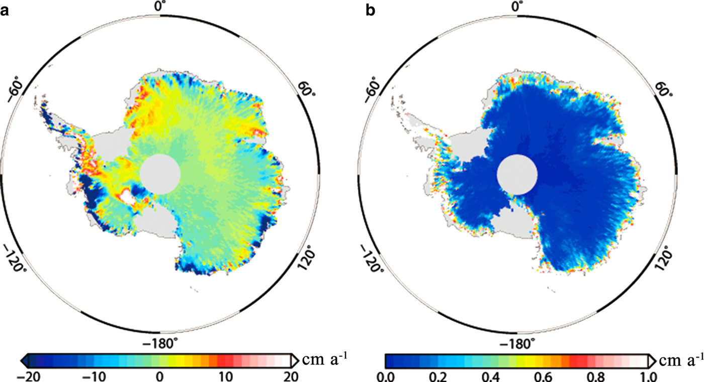
Fig. 1. (a) Surface height change rates and (b) uncertainties over the AIS derived from ICESat data.
To address the mismatch between surface change rates derived from ICESat data and the mass change rates of the corresponding regions derived from GRACE data caused by ASLs, we remove ICESat observations above active lakes before surface height change rates are calculated. The boundary data of these ASLs are obtained from Smith and others (Reference Smith, Fricker, Joughin and Tulaczyk2009). A total of 569035 observations are removed, accounting for only 0.4% of the total ICESat observations. The removal of these observations does not affect the generation of the 20 km × 20 km grid. Note that impacts of inactive subglacial lakes are not discussed in this study because these lakes are generally considered steady. This subject matter is an interesting area of future research.
2.2. Mass change rates derived from GRACE
Mass change rates are derived from GRACE RL05 monthly gravity field solutions provided by the Center for Space Research (CSR). The solutions in the spherical harmonic domain are up to 60°. The C20 coefficient is replaced with that derived from Satellite Laser Ranging (SLR) (Cheng and others, Reference Cheng, Tapley and Ries2013). Degree one coefficients are added back using the values produced by Swenson and others (Reference Swenson, Chambers and Wahr2008). A de-striping filter P3M6 (Chen and others, Reference Chen, Wilson, Tapley and Grand2007) and a 400 km Gaussian smoothing filter are used to weaken and eliminate the impacts of the ‘striping’ and higher order noise. The leakage-in error is reduced using the approach proposed by Wahr and others (Reference Wahr, Molenaar and Bryan1998). The calculation procedure is as follows: (1) The global mass without the AIS is determined from GRACE. (2) The spherical harmonic coefficients caused by that mass are calculated. (3) These spherical harmonic coefficients can be removed from the original GRACE data to obtain an estimate of the AIS mass contributions. (4) Mass change rates over the AIS with the leakage error corrected are obtained from mass contributions. Scaling factors are multiplied by GRACE estimates to restore the amplitude dampening (Velicogna and Wahr, Reference Velicogna and Wahr2006; Gao and others, Reference Gao, Yang, Zhang, Shi and Zhu2015). The scaling factor is calculated as follows: (1) we construct a uniform 1-cm water mass change spread evenly over the AIS. (2) We convert it to spherical harmonic coefficients and filter it in the same way as GRACE data, i.e., truncating it to 60° and by order and applying a 400 km Gaussian smoothing filter, to estimate the filtered results. (3) The scaling factors are estimated by 1 divided by the filtered results. By using the above-mentioned process, the spherical harmonic coefficients are converted into monthly equivalent water height time series on grids with a spatial resolution of 0.25° × 0.25°. Thereafter, the mass change rate, as shown in Figure 2a, at each grid points is obtained by fitting the time series to a mathematical model, which includes linear trends, seasonal changes, and S2 and K2 tides. Uncertainties of the mass change rates, as shown in Figure 2b, are estimated from the calibrated errors for the spherical harmonic coefficients provided by the CSR, and standard deviations of degree one and C20 coefficients are provided with the corresponding coefficients using formal error propagation techniques.
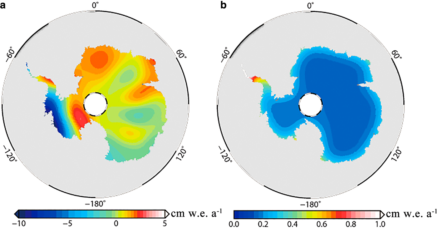
Fig. 2. (a) Mass change rates and (b) uncertainties over the AIS derived from GRACE data.
2.3. Firn densification model and surface mass balance (SMB)
Surface height change rates derived from ICESat data are associated with both mass-conserving (firn compaction) and mass-changing (deposition and removal) processes (Zwally and others, Reference Zwally2005; Gunter and others, Reference Gunter2014; McMillan and others, Reference McMillan2016). To convert surface height change rates derived from ICESat data into mass change rates, the surface height rates derived from IMAU-FDM are subtracted from the surface height rates obtained from ICESat data. IMAU-FDM is forced at the upper boundary with 6-h surface temperatures, accumulation and melting from RACMO2.3 regional climate modelling (Lenaerts and others, Reference Lenaerts, Den Broeke, Berg, Meijgaard and Kuipers2012). The surface height rates and uncertainties derived from IMAU-FDM over the study period (from October 2003 to October 2009) are shown in Figure 3. According to Ligtenberg and others (Reference Ligtenberg, Heilsen and van de Broeke2011), however, surface height rates derived from IMAU-FDM not only contain the surface height change rates due to firn compaction but also include the surface height change rates due to SMB variations that are related to mass gains (precipitation) and mass losses (surface runoff, sublimation and drifting snow erosion) of firn. Therefore, we need to add SMB mass change rates back. In this study, SMB mass change rates are derived from RACMO2.3 simulations of SMB provided by the Institute for Marine and Atmospheric Research Utrecht (IMAU) during the study period. The SMB mass change rates are shown in Figure 4a.
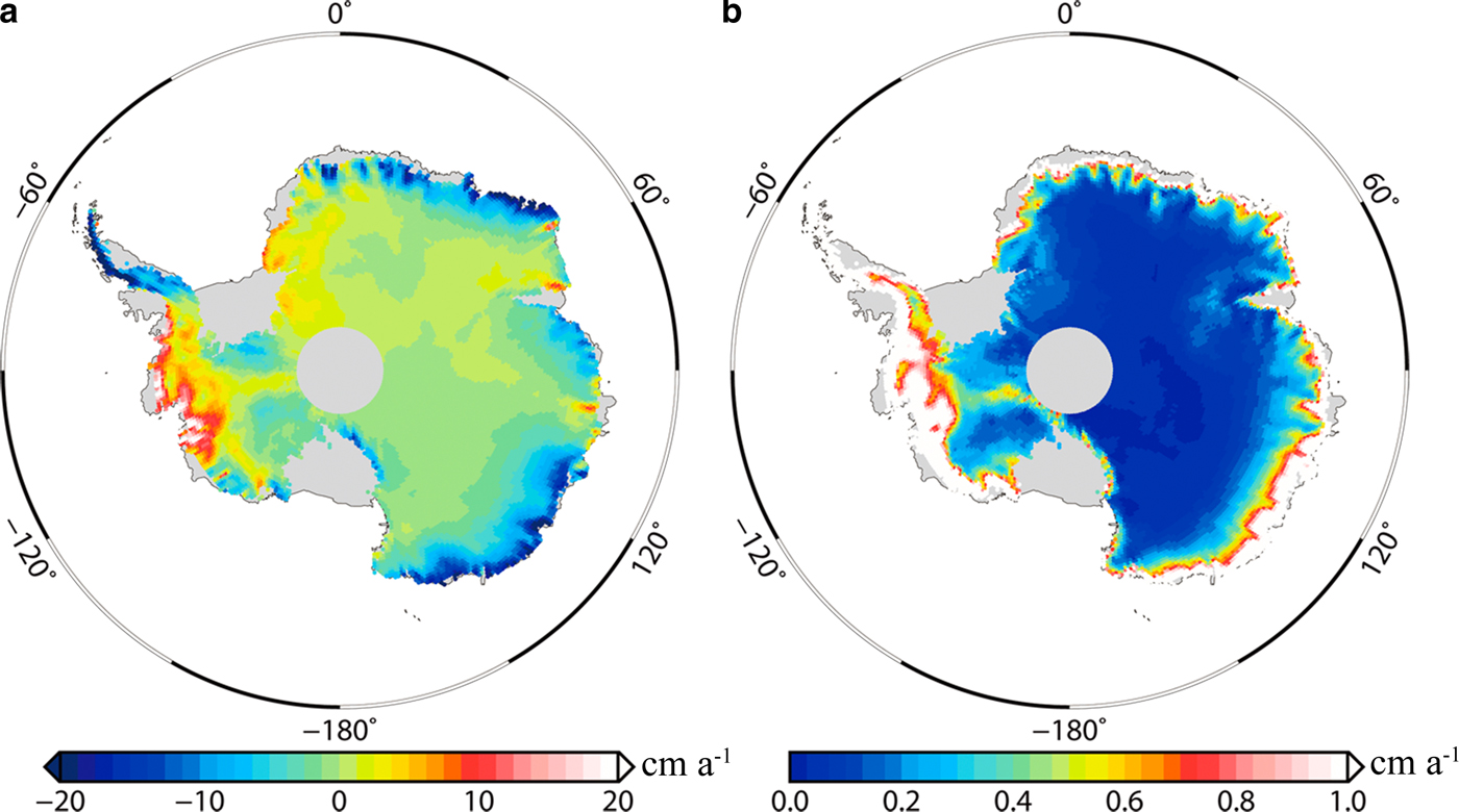
Fig. 3. (a) Surface height change rates and (b) uncertainties over the AIS derived from IMAU-FDM.
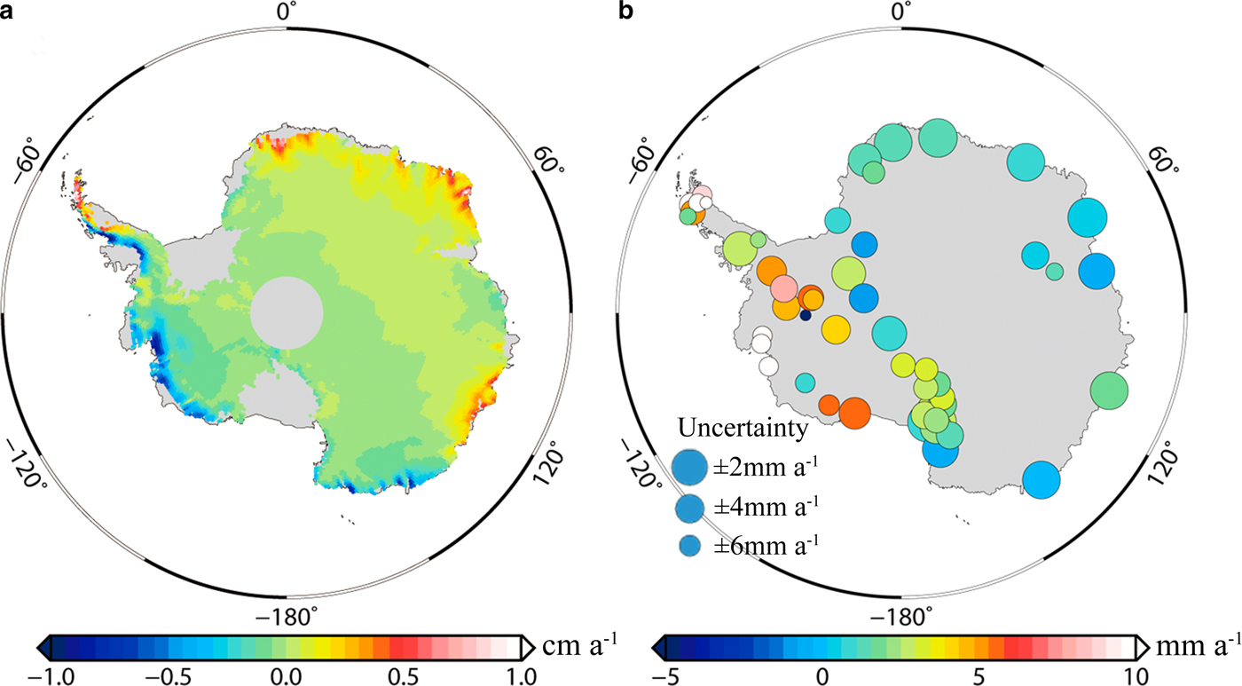
Fig. 4. (a) Mass changes rates due to SMB derived from RACMO2.3 and (b) vertical crustal deformation rates derived from GPS sites. The larger the circle is, the more certain the estimate.
2.4. Ice/snow density model and rock layer density model
Surface height change rates can be converted to mass change rates by multiplying the results by a density model of ice/snow lost or gained. In this study, the density model of the ice/snow lost or gained is determined using the method proposed by Gunter and others (Reference Gunter2014), as shown in Figure 5a. The density model is constructed based upon assumptions that were defined to account for the differences between the surface height change rates derived from ICESat data and those derived from IMAU-FDM. If the differences are negative and greater than the twofold uncertainties of the surface height change rates derived from ICESat data and FDM, they are assumed to be the result of ice dynamics (glacier thinning), and the density assigned to this ice/snow loss is that of ice. If the differences are positive and greater than the twofold uncertainties of the surface height change rates derived from ICESat data and FDM, they are assumed to be attributed to an underestimation of SMB by RACMO2.3 and given a density closer to that of snow using a static density profile similar to that of Kaspers and others (Reference Kaspers2004). If the differences fall within the twofold uncertainties of the surface height change rates derived from ICESat data and FDM, then the height measurements are considered to be within the uncertainty of the datasets, and the mass of the difference is neglected. Details can be found in Section 3.3 of Gunter and others (Reference Gunter2014).
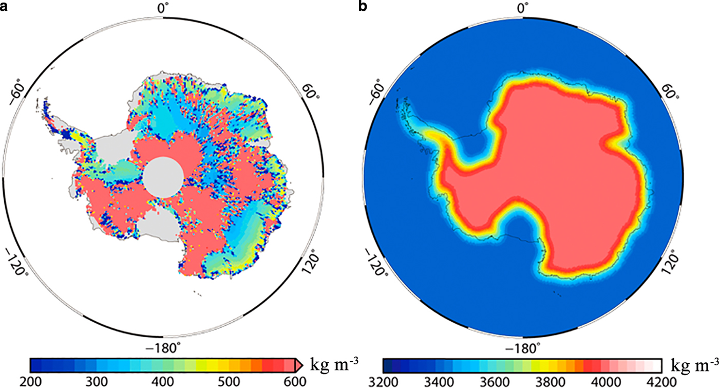
Fig. 5. (a) Density model of the ice/snow lost or gained and (b) density model of the rock layer model.
The rock layer density, as shown in Figure 5b, is derived from the effective rock density model constructed by Riva and others (Reference Riva2009). It is assumed that the rock layer density varies smoothly from 4000 kg m−3 for land to 3400 kg m−3 under ice shelves. These values are refined based on the ratio between mass changes and topography changes induced by GIA and comparison of forward model results obtained from different combinations of parameters. Details can be found in Section 3.1 of Riva and others (Reference Riva2009).
2.5. Vertical crustal deformation rates derived from GPS
Vertical crustal deformation rates for up to 64 GPS sites are listed in Argus and others (Reference Argus, Peltier, Drummond and Moore2014). We use 52 of them to constrain the combined results. In this study, we call the results derived from combining satellite datasets as the combined results. The 52 GPS vertical crustal deformation rates are shown in Figure 4b. Listed below is the reason for the removal of sites and additional required processing.
(1) Seven GPS sites located in the Erebus Mount region located in West Antarctica may be affected by volcanic activity. Therefore, their rates are not used to constrain the combined results in this paper.
(2) In the Northern Antarctic Peninsula, elastic vertical crustal deformation rates abruptly increased in response to the abrupt ice mass loss following the breaking u of the Larsen B Ice Shelf in February 2002 (Thomas and others, Reference Thomas2011; Argus and others, Reference Argus, Peltier, Drummond and Moore2014). The vertical crustal deformation at five GPS sites (O'Higgins, Palmer, Rothera, Frei, and smrt) located in the Northern Antarctic Peninsula was derived from observations before and after the abrupt increase in the ice mass loss. This abrupt ice mass loss will generate an abrupt increase in the elastic vertical crustal deformation at these sites. As such, they will not be used in the study.
(3) The mass change rates in the ASE abruptly increase by 123 Gt a−1 in 2008, resulting in an abrupt increase in the elastic vertical deformation across this region (Argus and others, Reference Argus, Peltier, Drummond and Moore2014). The vertical deformation rates derived at the three GPS sites (bear, mant and pig2) across this region contain observations from this period and need to be corrected for this abrupt increase. To preserve the three GPS vertical crustal deformation rates to constrain the combined results, the differences of elastic vertical crustal deformation between the period of the combined results and the period of these three GPS vertical crustal deformation rates are calculated from GRACE data and corrected to these three GPS vertical crustal deformation rates.
3. METHODOLOGY
3.1. Combination strategy
According to Wahr and others (Reference Wahr, Molenaar and Bryan1998), mass change rates  $\dot m_{{\rm GRACE}} $, which are calculated from GRACE data as mentioned in Section 2.2, can be decomposed into the following components:
 $$\dot m_{{\rm GRACE}} = \dot m_{{\rm ice}} + \dot m_{{\rm GIA}} $$
where  $\dot m_{{\rm ice}} $ denotes ice mass change rates and $\dot m_{{\rm GIA}} $ represents GIA-related mass change rates. Surface height change rates $\dot h_{{\rm ICESat}} $ are calculated from ICESat observations as mentioned in Section 2.1. $\dot h_{{\rm ICESat}} $ is composed of height change rates of firn ( $\dot h_{{\rm firn}} $), thickness change rates of ice ( $\dot h_{{\rm ice}} $), GIA-related vertical crustal deformation rates ( $\dot h_{{\rm GIA}} )$ and elastic vertical crustal deformation rates ( $\dot h_{{\rm ela}} )$ (Riva and others, Reference Riva2009). Thus,
 $$\dot h_{{\rm ice}} = \dot h_{{\rm ICESat}} - \dot h_{{\rm firn}} - \dot h_{{\rm GIA}} - \dot h_{{\rm ela}}. $$
 According to Section 2.3,  $\dot m_{{\rm ice}} $ can be derived from
 $$\dot m_{{\rm ice}} = \dot h_{{\rm ice}} \rho _\alpha + \dot m_{{\rm firn}}, $$
where ρ α is determined using the method proposed by Gunter and others (Reference Gunter2014) as mentioned in Section 2 and  $\; \dot m_{{\rm firn}} $ is the SMB mass change rates derived from RACMO2.3 simulations of SMB. GIA-related mass change rates can be derived as
 $$\dot m_{{\rm GIA}} = \dot h_{{\rm GIA}} \rho _{{\rm rock}}, $$
where ρ rock denotes the density of the rock layer, introduced in Section 2.4. Therefore, substituting  $\dot m_{{\rm ice}} $ into Eqn (1) by (3) and replacing $\dot m_{{\rm GIA}} $ in Eqn (1) by (4), we obtain the following:
 $$\dot h_{{\rm GIA}} = \displaystyle{{\dot m_{{\rm GRACE}} - (\dot h_{{\rm ice}} \rho _\alpha + \dot m_{{\rm firn}} )} \over {\rho _{{\rm rock}}}}. $$
 According to Groh and others (Reference Groh2012),  $\dot h_{{\rm ela}} $ can be derived from the following:
 $$\dot h_{{\rm ela}} = \displaystyle{{h_n} \over {2n + 1}}\displaystyle{{4\pi a^3} \over M}\dot m_{{\rm ice}}, $$
where a and M denote the spherical radius and mass of the Earth and h n denotes load Love numbers of degree n. $\dot h_{{\rm GIA}} $ occurs on both sides of Eqn (5). When $\dot h_{{\rm ela}} $ is calculated by Eqn (6), $\dot h_{{\rm GIA}} $ needs to be known first. Thus, an iterative process is required to estimate $\dot h_{{\rm GIA}} $ by Eqn (5). Initially, we assume the surface height change derived from ICESat data and the ice mass change derived from GRACE data are sensitive only to ice/snow changes and not sensitive to GIA, i.e., $\dot h_{{\rm GIA}} $ = 0. We refer to this as the initial iteration. Thereafter, we repeat the process: first, calculate $\dot m_{{\rm ice}} $ by Eqn (1); second, calculate $\dot h_{{\rm ela}} $ by Eqn (6); third, calculate a new $\dot h_{{\rm GIA}} $ by Eqn (5); and, fourth, calculate $\dot m_{{\rm ice}} $ by Eqn (1) using the new $\dot h_{{\rm GIA}} $. This procedure is repeated until the improvement is negligible. The estimations of the present-day GIA, ice mass change and corresponding elastic vertical crustal deformation over the AIS from combined satellite datasets are determined. Note that a 400 km Gaussian smoothing filter is applied to homogenize the spatial resolution of all datasets mentioned in Section 2 before GIA is calculated by the iterative method.
3.2. Constraining the combined results by GPS vertical crustal deformation rates
Previous studies have identified several errors within the adopted datasets, which may cause potential biases in the GIA estimates (Gunter and others, Reference Gunter2014). These include errors in degree one coefficients, C20 coefficients, the ICESat campaign, IMAU-FDM, SMB, the ice/snow density and the rock layer density. Gunter and others (Reference Gunter2014) have used a low-precipitation zone (LPZ) GIA bias correction method to remove the potential biases. However, this approach can also lead to errors in the combined results. In this study, we use high-precision vertical crustal deformation rates ( $\dot h_{{\rm rock}}^{{\rm GPS}} $) from the 52 GPS sites mentioned in Section 2.5 to constrain the combined results, thereby addressing the potential offset issues mentioned above. The grid values of vertical crustal deformation rates obtained from the combination approach are first derived from
 $$\dot h_{{\rm rock}}^{{\rm GRACE/ICESat}} = \dot h_{{\rm GIA}} + \dot h_{{\rm ela}}. $$
Then, we interpolate the gridded values to each GPS site. Corrections at each GPS site are calculated by
 $$\Delta \dot h^{\prime}_{{\rm rock}} = \dot h_{{\rm rock}}^{{\rm GPS}} - \dot h_{{\rm rock}}^{{\rm GRACE/ICESat}}. $$
 Then, the corrections are interpolated back to the grid points using tension continuous curvature splines (Smith and Wessel, Reference Smith and Wessel1990) and smoothed with a 400 km Gaussian smoothing filter. Thereafter, a grid of corrections ( $\Delta \dot h_{{\rm rock}} $) is obtained. We also use an iterative method to complete the calculation of constraining the combined results by $\Delta \dot h_{{\rm rock}} $. Initially, $\Delta \dot h_{{\rm rock}} $ is used to correct $\dot h_{{\rm GIA}} $, with new GIA rates obtained as follows:
 $$\dot h_{{\rm GIA}}^{{\rm new}} = \dot h_{{\rm GIA}} + \Delta \dot h_{{\rm rock}}. $$
Next, the ice mass change rates are derived from
 $$\dot m_{{\rm ice}} = \dot m_{{\rm GRACE}} - \dot h_{{\rm GIA}}^{{\rm new}} \rho _{{\rm rock}}. $$
 Then, the new elastic vertical crustal deformation rate  $\dot h_{{\rm ela}}^{{\rm new}} $ is derived from Eqn (6). The corrections for elastic vertical crustal deformation rates are obtained from
 $$\Delta \dot h_{{\rm ela}} = \dot h_{{\rm ela}}^{{\rm new}} - \dot h_{{\rm ela}}, $$
and corrections for GIA rates are obtained from
 $$\Delta \dot h_{{\rm GIA}} = \Delta \dot h_{{\rm rock}} - \Delta \dot h_{{\rm ela}}. $$
 Then, a new  $\dot h_{{\rm GIA}}^{{\rm new}} $ is obtained with the corrections for GIA rates. Thereafter, new $\dot h_{{\rm ela}}^{{\rm new}} $, $\Delta \dot h_{{\rm ela}} $ and $\Delta \dot h_{{\rm GIA}} $ are obtained. The iterative process is repeated until a negligible improvement is achieved. The estimations of the present-day GIA, ice mass change and corresponding elastic vertical crustal deformation of the AIS from combined satellite data constrained by GPS vertical crustal deformation rates are determined. For the convenience of our statement in this paper, we name these estimations, which are derived from constraining the combined results by GPS vertical crustal deformation rates, the final combined results.
3.3. Uncertainty analysis
As mentioned in Section 2, uncertainties of the surface height change rates derived from ICESat data are derived from the post-fit residuals at each 20 km × 20 km cell by least squares fitting, as shown in Figure 1b. Uncertainties of the mass change rates, as shown in Figure 2b, are estimated using formal error propagation techniques from the calibrated errors of the spherical harmonic coefficients and standard deviations of degree one and C20 coefficients. Uncertainties of the surface height rates derived from IMAU-FDM are provided in IMAU-FDM, as shown in Figure 3b. The uncertainty information provided for the SMB rates and two density models was insufficient, so additional assumptions were made. For SMB mass change rates, 10% of the value for each grid point is used as the uncertainty, similar to Rignot and others (Reference Rignot2008) and Gunter and others (Reference Gunter2014). Likewise, for the ice/snow lost or gained density model, 10% of the value per grid point is chosen as a conservative estimate of the uncertainty, similar to Gunter and others (Reference Gunter2014). For the rock layer density model, we assume 100 kg m−3 as the uncertainty for each grid point of the rock layer density, consistent with Gunter and others (Reference Gunter2014). The uncertainties of GPS vertical crustal deformation rates are from Argus and others (Reference Argus, Peltier, Drummond and Moore2014), as shown in Figure 4b.
The final combined results presented in this study are calculated from seven independent datasets. With their uncertainties determined above, the uncertainties of the final combined results are estimated using formal error propagation techniques.
4. RESULTS AND DISCUSSION
4.1. Impacts of ASLs
To assess the effects of subglacial activities on the combined GIA rates around these lakes, we calculate the differences between the combined GIA rates before and after the elimination of ICESat observations above the subglacial lakes. In Figure 6, we show these differences derived without the 400 km Gaussian smoothing filter mentioned above applied to all datasets except for GRACE, which are highly significant, even in excess of ±10 cm a−1. In other words, ASLs may strongly influence the combined results at a higher spatial resolution. As shown in Figure 6, these lakes are much smaller than the limited resolution of GRACE (~200 km at best). The effects of these ASLs on the combined GIA rates with all datasets applying a 400 km Gaussian smoothing filter are small. The largest effect of the ASLs on the combined GIA rates, ~1.5 mm a−1, occurs in the region of Byrd Glacier and Nimrod Glacier. Though those effects on the combined GIA rates with all datasets applying a 400 km Gaussian smoothing filter are only on the magnitude of 1 mm a−1, removing them is still helpful for improving the accuracy of the combined results.
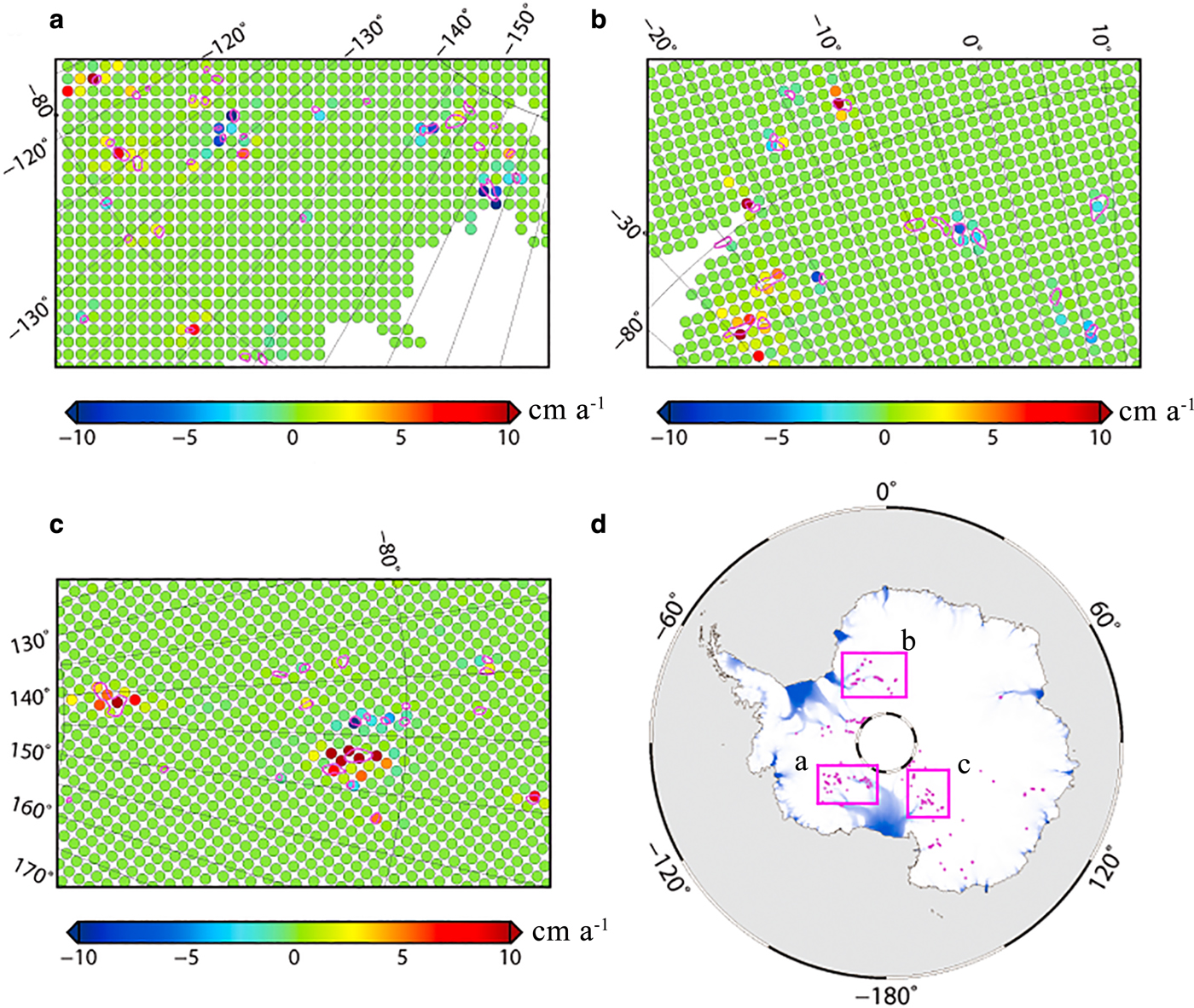
Fig. 6. The difference between the combined GIA rates before and after the elimination of observations above subglacial lakes in the region of (a) Slessor Glacier and Recovery Glacier, (b) Kamb Ice Stream and Scott Glacier, and (c) Byrd Glacier and Nimrod Glacier. In a, b and c, purple outlines represent boundaries of ASLs. Color-coded dots by the colour bar represent the grid points with a spatial resolution of 20 km × 20 km as the ICESat surface height change rates mentioned in Section 2.1. (d) Locations for 124 ASLs under the AIS, shown as purple points. Background shading shows ice velocities (Rignot and others, Reference Rignot, Mouginot and Scheuchl2011). The red square labelled a, b and c indicate the regions shown in a, b and c, respectively.
4.2. Estimations of present-day GIA over the AIS
The final combined GIA estimates are shown in Figure 7. GIA uplifts in the APIS, the WAIS, Dronning Maud Land, Wilkes Land and the peripheral region of the Filchner-Ronne Ice Shelf, the Ross Ice Shelf and the Amery Ice Shelf. And the highest uplift rates are found in the ASE. Subsidence mostly occurs in Adelie Terre and the East Antarctica inland. As listed in Table 1, in this study, the total GIA-related mass change estimates for the entire AIS, WAIS, EAIS and APIS are 43 ± 38, 53 ± 24, −23 ± 29 and 13 ± 6 Gt a−1, respectively. Uncertainties are 1-σ.
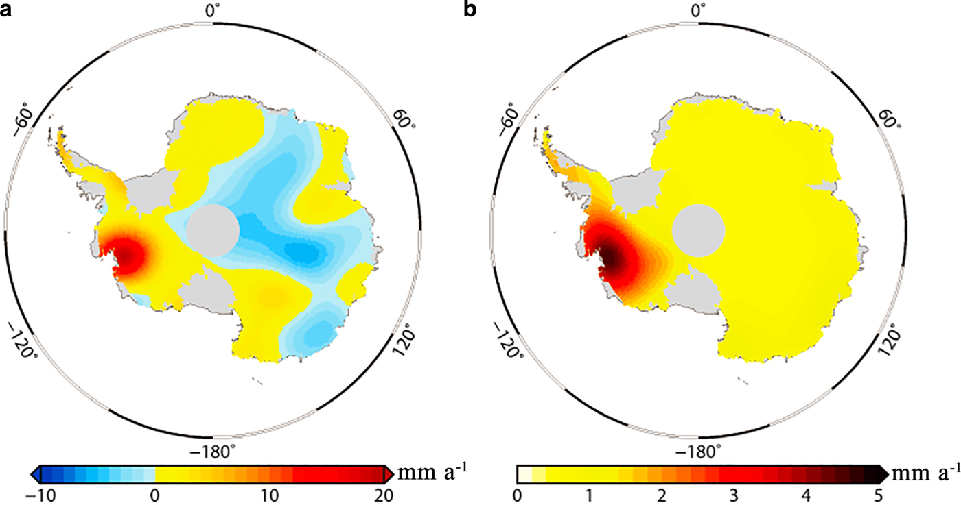
Fig. 7. (a) Estimates and (b) uncertainties for the GIA rates derived from the approach mentioned in Section 3.
Table 1. Estimates of GIA-related mass change and ice mass change from October 2003 to October 2009
Notes: The division of the Antarctic Ice Sheet (AIS) into the Antarctic Peninsula Ice Sheet (APIS), East Antarctica Ice Sheet (EAIS) and West Antarctica Ice Sheet (WAIS) is based on the recent Ice Sheet Mass Balance Inter-comparison Exercise (Shepherd and others, Reference Shepherd2012), and the region of the Amundsen Sea Embayment sector (ASE) is similar to that in Groh and others (Reference Groh2012). ICE-5G, ICE-6G_C, Geruo13, Paulson07 and W12a are GIA models. Their uncertainties are not provided, so the uncertainties of the results derived from those models are not given in this study. Riva09, Gunter12a, Gunter14b and Groh12 are combined results derived by a similar single step combination approach. Gunter14a and Gunter14b are results computed using CSR RL05 regularized and DMT-1b GRACE solutions by Gunter and others (Reference Gunter2014), respectively. Present study is the combined results derived by the iterative method. The results of Riva09, Gunter14a and Gunter14b are quoted from Gunter and others (Reference Gunter2014) because we have not obtained these results. The results of Groh12 are quoted from Groh and others (Reference Groh2012). Groh and others (Reference Groh2012) focus only on a mean GIA rate over the ASE. Uncertainty for the AIS is computed by taking the square root of the sum of squares of the EAIS, WAIS and APIS uncertainties in this study. Uncertainties are 1 − σ.
To assess the performance of our GIA estimates, they are compared with the GIA rates from 5 GIA models, ICE-5G (Peltier, Reference Peltier2004), ICE-6G_C (Argus and others, Reference Argus, Peltier, Drummond and Moore2014), Geruo13 (Geruo and others, Reference Geruo, Wahr and Zhong2013), Paulson07 (Paulson and others, Reference Paulson, Zhong and Wahr2007) and W12a (Whitehouse and others, Reference Whitehouse, Bentley, Milne, King and Thomas2012), and 4 combined GIA rates, Riva09 (Riva and others, Reference Riva2009), Groh12 (Groh and others, Reference Groh2012), Gunter14a and Gunter14b (Gunter and others, Reference Gunter2014). Estimates of GIA-related mass change from these GIA rates are listed in Table 1. The geographical variations of Riva09, Gunter14a and Gunter14b are shown in Figure 8. The geographical variations of ICE-5G, W12a and ICE-6G_C are shown in Figure 9. Because Geuro13 and Paulson07 are both developed using the ICE-5G (VM2) ice model, the results are not shown.
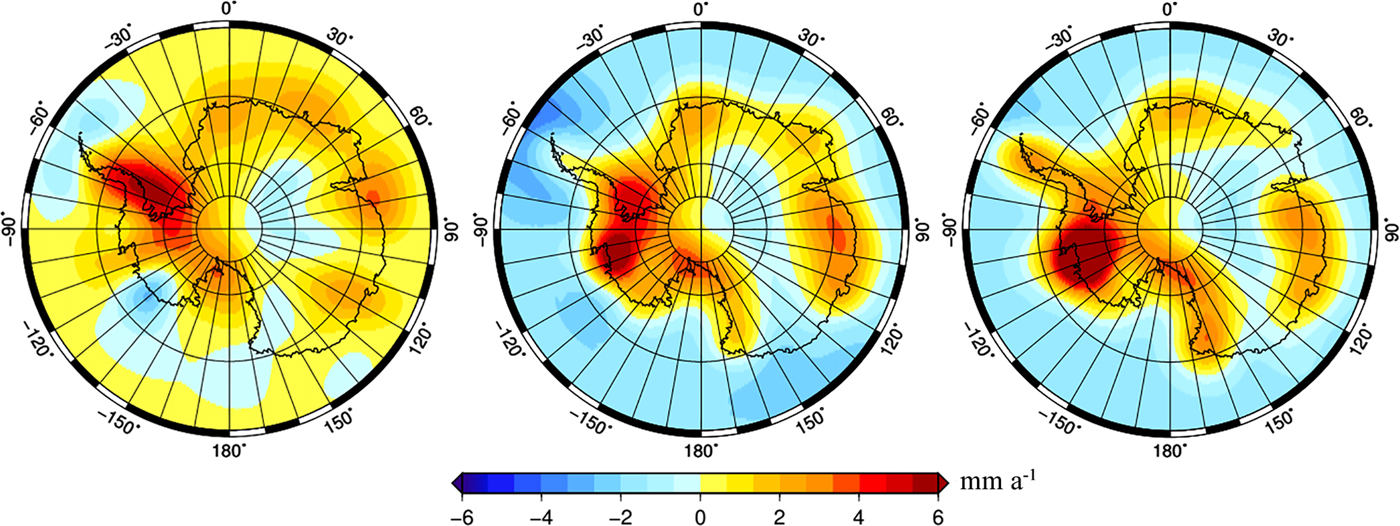
Fig. 8. GIA rates derived from the combined datasets (a) Riva09, (b) Gunter14a and (c) Gunter14b. These three are quoted from Gunter and others (Reference Gunter2014) because we have not obtained the results from Riva and others (Reference Riva2009) and Gunter and others (Reference Gunter2014).
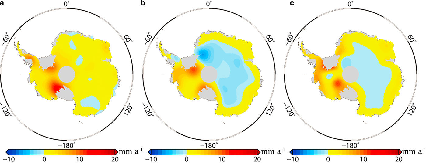
Fig. 9. GIA rates predicted using different GIA models: (a) ICE-5G, (b) W12a and (c) ICE-6G_C.
By comparing Figure 8 with Figure 7a, we find that Gunter14a and Gunter14b show a similar spatial pattern to the GIA estimates presented in this study, whereas Riva09 shows a significant difference in the degree of uplift in the ASE from them. This difference is because firn compaction and surface processes are considered by Gunter and others (Reference Gunter2014) and in this study, whereas Riva09 does not take them into account. Gunter14a or Gunter14b are both combined GIA rates calculated by Gunter and others (Reference Gunter2014). The difference between them is that they use different GRACE mass change rates. Gunter14a use the GRACE mass change rates derived from CSR RL05 regularized GRACE solutions, while Gunter14b use the GRACE mass change rates derived from Delft Mass Transport (DMT-1b) models. Even though similar techniques and datasets are employed, several differences still can be found between Gunter14a or Gunter14b and the GIA estimates presented in this study. The obvious differences are that our GIA results have a broader area and a greater degree of subsidence in the EAIS and a broader area and a greater degree of uplift in the ASE than Gunter14a or Gunter14b. These differences may mainly be caused by two factors. One is because Gunter and others (Reference Gunter2014) remove the LPZ GIA bias correction, which is the mean value of the combined GIA rates over the LPZ, from the combined GIA values uniformly. In contrast, the solutions of this study indicate sizeable subsidence in the LPZ. This removal operation could cause Gunter14a and Gunter14b to have a narrower area and a slighter degree of subsidence than the GIA estimates presented in this study. This can also explain why differences in the GIA-related mass change over the EAIS exist between the present study and Gunter14a or Gunter14b, as listed in Table 1. The other factor is that scaling factors are multiplied by GRACE estimates to restore the amplitude dampening caused by truncation, destriping and smoothing in this study, whereas Gunter and others (Reference Gunter2014) do nothing to restore the amplitude dampening. Naturally, gridded GRACE mass change rates derived by Gunter and others (Reference Gunter2014) may underestimate mass loss in the ASE. The undervalued mass change rates would be interpreted as an undervalued GIA uplift in the combination result. It is noted that Gunter14b has a broader area and a greater degree of uplift in the ASE than Gunter14a. This finding provides additional evidence that Gunter14a underestimates the uplifts in the ASE because amplitude dampening is not restored. DMT-1b adopts the anisotropic filtering method developed by Klees and others (Reference Klees2008) to estimate the gridded GRACE mass change rates (Liu and others, Reference Liu2010). Compared with the filtering method used for CSR RL05 regularized GRACE solutions, the anisotropic filtering method developed by Klees and others (Reference Klees2008) can preserve the highest amount of gravity signal while simultaneously minimizing leakage effects and producing smooth solutions in areas of low signal (Klees and others, Reference Klees2008). In other words, the anisotropic filtering method can effectively prevent the underestimation of mass loss in the ASE.Groh12 is an average estimate of the GIA for the ASE. When Groh12 is calculated, leakage effects caused by truncation, destriping and smoothing are reduced using the region function and Lagrange multiplier method (Groh and others, Reference Groh2012). That is, the amplitude dampening is restored. The total GIA-related mass change over the ASE from Groh12 is 34 ± 12 Gt a−1, slightly larger than that from our results, 30 ± 9 Gt a−1, as listed in Table 1. Naturally, it would be larger than that from Gunter12a.
Figure 9 shows the spatial distribution of the predicted GIA rates and three GIA model results with significantly different predictions. Table 1 compares the predictions of GIA-related mass change and ice mass change using more GIA models, including ICE-5G, Geruo13 and Paulson07, as well as W12a, and ICE-6G_C. The predictions derived with ICE-5G, Geruo13 and Paulson07 are different, even though the same ice model is employed. The differences may be attributed to the ice-load history, differing methods of computation and earth model parameters (Groh and others, Reference Groh2012). Given these reason, it can be expected that differences will exist between our GIA estimates and those derived from GIA models. Comparing Figure 9 with Figure 7a, the spatial distribution and the changing magnitude of the GIA rates predicted using the ICE-5G model and our approach are significantly different. Even though the predictions derived with the ICE-6G_C and W12a models have a similar spatial distribution as that of our approach, the uplift over the WAIS and subsidence in the EAIS interior have noticeable discrepancies. Those may be because that GIA models do not consider changes in the ice load that have occurred over the last 1000 years, even though the recent ice load changes have a significant impact on GIA rates (Nield and others, Reference Nield, Whitehouse, King, Clarke and Bentley2012).
4.3. Estimations of ice mass change and the corresponding elastic vertical crustal deformation over the AIS
Estimates and uncertainties for ice mass change rates over the AIS from October 2003 to October 2009 are shown in Figure 10. The spatial pattern of ice mass change rates (Fig. 10a) reveals that the largest ice mass loss signals are concentrated in the northern APIS and ASE, at rates in excess of 10 cm w.e. a−1. Increasing mass gains have occurred in the entire WAIS, except for the regions in Victoria/Oates land and Totten Glacier. Figure 10b shows that larger uncertainties appear in the APIS and ASE, where the mass loss is most significant, and the largest uncertainties are concentrated in the northern APIS. This occurs partly because of the large uncertainties of IMAU-FDM and SMB over these regions. The principal reason is the large uncertainties caused by sparse ICESat observations over these regions and the low resolution of GRACE. Over the ASE and northern APIS, the relatively sparse ICESat measurements in the coastal areas may not sample the fast surface changes sufficiently. Due to the low resolution of GRACE, the dramatic ice mass loss signal in the coastal areas will leak into the ocean. Currently, there is no method that can be used to correct this leakage signal completely. Therefore, the leakage signal may cause large uncertainty in estimations of ice mass change rates, especially in the northern APIS because it is only ~100 km wide, much smaller than the resolution of GRACE.
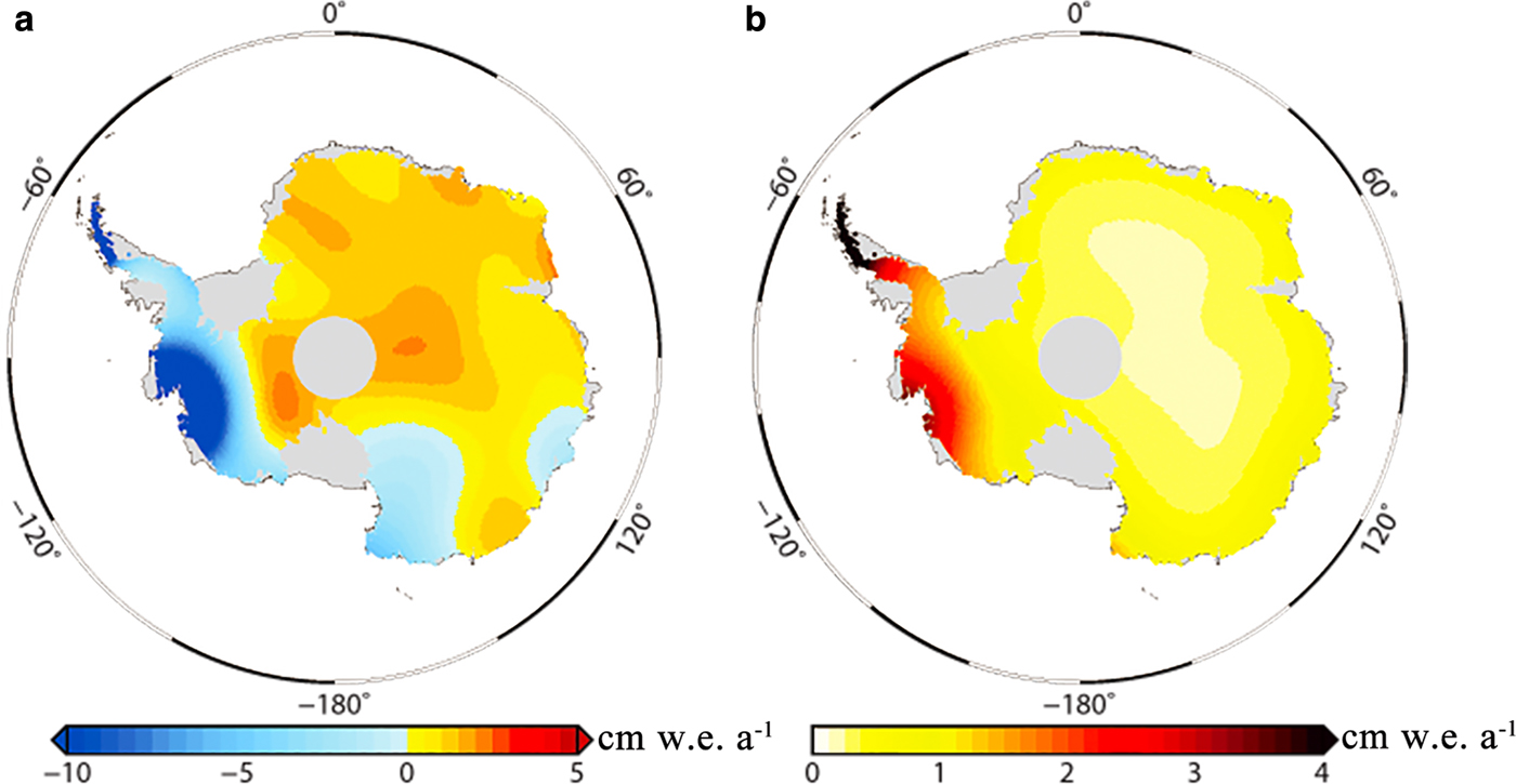
Fig. 10. (a) Estimates and (b) uncertainties for ice mass change rates from October 2003 to October 2009.
Figure 11 shows estimates and uncertainties for elastic vertical crustal deformation rates over the AIS corresponding to ice mass change rates from October 2003 to October 2009. By comparing Figure 11a with Figure 10a, we find that the elastic vertical crustal deformation rates (Fig. 11a) are closely related to the contemporary ice mass change rates (Fig. 10a). The local maxima of elastic vertical crustal deformation rates are in excess of 4 mm a−1 in the ASE and 1.5 mm a−1 in the northern Antarctica peninsula, where the most significant ice mass loss is found. These results agree with those derived from the GRACE data from January 2003 to February 2013 by Argus and others (Reference Argus, Peltier, Drummond and Moore2014), in which the local maxima are 6 mm a−1 near Pine Island Bay and 2 mm a−1 near the tip of the Antarctica Peninsula. The uplift rates of the present study in the ASE are slight smaller than that obtained by Argus and others (Reference Argus, Peltier, Drummond and Moore2014) because of the sudden increase in mass loss rates in 2008, as mentioned above. It should be noted that due to the Gaussian filter used in the calculation, the results of the elastic vertical crustal deformation rates are characterized by lower resolutions and smaller amplitudes than the genuine signal. Figure 11b shows the regions of higher uncertainties also located in the APIS and ASE, correlating to regions of highest uncertainty in the ICESat, IMAU-FDM and SMB datasets.
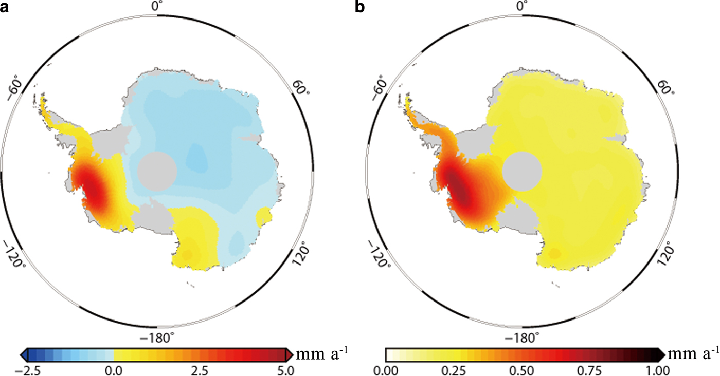
Fig. 11. (a) Estimates and (b) uncertainties for elastic vertical crustal deformation rates corresponding to ice mass change rates from October 2003 to October 2009.
Regarding the total ice mass change estimates from October 2003 to October 2009, the values are listed in Table 1. The present study infers that the total ice mass loss rate estimated is −46 ± 43 Gt a−1 for the entire AIS from October 2003 to October 2009, including −20 ± 6 Gt a−1 for the APIS, −104 ± 25 Gt a−1 for the WAIS and 77 ± 35 Gt a−1 for the EAIS. The total ice mass loss rate over the AIS obtained in Gunter and others (Reference Gunter2014) is −100 ± 44 Gt a−1 (Gunter14a, Gunter14b), which is much higher than the prediction of the present approach. It should be noted that the difference of ice mass changes over the WAIS derived with Gunter14a and our approach is negligible, with an amount of 1 ~ 2 Gt a−1, although the predictions of GIA-related mass change derived with Gunter14a and our approach have a difference of 26 Gt a−1. We consider the difference to be due to the fact that the ice mass change estimated by Gunter and others (Reference Gunter2014) includes the mass change of the integration zone at 400 km extended off the coastline. They add the ice mass change signal back, which leaks into the ocean due to truncation, destriping and smoothing, and reduce the underestimation of ice mass loss caused by the underestimated GIA uplift rates in the WAIS. However, including the mass change of the integration zone at 400 km extended off the coastline in the total mass change may overestimate the ice mass loss. According to Mitrovica and others (Reference Mitrovica, Tamisiea, Davis and Milne2001), water migrates away from the ice sheet because of reduced gravitational attraction resulting from ice-sheet mass loss. The water migrating away was included in the total ice mass by them, resulting in the overestimation of the ice mass loss.
A comparison with the results derived from GRACE data with GIA models shows that, regardless of significant differences in the spatial distribution, the total ice mass loss rates over the entire AIS estimated using W12a (−24 Gt a−1) and ICE-6G_C (−64 Gt a−1) are close to our estimation (−46 ± 43 Gt a−1), whereas those estimated using ICE-5G, Geruo13 and Paulson07 are much larger than our estimations. Meanwhile, our result for the entire AIS is in agreement with the results of the Ice Sheet Mass Balance Inter-comparison Exercise (IMBIE) study (Shepherd and others, Reference Shepherd2012) from GRACE data using the IJ05_R2 and W12a models (−81 ± 33 Gt a−1 from January 2003 to December 2010 and −57 ± 50 Gt a−1 from October 2003 to December 2008) but smaller than that using the ICE-5G model (−160 ± 34 Gt a−1 from January 2003 to December 2010 and −137 ± 49 Gt a−1 from October 2003 to December 2008). In general, the ice mass change uncertainties match those of the IMBIE study, as well as Gunter and others (Reference Gunter2014) study.
5. CONCLUSIONS
Based on previous studies (Wahr and others, Reference Wahr, Wingham and Bentley2000; Velicogna and Wahr, Reference Velicogna and Wahr2002; Riva and others, Reference Riva2009; Groh and others, Reference Groh2012; Gunter and others, Reference Gunter2014), a new iterative method is used to simultaneously estimate the present-day GIA, ice mass change and corresponding elastic vertical crustal deformation over the AIS by combing GRACE and ICESat datasets with the firn compaction and surface processes accounted for by incorporating a firn densification model in the spatial domain constrained by GPS vertical crustal deformation rates.
From this study, GIA uplift rates are found in the APIS, the WAIS and Dronning Maud Land, and subsidence rates mostly occur in Adelie Terre and the East Antarctica inland. The total GIA-related mass change over the entire AIS is 43 ± 38 Gt a−1 (WAIS: 53 ± 24 Gt a−1, EAIS: −23 ± 29 Gt a−1, APIS: 13 ± 6 Gt a−1). From October 2003 to October 2009, the ice mass change for the entire AIS is −46 ± 43 Gt a−1 (WAIS: −104 ± 25, EAIS: 77 ± 35, APIS: −20 ± 6). The largest ice mass loss signals are concentrated in the northern APIS and ASE, at rates in excess of 10 cm w.e. a−1, and increasing mass gains occur in the entire WAIS, except for the regions in Victoria/Oates land and Totten Glacier. For the corresponding elastic vertical crustal deformation rates, the maximum uplifts were concentrated in the Amundsen Sea sector, at more than 4.5 mm a−1, and the second highest uplifts were concentrated in the Northern Antarctic Peninsula, at ~2 mm a−1.
Though the effects of ASLs, on the magnitude of 1 mm a−1, have been considered to improve the accuracy of the combined results, some other issues have not yet been resolved. The main issues are the strategy of constraining the combined results by GPS and the limited spatial resolution and signal leakage of GRACE. Though there are more than 60 GPS sites across Antarctica, they are still sparse considering the vast AIS. In addition, they are spaced very unevenly across Antarctica, especially in the interior of the Antarctic ice sheet, with over 1000 km intervals between sites. Because GPS stations are in shortage in this region, the corrections may be of lower accuracy. Therefore, in this region, additional data and a creative strategy for constraining the combined results, such as that proposed in this study, are needed. The other issue comes from the limited resolution of GRACE. In the narrow zone, such as the northern APIS, because the geographical extent of this region (only ~100 km wide) is smaller than the resolution of GRACE (~200 km at best), mass change rates derived from GRACE will include large uncertainty. Another issue regarding mass change rates obtained from GRACE data is signal leakage. Dramatic ice mass loss signals in the coastal areas will leak into the ocean. However, to this day, there is no way to completely correct this leakage signal. Therefore, the leakage signal may cause large uncertainty in estimations of ice mass change rates.
ACKNOWLEDGEMENTS
We thank Ligtenberg, S.R.M for providing the FDM and SMB, Peltier W. R. for providing the ICE-5G and ICE-6G_C, Whitehouse P. for providing the W12a, Geruo A. for providing the Geruo13 and Paulson A. for providing the Paulson07. The ICESat data were provided by the National Snow and Ice Data Center (NSIDC), and the CSR GRACE solutions were obtained from the Physical Oceanography Distributed Active Archive Center (PO.DAAC) at the NASA Jet Propulsion Laboratory, Pasadena, CA. All geographical plots were produced using the Generic Mapping Tools (GMT). This study is funded by the Key Program of National Natural Science Foundation of China (41531069), the Chinese Polar Environment Comprehensive Investigation and Assessment Programs (CHINARE2016-02-02) and the National Key Research Development Program of China (2016YFB0502204). Editor Hamish Pritchard, Lynsey Rowland and two anonymous reviewers are thanked for their comments that helped clarify and improve the manuscript.
AUTHOR CONTRIBUTION STATEMENT
Baojun ZHANG performed all calculations and wrote most of the manuscript, Zemin WANG and Fei LI proposed the research topic and designed research project, Jiachun AN analysed results and helped in writing the manuscript, Yuande YANG helped in calculating the GRACE and ICESat data, Jingbin LIU revised the manuscript.


 Open access