

Introduction
An ice crystal is highly anisotropic in its response to stress. An ice sheet is made up of an unfathomably large number of ice crystals oriented in a variety of directions (fabric) and of a variety of shapes and sizes (texture). Only when crystal orientations are uniformly distributed in space can the anisotropic behavior of each individual crystal be ignored – giving rise to isotropic behavior in response to stress. However, ice with a preferred orientation of ice crystals (fabric) will behave anisotropically in response to stress. Reference GlenGlen (1955) assumed isotropic behavior in his flow law that has gained wide acceptance in glaciology, as it successfully explained early field observations. Modern field measurements have shown some discrepancies with flow predicted by Glen’s flow law, many of which can be attributed to the fabric in the ice sheet (e.g. Reference Thorsteinsson, Waddington, Taylor, Alley and BlankenshipThorsteinsson and others, 1999).
Paleoclimate reconstruction requires an understanding of flow history in order to relate the depth of the ice (containing the climate proxy) to its age. Changes in flow due to microstructure, such as enhanced strain from fabric or impurity-enhanced ice flow (Reference PatersonPaterson, 1991; Reference Faria, Kipfstuhl, Azuma, Freitag, Weikusat, Murshed and KuhsFaria and others, 2009), need to be accounted for in the ice-flow models used in paleoclimate reconstruction. Flow disturbances can also reorder the layers of ice, altering the depth– age relation. This reordering can happen at any scale, and microstructural observations provide insights into the integrity of ice-core stratigraphy such as ice-core line-scanners (Reference SvenssonSvensson and others, 2005; Reference Faria, Freitag and KipfstuhlFaria and others, 2010), optical and electron microscopy and X-ray diffraction and tomography (Reference Faria, Freitag and KipfstuhlFaria and others, 2010). Further, microstructural changes often coincide with changes in ice chemistry. Ice with high numbers of grain boundaries, triple junctions and micro-inclusions may smear the signal for entrapped gases and dissolved ions (Reference Faria, Freitag and KipfstuhlFaria and others, 2010). Detailed microstructural studies are needed for paleoclimate reconstruction to ensure the integrity of the depth–age relation, ice-core strata and the climate proxies. Microstructure itself, however, has not yet been able to reconstruct a record of past climate changes (it is not a climate proxy).
From the detailed microstructure studies that have been carried out in ice cores for both Antarctic and Greenlandic ice, it is well accepted that ice often develops a preferred crystal orientation (e.g. Reference PatersonPaterson, 1991; Reference Arnaud, Weiss, Gay and DuvalArnaud and others, 2000; Reference Di Prinzio, Wilen, Alley, Fitzpatrick, Spencer and GowDi Prinzio and others, 2005; Reference DurandDurand and others, 2007; Reference Gow and MeeseGow and Meese, 2007). Near ice divides, the pattern of crystal orientations, or fabric, is commonly a vertically oriented single-maximum or vertical-girdle fabric. The strength of the fabric typically increases through the depth of an ice sheet. The profile of fabric with depth at a particular site, however, depends on temperature and strain history. Reference PatersonPaterson (1991) showed that Ice Age ice typically has a smaller crystal size and stronger fabric than Holocene ice, providing the first hint of a connection between paleoclimate and microstructure. A recent sonic velocity profile of Dome C, East Antarctica, has shown transitions in the fabric that correlate to glacial–interglacial transitions through the depth of the ice sheet (Reference Gusmeroli, Pettit, Kennedy and RitzGusmeroli and others, 2012). Furthermore, Reference PettitPettit and others (2011) showed a strong correlation between δ 18O, a known climate proxy, and fabric data, implying fabric records climate information. Therefore, fabric may become a climate proxy in the future.
The variable growth of snow crystals in the atmosphere is unlikely to be preserved in the snowpack, even though snow-crystal growth is highly dependent on the climate in which it is growing (Reference Kobayashi and OuraKobayashi, 1967). Once deposited, the crystals break to a small average size (<1 mm2; Reference BensonBenson, 1962) with nearly random orientations, such that their size and orientation do not directly record atmospheric temperature (Reference HookeHooke, 2005). After landing, snow crystals begin to grow and change shape immediately, due to temperature and vapor-pressure gradients in the firn (Reference ColbeckColbeck, 1983), and it is here that we expect the climate signal to be imprinted into the ice (Reference Carns, Waddington, Pettit and WarrenCarns and others, 2010).
In polar regions, vapor deposition is the primary method of crystal growth in the upper firn. The deposition of vapor on a crystal face is anisotropic: deposition will favor either the basal or prism faces of the snow crystal, depending on the temperature (Reference Nelson and KnightNelson and Knight, 1998). This process causes crystals with the preferred face parallel to the vapor-pressure gradient to grow more than crystals in a less favorable orientation. These crystals grow at the expense of other crystals; as the average size of the crystals increases, the number of crystals decreases (Reference ColbeckColbeck, 1983). This causes the well-oriented crystals to be more likely to remain, while poorly oriented crystals disappear. Therefore, variations in texture and fabric are primarily due to variations in temperature and vapor-pressure gradient (Reference Carns, Waddington, Pettit and WarrenCarns and others, 2010). Because temperature and vapor-pressure gradients are a function of accumulation rate, air temperature and wind strength, this firn crystal evolution process records the climate signal within the firn column. Observations from firn cores have shown a preferred orientation of crystals in the firn layer (Reference Di Prinzio, Wilen, Alley, Fitzpatrick, Spencer and GowDi Prinzio and others, 2005; Reference Fujita, Okuyama, Hori and HondohFujita and others, 2009, Reference Fujita2012).
Climate variables, including temperature, solar radiation, winds and accumulation rate, are not the only factors that control variations of texture and fabric in the firn. The mechanics of densification may cause crystals to break apart, and rotate as they are compressed. Because the underlying physics in this region is poorly understood and much beyond the scope of this paper, we assume here that these climate variables affect the initial orientation and size of the ice crystals due to changes in the firn air temperature, vapor-pressure gradient and accumulation rate. The magnitude and rate of change of these variables during a climate transition will determine how pronounced the initial fabric variation is.
The aim of this paper is to determine how well climate information, as recorded in the initial fabric, may be preserved throughout the depth of an ice sheet. We model the evolution of a climate-induced fabric variation below the firn–ice transition. The fabric is evolved in response to a stress–time profile in which the stress is either constant or varies in a similar way to a real ice divide. Specifically, our model follows a small block of ice as it travels along a particle path. The block of ice is made up of three layers of 8000 crystals or grains (each grain is considered to be a single crystal, and the terms could be used interchangeably throughout this paper; we will use the term crystal because it is the term most often associated with fabric). The model does not include the larger-scale feedbacks among ice with different rheological properties that may alter the stress history along a particle path. Our goal here is to isolate the effects of crystal-scale processes on the evolution of fabric under uniaxial compression and pure shear.
In the following sections, we show which stress–temperature conditions can lead to a preservation of the fabric variation through tens of thousands of years and deep in the ice-sheet divide. First, we provide a brief background on fabric evolution and the relevant crystal processes. We then describe our model in detail and introduce a new orientation distribution function (ODF) to describe the orientations of crystals. In the remaining sections, we describe and discuss the results of our experiments with both constant applied stresses and stress–time profiles from an ice divide.
Background
The deformation of a single ice crystal in response to stress is strongly anisotropic. Crystals shear easily along the slip systems in their basal planes, much like a deck of cards, while shear on other slip systems is nearly two orders of magnitude harder (Reference Duval, Ashby and AndermanDuval and others, 1983). This leads to crystals responding to applied stress by elongating in the direction of the tensile stress and rotating until its basal planes are perpendicular to the compressive stress (Reference Azuma and HigashiAzuma and Higashi, 1985; Reference AlleyAlley, 1992; Reference Van der Veen and WhillansVan der Veen and Whillans, 1994). In polycrystalline ice (hereafter referred to as ice), the orientation of a crystal is defined by the crystallographic axis (c-axis) that is perpendicular to the basal plane. Ice with a random orientation of c-axes (uniform over the surface of the sphere) is considered isotropic, while ice with a preferred orientation of c-axes is anisotropic. Strongly anisotropic ice in simple shear can deform up to an order of magnitude faster than isotropic ice (Reference AzumaAzuma, 1994; Reference Castelnau, Duval, Lebensohn and CanovaCastelnau and others, 1996; Reference ThorsteinssonThorsteinsson, 2001). Ice at depth in an ice sheet tends to have crystals with c-axes aligned vertically (e.g. Reference AlleyAlley, 1992), so its flow is significantly affected by crystal fabric.
The state of stress in the central regions of an ice sheet is dominated by vertical compression combined with horizontal shear that increases in magnitude with depth and distance from the divide. Under this stress state, the crystals tend to align with basal planes oriented horizontally, and their c-axes oriented vertically, as they move deeper in the ice sheet through time, strengthening the fabric with depth. The rate at which crystals rotate (how quickly fabric evolves) depends primarily on strain rate, which is a function of temperature, impurity content, crystal orientation (Reference Weertman, Whalley, Jones and GoldWeertman, 1973; Reference Budd and JackaBudd and Jacka, 1989; Reference PatersonPaterson, 1991) and neighboring crystal interactions (Reference ThorsteinssonThorsteinsson, 2002).
The evolution of fabric is significantly affected by three additional processes: normal crystal (grain) growth, polygonization and migration recrystallization (Reference AlleyAlley, 1992). In solid ice, normal crystal (grain) growth occurs through migration of crystal boundaries driven by energy differences across the boundary defined by boundary curvature, intrinsic properties (e.g. temperature, thickness, diffusivity of water molecules) and extrinsic material (e.g. impurities, bubbles). Almost every experimental and theoretical treatment of the intrinsic growth rate of an ice crystal describes growth rate by a parabolic growth law (Reference Alley, Perepezko and BentleyAlley and others, 1986). The crystal diameter, D, increases with time as
where K is the crystal-growth factor, t is time, t 0 is the time of the last recrystallization and D 0 is the crystal diameter at time t 0. The crystal-growth factor, K, is
where K
0 is a constant that depends on the intrinsic properties of the crystal boundaries, Q is the thermal activation energy, ![]() is the gas constant and T is the temperature. However, extrinsic materials reduce the rate of boundary migration and can be described by a drag force on the boundary (Reference Alley, Perepezko and BentleyAlley and others, 1986). This drag effectively reduces the crystal-growth factor, K.
is the gas constant and T is the temperature. However, extrinsic materials reduce the rate of boundary migration and can be described by a drag force on the boundary (Reference Alley, Perepezko and BentleyAlley and others, 1986). This drag effectively reduces the crystal-growth factor, K.
Normal crystal growth is active throughout the depth of an ice sheet. Once the ice starts deforming, crystal-boundary migration is a function of strain energy and grain-boundary energy. In the special case of the crystals on either side of the boundary having the same strain energy, Eqn (1) will describe the crystal growth in deforming ice. Even though the crystals continue growing at depth, a stable crystal size is typically reached (below a certain depth) because polygonization counteracts crystal growth. Polygonization creates new crystal boundaries within large ice crystals, effectively dividing the crystal in two. Large crystals can become highly strained and experience differential stress, which is relieved by the organization of dislocations into a sub-crystal boundary (Reference AlleyAlley, 1992). Reference De La Chapelle, Castelnau, Lipenkov and DuvalDe La Chapelle and others (1998) determined that the minimum dislocation density needed to form a sub-crystal boundary is ρ p = 5.4 × 10¹⁰ m−2.
Because polygonization depends upon a minimum dislocation density being reached, the rate of polygonization can be indirectly described through the rate of change of the dislocation density. Dislocation density changes due to two dominant processes: it increases due to work hardening and decreases due to absorption of dislocations at the crystal boundary (Reference Miguel, Vespignani, Zapperi, Weiss and GrassoMiguel and others, 2001). Therefore, the change in the dislocation density can be described as
where the first term on the right-hand side describes work hardening: ![]() is the second invariant of the strain-rate tensor, b is the length of the Burgers vector and D is the crystal diameter (Reference Montagnat and DuvalMontagnat and Duval, 2000). The second term describes the absorption of dislocations at the crystal boundaries: α is a constant and K is the crystal-growth factor.
is the second invariant of the strain-rate tensor, b is the length of the Burgers vector and D is the crystal diameter (Reference Montagnat and DuvalMontagnat and Duval, 2000). The second term describes the absorption of dislocations at the crystal boundaries: α is a constant and K is the crystal-growth factor.
Through most of the depth of an ice sheet, the rate of fabric evolution is a balance between crystal growth, polygonization and crystal rotation. However, migration recrystallization dominates fabric evolution at high temperatures (typically above approximately −10°C; Reference Duval and CastelnauDuval and Castelnau, 1995). Migration recrystallization occurs when the stored strain energy (due to dislocations) in a crystal is greater than the crystal-boundary energy of a new strain-free crystal. The new strain-free crystal is nucleated and rapidly grows at the expense of the old crystal (Reference Duval and CastelnauDuval and Castelnau, 1995). The stored energy due to a dislocation density, E d, can be estimated as
where G is the shear modulus, μ is a constant and R e is the mean average of the dislocation strain field range (Reference ThorsteinssonThorsteinsson, 2002). The energy associated with crystal boundaries, E c, is
where γ g is the energy per area on the boundary (for high-angle boundaries). When E d > E c it is energetically favorable to nucleate a new crystal, which quickly grows to a diameter that scales with the effective stress (e.g. Reference ShimizuShimizu, 1998). The crystal that grows rapidly will form in the most energetically favorable position: about halfway between the compressional and tensional axes, which maximizes the resolved shear stress on the basal planes causing them to deform easily (Reference AlleyAlley, 1992). For uniaxial compression or pure shear, for example, this is 45° from the axis of compression. The grains are initially strain-free, and will have a much lower strain energy than the surrounding grains, allowing them to grow. As the new crystals grow preferentially at orientations favorable for the bulk deformation, the fabric can change significantly; in uniaxial compression, a strong vertical fabric will become a weaker small-circle girdle fabric (Reference Budd and JackaBudd and Jacka, 1989).
The Model
Many models have been proposed to incorporate the effect of fabric into ice-sheet models. Reference Gagliardini, Gillet-Chaulet, Montagnat and HondohGagliardini and others (2009) classify the variety of anisotropic polar ice models into four categories: phenomenological, full-field, homogenization and topological models.
Phenomenological models are large-scale ice-flow models that use a macroscopic formulation of the anisotropy of ice (e.g. Reference MorlandMorland, 2002; Reference Gillet-Chaulet, Gagliardini, Meyssonnier, Montagnat and CastelnauGillet-Chaulet and others, 2005; Reference Placidi, Greve, Seddik and FariaPlacidi and others, 2010). The primary question these models answer is how the anisotropy of ice affects the flow of a glacier or ice sheet. These models are designed for flow studies; computational efficiency is paramount and the anisotropy of ice is parameterized and limited to a few special cases. These models typically represent large areas (m2 to km2) for each representative sample of ice, and fabrics are not passed along flowlines. This entire class of model is unsuitable for our application because we are interested in the evolution of small-scale (cm2 to m2) subtle variations in fabrics as they move along their flowlines.
At the other end of the scale lie the full-field models. These models solve the Stokes equations by decomposing each crystal into many elements, allowing the stress and strain-rate heterogeneity to be inferred at the microscopic scale (e.g. Reference Meyssonnier and PhilipMeyssonnier and Philip, 2000; Reference Lebensohn, Liu and Ponte CastañedaLebensohn and others, 2004). These models are concerned with the microscopic processes within the ice crystal and at the boundaries of the ice crystal. They are generally two-dimensional models and become increasingly computationally difficult as the number of crystals is increased, limiting their application to a small number of crystals. These models are unsuitable for our application because the limited number of crystals does not allow a statistically significant description of fabric on the scale of an ice sheet.
Homogenization models (also called micro–macro models) are used to derive the polycrystalline behavior of the ice from the behavior of single crystals (e.g. Reference LliboutryLliboutry, 1993; Reference Castelnau and DuvalCastelnau and Duval, 1994; Reference Van der Veen and WhillansVan der Veen and Whillans, 1994; Reference GödertGödert, 2003; Reference Gillet-Chaulet, Gagliardini, Meyssonnier, Zwinger and RuokolainenGillet-Chaulet and others, 2006). These models compute the macroscopic (bulk) behavior by averaging over the microscopic (crystal) behavior. Generally these models are primarily focused on the evolution of fabric and describe the fabric as either a discrete or continuous orientation distribution. The topological models (e.g. Reference AzumaAzuma, 1994; Reference ThorsteinssonThorsteinsson, 2002) are a sub-class of the homogenization models that include topological information by taking into account neighbor influences; a crystal surrounded by ‘hard’ crystals will be less likely to deform regardless of its orientation. Reference Sarma and DawsonSarma and Dawson (1996) showed that nearest-neighbor interactions are essential to determining the single-crystal strain given a bulk equivalent strain. Reference ThorsteinssonThorsteinsson’s (2002) model is the only topological model to incorporate crystal growth, rotation and dynamic recrystallization into the fabric evolution. Since the recrystallization process significantly affects the evolution of crystal fabric (Reference AlleyAlley, 1992), we use the model developed by Reference ThorsteinssonThorsteinsson (2001, Reference Thorsteinsson2002) to study the fabric evolution throughout the depth of an ice sheet near a divide. It is important to note that this model is a polycrystal model that solves for fabric evolution and behavior, not a flow model. This model alone will not capture the deformation–fabric feedbacks due to the redistribution of stress (as a result of spatial variations in rheology) within the ice sheet. However, the model could be integrated into an ice-sheet flow model in order to capture this feedback.
The model uses a representative distribution of N individual ice crystals to calculate the bulk response of the ice to stress by averaging over the crystals. The crystals are arranged on a regular cuboidal grid (Fig. 1), where each crystal has six nearest neighbors. The crystals, however, are considered to evolve independently of each other and are embedded in an ice matrix consisting of small crystals, which accommodate the crystal-boundary migration and act as seeds for migration recrystallization (Reference ThorsteinssonThorsteinsson, 2002). Because these crystals are small, they do not contribute significantly to the bulk deformation of the ice. In the case of nearest-neighbor interactions, the crystals are only able to feel that there is a hard or soft crystal nearby and the interaction only affects the crystals’ resolved shear stress (Eqn (10), below). Each layer in the cuboid can be given a sub-distribution of crystals with its own fabric, and the response of each layer to an applied stress can be calculated through time.

Fig. 1. Left: an example of a polycrystalline cuboid with three distinct fabric layers; the top layer is white, the middle layer light gray and the bottom layer dark gray. Each small cube indicates one crystal and each layer has 4 × 4 × 4 = 64 crystals. The three-layered cuboid in our model has 20 × 20 × 20 = 8000 crystals in each layer. Right: an illustration of the crystal packing where each crystal (gray) has six neighboring crystals (white).
Each crystal in the distribution has an associated orientation given by the co-latitude, θ, and azimuth, φ, as well as an associated spherical size of diameter D and dislocation density ρ. The model takes in an initial crystal distribution, stress, and temperature and evolves the crystals through uniform steps in time or strain; Figure 2 outlines the model process. First, the model creates an initial crystal distribution by the method described in the next subsection. The model then applies a stress to the crystal distribution and calculates the individual crystal strain rates and velocity gradients using the analytic flow law developed by Reference ThorsteinssonThorsteinsson (2001, Reference Thorsteinsson2002). Next, it checks the recrystallization conditions (outlined below) and then rotates the crystals. After each time- or strain-step, the model outputs the new distribution of crystals, the bulk strain and the number and type of recrystallization events. This new distribution of crystals is then fed back into the model for the next time-step, along with the new stress and temperature.

Fig. 2. Flow chart of the model. The model is initialized with fabric data, deviatoric stress and temperature. For each time-step, strain rates and velocity gradients are calculated, dynamic recrystallization processes are applied to the fabric and then the crystals are rotated to calculate new fabric data. The new fabric data as well as new stresses and temperatures are fed back into the model to start the next time-step.
In this model, stress is an input; the stress, therefore, must be determined outside the model.
Crystal physics
Ice crystals rotate as a result of the velocity gradient experienced. The velocity gradient is a result of the internal stresses experienced by the ice sheet, and these stresses lie somewhere between two end members: uniform stress and uniform strain rates. Due to the strong crystal anisotropy, the uniform-stress assumption has been shown to be well adapted to describing polycrystalline ice (Reference Castelnau, Duval, Lebensohn and CanovaCastelnau and others, 1996). Therefore, we apply a uniform stress to each crystal in the distribution. We restrict the deformation of the crystal to the basal plane; therefore, the crystal only responds to the components of stress that are in the basal plane (termed the resolved shear stress; RSS). The Schmidt tensor, S, describes the orientation of the crystal, ![]() , relative to the slip directions and has the form
, relative to the slip directions and has the form
where (s) refers to the slip system, ![]() is the direction (Burgers vector) of the slip system and ⊗ is the vector direct (dyadic) product. Then the RSS, τ
(s), on a slip system is
is the direction (Burgers vector) of the slip system and ⊗ is the vector direct (dyadic) product. Then the RSS, τ
(s), on a slip system is
where σ is the deviatoric stress tensor for the stress applied to the fabric and ![]() summing over repeated indexes. The magnitude of the RSS,
summing over repeated indexes. The magnitude of the RSS, ![]() , can then be calculated as
, can then be calculated as

Using the analytic flow law (Reference ThorsteinssonThorsteinsson, 2001, Reference Thorsteinsson2002) the velocity gradient of a crystal, Lc, in response to a stress is

where β is a constant, ![]() is the flow parameter from Glen’s flow law (Reference PatersonPaterson, 1994, p.97),
is the flow parameter from Glen’s flow law (Reference PatersonPaterson, 1994, p.97), ![]() is the local softness parameter due to explicit nearest- neighbor interactions (NNI) of the ice crystals and n is the exponent in Glen’s flow law (Reference GlenGlen, 1955). The local softness parameter averages the magnitude of the RSS over a crystal’s six nearest neighbors relative to the magnitude of the RSS it is experiencing,
is the local softness parameter due to explicit nearest- neighbor interactions (NNI) of the ice crystals and n is the exponent in Glen’s flow law (Reference GlenGlen, 1955). The local softness parameter averages the magnitude of the RSS over a crystal’s six nearest neighbors relative to the magnitude of the RSS it is experiencing, ![]() :
:

where ζ is the relative contribution of the center crystal, ξ is the relative contribution of each neighbor, and i = 0 refers to the center crystal and i = 1, …, 6 refers to each of the six nearest neighbors (Fig. 1). Because the RSS can be zero, there is a specified roof for the maximum value of ‘. Setting [ζ, ξ] to [1, 0] in Eqn (10) is equivalent to the homogeneous-stress assumption, where there is no NNI. Changing the values of [ζ, ξ] modifies the homogeneous-stress (toward the homogeneous strain) assumption by redistributing the stress through explicit NNI. Using the values [6, 1] means the center crystal contributes as much as all the neighbors together, and [1, 1] means the center crystal and all the neighbors contribute equally.
Finally, the strain rate of a single crystal, ![]() , is
, is
where ()T indicates the matrix transpose.
Rotating crystals
In each time-step, the crystals are rotated from an orientation, ![]() , to a new orientation,
, to a new orientation, ![]() . If the surrounding ice is fixed, each crystal rotates as it deforms according to the standard continuum mechanics rotation rate tensor:
. If the surrounding ice is fixed, each crystal rotates as it deforms according to the standard continuum mechanics rotation rate tensor:
where ![]() is the rotation rate of a single crystal and Lc
is the velocity gradient of a crystal in response to stress (Eqn (9)). If the surrounding ice is rotating within the frame of reference, however, the model calculates a relative crystal rotation rate:
is the rotation rate of a single crystal and Lc
is the velocity gradient of a crystal in response to stress (Eqn (9)). If the surrounding ice is rotating within the frame of reference, however, the model calculates a relative crystal rotation rate:
where ![]() is the bulk rotation rate of the modeled ice in response to stress. The bulk rotation rate is
is the bulk rotation rate of the modeled ice in response to stress. The bulk rotation rate is
where L
m is the bulk velocity gradient of the modeled ice (calculating bulk properties is discussed in the next subection) and ![]() is the rotation rate necessary to add to the modeled bulk rotation rate in order to satisfy the boundary conditions. For example, irrotational deformations (e.g. uniaxial compression, pure shear) should have no bulk rotation of the ice
is the rotation rate necessary to add to the modeled bulk rotation rate in order to satisfy the boundary conditions. For example, irrotational deformations (e.g. uniaxial compression, pure shear) should have no bulk rotation of the ice ![]() , making
, making
Therefore, the new orientation of the crystal is
where t is the time-step.
Bulk properties
The bulk properties are calculated by averaging the single-crystal properties and will be influenced more by larger crystals than smaller crystals. We calculate the volume of a crystal from the its diameter, D, and use its volume fraction, f, as a statistical weight for the calculation of the bulk properties (Reference Gagliardini, Durand and WangGagliardini and others, 2004). Any bulk property, Y, of a single-crystal property, Yc, is then

where

Therefore, the modeled bulk velocity gradient is

where N is the number of crystals in the fabric. Likewise, the bulk strain rate is

Crystal processes
The crystals are additionally affected by normal crystal growth and the recrystallization processes of polygonization and migration recrystallization. Normal crystal growth is implemented by growing the diameter of the crystal, D, according to Eqn (1). Though the ice is deforming, we assume that the small crystals that surround the modeled ice crystal have an average strain energy comparable with the modeled crystal, such that the strain energy does not add to the grain-boundary migration rate. The dislocation density of the crystal also grows, according to Eqn (3). The recrystallization processes are outlined below. Once a crystal has undergone a recrystallization event, it will start to evolve again according to Eqns (1) and (3).
Polygonization
We model polygonization using a proxy for differential stress on a crystal (Reference ThorsteinssonThorsteinsson, 2002). Crystals that have a small component of shear stress resolved on to the basal plane (RSS) will likely be experiencing a differential stress from their neighboring crystals which are deforming. If the ratio of the magnitude of the RSS, ![]() , to the second invariant of the applied stress, ||σ||, is less than a given value
, to the second invariant of the applied stress, ||σ||, is less than a given value ![]() and the dislocation density, p, in the crystal sufficient to form a sub-crystal wall (ρ > ρ
p), then the crystal can polygonize. When a crystal polygonizes, the orientation is changed by an angle, Δθ, in a direction that increases the RSS, the crystal size is halved, and the dislocation density is reduced by ρ
p. Polygonization tends to slow the development of fabric, because crystals that are oriented very close to the preferred orientation (small RSS) of the fabric will polygonize preferentially by the selection criteria (weakening the fabric).
and the dislocation density, p, in the crystal sufficient to form a sub-crystal wall (ρ > ρ
p), then the crystal can polygonize. When a crystal polygonizes, the orientation is changed by an angle, Δθ, in a direction that increases the RSS, the crystal size is halved, and the dislocation density is reduced by ρ
p. Polygonization tends to slow the development of fabric, because crystals that are oriented very close to the preferred orientation (small RSS) of the fabric will polygonize preferentially by the selection criteria (weakening the fabric).
Migration recrystallization
We model migration recrystallization by immediately nucleating a new crystal once the dislocation energy, E d, is greater than the boundary energy, E c (Eqns (4) and (5)). The old crystal is replaced with the new ‘strain-free’ crystal, with dislocation density ρ 0 and a diameter that scales with the effective stress, D ∼ (σklσkl /2)−2/3. The rapid crystal-boundary migration is assumed to be fast enough to grow to a diameter D within a single time-step. The ‘strain-free’ crystal is given the ‘softest’ orientation, or orientation with the highest RSS, of a random set of orientations in the applied stress state (Reference ThorsteinssonThorsteinsson, 2002). In uniaxial compression, this is close to the small circle 45° off the compression axis.
Model parameters
Table 1 lists each parameter used, which equation it can be found in and the relevant reference(s).
Table 1. Values of the parameters used in the model

Generating Initial Crystal Distributions
To generate our initial fabrics, we use a finite number of crystals randomly selected from an orientation distribution function (ODF) to represent the ice we are modeling. Each layer of our cuboid (as shown in Fig. 1) can be given a unique ODF and thereby a unique fabric. The layers are then put together to form our initial crystal distribution.
Orientation distribution functions provide a continuous description of the volume fraction of ice crystals in a certain orientation. This reduces to the relative number of ice crystals in an orientation if every crystal has the same volume. Because thin-section measurements from ice cores provide only a limited snapshot of the ODF in situ, a general ODF is needed to describe the variety of fabrics observed in ice sheets.
It is important to remember that ice crystals are axially symmetric; they have no inherent ‘up’ or ‘down’ direction. Therefore, the orientation of a single ice crystal can equally be described by two unit vectors pointing in opposite directions, ![]() and
and ![]() , corresponding to the two points on opposite sides of the unit sphere where the axis passes through. Because of this symmetry, the space of all possible orientations can be reduced to the upper hemisphere of the unit circle. Every axis will have one end pass through a point on the upper hemisphere, while the other end will pass through a corresponding point (reflected through the origin) on the lower hemisphere. Thus an ODF that preserves this axial symmetry can be defined on the upper hemisphere alone (the unit vector space is restricted to the upper hemisphere). Defined as such, the ODF, p, must be normalized, such that the total volume fraction is equal to 1, or
, corresponding to the two points on opposite sides of the unit sphere where the axis passes through. Because of this symmetry, the space of all possible orientations can be reduced to the upper hemisphere of the unit circle. Every axis will have one end pass through a point on the upper hemisphere, while the other end will pass through a corresponding point (reflected through the origin) on the lower hemisphere. Thus an ODF that preserves this axial symmetry can be defined on the upper hemisphere alone (the unit vector space is restricted to the upper hemisphere). Defined as such, the ODF, p, must be normalized, such that the total volume fraction is equal to 1, or

where S/2 is the surface of the upper hemisphere of the unit sphere, S. Alternately, an ODF, P, could be defined over the whole unit sphere (the unit vector space is unrestricted) such that both ends of the axis carry half the probability of finding a crystal in that orientation ![]() . Again P must be normalized, such that the total volume fraction is equal to 1, or
. Again P must be normalized, such that the total volume fraction is equal to 1, or
It is mathematically equivalent to use either a restricted or unrestricted distribution and, thus far, every ODF proposed in the glaciology literature has been a restricted distribution (Reference Gagliardini, Gillet-Chaulet, Montagnat and HondohGagliardini and others, 2009).
We use an unrestricted distribution called the Watson distribution, the simplest well-known axial distribution in directional statistics (Reference Fisher, Lewis and EmbletonFisher and others, 1987; Reference Mardia and JuppMardia and Jupp, 2000). The Watson distribution (Reference WatsonWatson, 1965) is defined over the whole unit sphere as
where k ∊ [−∞, ∞] is the concentration parameter, ![]() is the principal axis of the distribution and ak
is the normalizing constant. If we set
is the principal axis of the distribution and ak
is the normalizing constant. If we set ![]() , the normalizing constant is
, the normalizing constant is

The Watson distribution preserves axial symmetry, ![]() , and is rotationally symmetric around its principal axis,
, and is rotationally symmetric around its principal axis, ![]() . If the principal axis is pointing vertically,
. If the principal axis is pointing vertically, ![]() , the Watson distribution can be written as
, the Watson distribution can be written as
where θ and φ are the co-latitude and azimuth angles.
The Watson distribution describes single-maximum fabrics when k < 0, equatorial-girdle fabrics when k > 0, and reduces to the uniform (isotropic) distribution when k = 0. Fortunately, these are the most common types of fabrics observed in ice cores (Reference PatersonPaterson, 1994). Additionally, if there is a sample of N observations of axis positions, the Watson distribution’s concentration parameter and principal axis can be determined from the eigenvalues and vectors of ![]() , the orientation tensor used to analyze ice-core thin sections (Reference WoodcockWoodcock, 1977; Reference Gagliardini, Durand and WangGagliardini and others, 2004). Therefore, we can connect the concentration parameter and the principal axis of the Watson distribution to an observed fabric (described in the next subsection).
, the orientation tensor used to analyze ice-core thin sections (Reference WoodcockWoodcock, 1977; Reference Gagliardini, Durand and WangGagliardini and others, 2004). Therefore, we can connect the concentration parameter and the principal axis of the Watson distribution to an observed fabric (described in the next subsection).
Although unrestricted distributions have not been used previously in the glaciology literature, the Watson distribution is closely related to the Fisher distribution, the best-known vectorial (not axial) distribution in the field of directional statistics (Reference Fisher, Lewis and EmbletonFisher and others, 1987; Reference Mardia and JuppMardia and Jupp, 2000). Reference LliboutryLliboutry (1993) proposed a restricted form of the Fisher distribution to use as an ODF in glaciology, but abandoned it due to computational difficulties. Later, Reference Gagliardini, Gillet-Chaulet, Montagnat and HondohGagliardini and others (2009) showed that for Dome C, the restricted Fisher distribution best fit the observed distribution of crystals, as compared to the other ODFs used in the glaciology literature, even though it has never been applied in glaciology. The Fisher distribution, ![]() , is defined as
, is defined as
where ![]() is a normalizing constant, κ∊[0, ∞] is the concentration parameter,
is a normalizing constant, κ∊[0, ∞] is the concentration parameter, ![]() is the principal axis of the distribution and
is the principal axis of the distribution and ![]() is a crystal orientation (unit) vector (Reference FisherFisher, 1953). When the principal axis,
is a crystal orientation (unit) vector (Reference FisherFisher, 1953). When the principal axis, ![]() , is vertical, the density of the distribution reduces to exp κ cos(θ)], where θ is the colatitude angle. The Fisher distribution describes single-maximum fabrics when κ. > 0, and reduces to the uniform (isotropic) distribution when κ. = 0. Unfortunately, the Fisher distribution cannot describe girdle fabrics and it is not axially symmetric
, is vertical, the density of the distribution reduces to exp κ cos(θ)], where θ is the colatitude angle. The Fisher distribution describes single-maximum fabrics when κ. > 0, and reduces to the uniform (isotropic) distribution when κ. = 0. Unfortunately, the Fisher distribution cannot describe girdle fabrics and it is not axially symmetric ![]() , so must be used in the restricted unit vector space for ice crystals. Reference WatsonWatson (1982) showed that an axial form of the (unrestricted) Fisher distribution can be created by replacing θ with 2θ, thereby creating a bipolar distribution. By noticing that exp [cos (2θ)] ∝ exp [cos2 (θ)] we arrive back at the Watson distribution, which, by choosing an appropriate k, can be used in place of Lliboutry’s restricted Fisher distribution, with the added benefit of being able to describe girdle fabrics.
, so must be used in the restricted unit vector space for ice crystals. Reference WatsonWatson (1982) showed that an axial form of the (unrestricted) Fisher distribution can be created by replacing θ with 2θ, thereby creating a bipolar distribution. By noticing that exp [cos (2θ)] ∝ exp [cos2 (θ)] we arrive back at the Watson distribution, which, by choosing an appropriate k, can be used in place of Lliboutry’s restricted Fisher distribution, with the added benefit of being able to describe girdle fabrics.
Orientation tensor
The orientation tensor, built from the orientation of each crystal in a polycrystal, is used to determine the strength of the fabric in the ice (Reference WoodcockWoodcock, 1977; Reference Gagliardini, Durand and WangGagliardini and others, 2004). The orientation tensor is calculated from a polycrystal of N crystals as

where fn
is the crystal’s volume fraction (Eqn (18)). The eigenvalues (ei for i = 1, 2, 3) and eigenvectors ![]() are then calculated from A. The eigenvalues are said to describe the spatial strength of the fabric and the eigenvectors form the best material symmetry basis. Alternately, the eigenvalue, ei, can be considered the fractional variance of the distribution along the eigenvector,
are then calculated from A. The eigenvalues are said to describe the spatial strength of the fabric and the eigenvectors form the best material symmetry basis. Alternately, the eigenvalue, ei, can be considered the fractional variance of the distribution along the eigenvector, ![]() . The eigenvalues are arbitrarily sorted, such that e
1 > e
2 > e
3, and
. The eigenvalues are arbitrarily sorted, such that e
1 > e
2 > e
3, and ![]() gives the direction of the ‘strongest’ fabric. An axially symmetric single-maximum distribution will have eigenvalues such that e
1 > e
2 = e
3 and the principal axis will be
gives the direction of the ‘strongest’ fabric. An axially symmetric single-maximum distribution will have eigenvalues such that e
1 > e
2 = e
3 and the principal axis will be ![]() ; the points will all be clustered around
; the points will all be clustered around ![]() (most of the variance is along
(most of the variance is along ![]() ). While an axially symmetric equatorial-girdle distribution will have eigenvalues such that e
1 = e
2 > e
3, the points will be clustered around the equator of a sphere with a pole axis
). While an axially symmetric equatorial-girdle distribution will have eigenvalues such that e
1 = e
2 > e
3, the points will be clustered around the equator of a sphere with a pole axis ![]() (most of the variance is along both
(most of the variance is along both ![]() and
and ![]() ).
).
If our crystals are considered a random sample of a Watson distribution, then the eigenvalues and eigenvectors of the orientation tensor allow us to estimate the concentration parameter, k, of the Watson distribution (Reference WatsonWatson, 1965). Reference Fisher, Lewis and EmbletonFisher and others (1987, p.176) and Reference Mardia and JuppMardia and Jupp (2000, p.202) show that the maximum-likelihood estimate (MLE) of the concentration parameter, k, is the solution of

where u is the same as in Eqn (24); ![]() and z = k for a bipolar distribution and
and z = k for a bipolar distribution and ![]() and z = −k for an equatorial-girdle distribution. Both Reference Fisher, Lewis and EmbletonFisher and others (1987) and Reference Mardia and JuppMardia and Jupp (2000) give methods to reasonably approximate the solution to Eqn (28). Further, we know the principal axis of the distributions will be
and z = −k for an equatorial-girdle distribution. Both Reference Fisher, Lewis and EmbletonFisher and others (1987) and Reference Mardia and JuppMardia and Jupp (2000) give methods to reasonably approximate the solution to Eqn (28). Further, we know the principal axis of the distributions will be

from the eigenvectors of the orientation tensor. The Watson distribution can thus be calculated to have a fabric that is analogous to a thin section’s fabric.
Taking the Watson distribution to be our general ODF has a few distinct advantages over other proposed ODFs. The Watson distribution is inherently axial, like our ice crystals, and it can be generated directly from the observed properties of a thin section. It describes single-maximum, equatorial-girdle and isotropic fabrics, the most commonly observed in ice cores. Further, it is a well-known distribution in directional statistics (Reference Fisher, Lewis and EmbletonFisher and others, 1987; Reference Mardia and JuppMardia and Jupp, 2000). This allows us to use the statistical tools, such as MLE, developed in a variety of disciplines, from nuclear magnetic resonance imaging (Reference Cook, Alexander and ParkerCook and others, 2004) to the movement of robots (Reference Palmer and FaggPalmer and Fagg, 2009), and many others. (See Reference Fisher, Lewis and EmbletonFisher and others (1987) and Reference Mardia and JuppMardia and Jupp (2000) for more information about the statistical tools that have been developed for this and other spherical distributions.)
We generate the initial fabrics for our model through random sampling of the Watson distribution (Reference UlrichUlrich, 1984; Reference Li and WongLi and Wong, 1993; Reference WoodWood, 1994). Each crystal is assumed to have the same crystal size, and therefore the Watson distribution describes the relative fraction of crystals in a particular orientation. We model the distributions on the fabrics observed at Taylor Dome, Antarctica (as described below).
Constant-Stress Experiments
In order to determine whether a subtle variation in fabric could be preserved over time, we model the application of constant stress on a cuboid that has three 8000-crystal layers, where the middle layer is initialized with a different fabric to the top and bottom layers. The initial fabric for the top and bottom layers is generated with a concentration parameter for the Watson distribution of k = −2.0 (e 1 = 0.538) while the middle layer has a concentration parameter of k = −2.4 (e 1 = 0.567). These concentration parameters are chosen to correspond with fabrics at 100 m depth in Taylor Dome (described below). A contoured Schmidt plot of the fabrics is shown in Figure 3. At each time-step, a constant temperature, T, and stress, σ, is applied to the fabric. We chose our temperature to be T = −30°C, the approximate average temperature of the Antarctic ice sheet. This temperature is well below our cutoff temperature for migration recrystallization, which is therefore not active in the results presented here. We apply the stress states of uniaxial compression and pure shear to our fabric. The deviatoric stress tensor for uniaxial compression has the form

and the deviatoric stress tensor for pure shear has the form


Fig. 3. Contoured Schmidt plot of the initial fabrics for both the constant stress and Taylor Dome experiments where the fabrics are contoured at levels of 0, 2Σ, …, 10Σ. Σ is the standard deviation of the density of crystals from the expected density for isotropic ice (Reference KambKamb, 1959). The top two plots are contour plots of the continuous Watson distribution (an infinite number of crystals) with concentration parameters k = −2.0 (left) and k = −2.4 (right). Two random 8000-crystal fabrics were generated from these Watson distributions, as shown in the bottom two plots. The fabric generated from the k = −2.0 and k = −2.4 distributions have eigenvalues of e 1 = 0:538 and e 1 = 0:567, respectively. The concentration parameter of k = −2.4 is consistent with a fabric at 100 m depth in Taylor Dome, and the concentration parameter of k = −2.0 was picked to make a fabric that is slightly more isotropic.
We use σ values 0.1 and 0.4 bar to provide a lower and upper bound on the characteristic deviatoric stresses typically seen in ice sheets (Reference Pettit and WaddingtonPettit and Waddington, 2003). The model calculates a strain rate at a time-step, and then the fabric is evolved for the amount of time required to achieve a strain-step of 0.001, until a total strain of 0.35 is reached. After 0.35 strain, the time-step necessary for a 0.001 strain-step has increased by over two orders of magnitude, due to stress hardening, and preliminary model runs suggest that the separation in eigenvalues between the layers will drop below 0.01 for most of our experiments. The nearest-neighbor interaction parameters (Eqn (10)) were varied for different model runs. Table 2 shows the model set-up for each run.
Table 2. Summary of the run set-up of our constant-stress experiments

Results
Figure 4 shows the evolution of the e 1 eigenvalues, the number of polygonization events and the model time for each strain-step in the uniaxial-compression tests (runs 1–6 in Table 2). A uniaxial-compression stress environment causes an increase in the fabric strength. For the low-stress runs (1, 3 and 5) polygonization is not active initially because the strain rate is too low to generate dislocations faster than they are being destroyed by recovery processes, unlike the high-stress runs (2, 4 and 6). As the crystals grow, however, the absorption of dislocations at crystal boundaries decreases, triggering polygonization events even as the strain rates decrease due to work hardening. The effect of NNI in these experiments is to change the timing and rate of polygonization. Nearset-neighbor interactions distribute stress among crystals, such that they no longer all experience the same effective stress. This modification of the stress distribution tends to cause polygonization events to be evenly distributed in time, rather than tightly clustered at a threshold strain. In each run, when polygonization becomes active, there is a corresponding reduction in the rate of evolution (slope of the middle graph).

Fig. 4. The uniaxial-compression runs, 1–6 (Table 2). The top row shows the low-stress runs and the bottom row the high-stress runs. The left column shows no nearest-neighbor interaction ([ζ, ξ] = [1, 0]; Eqn (10)), the middle column shows mild nearest-neighbor interaction ([ζ, ξ] = [6, 1]) and the right column shows full nearest-neighbor interaction ([ζ, ξ] = [1, 1]). For each run, the top plot shows the number of crystals that recrystallize within each strain-step, as a percentage of the total number of crystals. The middle plot shows the evolution of the largest eigenvalue, e 1, for the middle layer (solid curve) and the top and bottom layer (dashed curve). The bottom plot shows the total model time at each strain-step.
Figure 5 shows the separation between the eigenvalues, e 1, of the middle and top/bottom layers for runs 1–6. In all cases, we see the separation of the eigenvalues reduced over time because, when all other effects are equal, the rotation rate decreases as the fabric strengthens. However, the separation of eigenvalues reduces slowly enough that the fabric variation is measurable up to at least 0.30 bulk strain. This reduction in the eigenvalue separation happens because each layer’s fabric nears its stress-equilibrium state. All three layers will ultimately approach the same equilibrium fabric because they are under the same stress and temperature, and have the same material properties (e.g. impurity content). Polygonization events tend to slow down fabric evolution, which can result in an increase of the separation if the polygonization events dominate the fabric evolution, as seen in the no NNI runs (1 and 2) at high bulk strains. Likewise, in the high-stress NNI runs (2, 4 and 6), polygonization is very active early in the evolution, due to the high strain rates. In these runs, polygonization and strain-induced rotation are close to being balanced, causing the separation to be maintained to higher bulk strains. The weaker fabric will have a higher strain rate, causing it to be slowed down more by the increased number of polygonization events. However, in the low-stress runs with mild and full NNI (3 and 5), the separation at any given bulk strain will be less than in runs without NNI, because the strain-induced rotation dominates the polygonization. The weaker fabric will be able to evolve faster than the stronger fabric, since it is not being slowed by many polygonization events.

Fig. 5. Separation of the largest eigenvalue, e 1, between the top layer and middle layer for the uniaxial-compression runs, 1–6. The top plot shows the low-stress runs, 1, 3 and 5. The bottom plot shows the high-stress runs, 2, 4 and 6. The solid curves indicate runs 7 and 8 with no nearest-neighbor interaction ([ζ, ξ] = [1, 0]; Eqn (10)), the dashed curves indicate runs 9 and 10 with mild nearest-neighbor interaction ([ζ, ξ] = [6, 1]) and the dotted curves indicate runs 11 and 12 with full nearest-neighbor interaction ([ζ, ξ] = [1, 1])
Figure 6 shows the evolution of the e 1 eigenvalues, polygonization events and total strain for the pure-shear tests (runs 7–12 in Table 2). Similar to uniaxial compression, a pure-shear environment causes a strengthening of the fabric. In the low-stress runs (7, 9 and 11), polygonization events happen at a lower bulk strain, due to larger horizontal strain rates than in the uniaxial-compression runs. Similarly, polygonization is much more active for the high-stress pure-shear runs (8, 10 and 12) than for the uniaxial-compression runs, resulting in the weakest fabrics after 0.35 strain among any of our experiments.

Figure 7 shows the separation between the eigenvalues, e 1, of the middle and top/bottom layers for the pure-shear runs (7–12). As in the uniaxial-compression runs, we see the separation of the eigenvalues decrease over time in all cases, yet remain measurable to at least 0.30 bulk strain. In the low-stress runs with NNI (9 and 11), polygonization starts at lower bulk strains, causing the separation to decrease more quickly than for the no NNI run (7). Polygonization is very active in the high-stress runs (8, 10 and 12), causing the separation to be maintained to a higher bulk strain than in any other test. Polygonization dominates the fabric evolution in the no NNI run (8), causing a large increase in the separation of the eigenvalues, that is more pronounced than in the uniaxial-compression runs.

Fig. 7. Separation of the largest eigenvalue, e 1, between the top layer and middle layer for the pure-shear runs, 7–12. The top plot shows the low-stress runs, 7, 9 and 11. The bottom plot shows the high-stress runs, 8, 10 and 12. The solid curves indicate runs 7 and 8 with no nearest-neighbor interaction ([ζ, ξ] = [1, 0]; Eqn (10)), the dashed curves indicate runs 9 and 10 with mild nearest-neighbor interaction ([ζ, ξ] = [6,1]) and the dotted curves indicate runs 11 and 12 with full nearest-neighbor interaction ([ζ, ξ] = [1,1]).
Taylor Dome Experiments
Taylor Dome is a small peripheral dome (20 km × 8 km) of the East Antarctic ice sheet, just inland of the Transantarctic Mountains, and provides ice to outlet glaciers entering Taylor Valley and McMurdo Sound. An ice core was drilled to bedrock on the summit of Taylor Dome (77° 47′ 47′′ S, 158° 43′26′′ E) to a depth of 554 m in 1994. Near the bed the ice is >230 ka old; the depth–age profile is shown in Figure 8 (Reference SteigSteig and others, 1998, Reference Steig2000). The ‘kink’ in the depth–age profile is synchronous with the last glacial–interglacial transition. The Taylor Dome ice core provides a stratigraphically undisturbed record through the entire last glacial cycle (Reference Grootes, Steig and StuiverGrootes and others, 1994).

Fig. 8. Depth–age profile for Taylor Dome, East Antarctica (Reference SteigSteig and others, 1998, Reference Steig2000).
Ice samples were cut from the ice core for thin-section microstructure analysis. Each thin section’s fabric was determined using an automatic ice fabric analyzer (Reference WilenWilen, 2000; Reference Hansen and WilenHansen and Wilen, 2002; Reference Wilen, Di Prinzio, Alley and AzumaWilen and others, 2003). The instrument consists of an optical bench with two rotating stages containing polarized lenses. A thin section is mounted in a sample holder on the sample stage, between the crossed polarizers. A diffused light source illuminates the sample through one of the polarizers.
The ice fabric analyzer has a digital camera which measures the extinction angle of each pixel from the sample as it is rotated. The sample is rotated nine times in nine different positions. The extinction angle determines the plane containing the c-axis (up to 90°), and the plane intersections from the nine different positions determine the unique c-axis direction. Refraction corrections (analogous to Kamb corrections for manual techniques) are included. An NI LabviewTM routine automatically calculates the angle between the c-axis and the z-axis (θ) and the angle between the projection of c-axis on the x-y plane and the x-axis (φ), for each grain. The error is <0.5° for both θ and φ. This corresponds to a measurement error of less than ±0.001 in the eigenvalues of the thin sections. The fabric profile with depth is shown in Figure 9. The eigenvalues vary by ±0.1 in the top 200 m of Taylor Dome; these variations are two orders of magnitude greater than the measurement error. Because of the low density of thin sections, it is not possible to establish whether these variations are due to climate, statistical fluctuations due to the number of measured crystals, or other microstructural processes. However, these variations are on the order of what we expect from climate variations and, when combined with a higher-density measurement technique (e.g. sonic logging), these are the type of variations that may be preserving a climate signal. Further, the differences in eigenvalues e 2 and e 3 suggest a lack of rotational symmetry; this implies Taylor Dome is not a perfect dome and a combined stress state is required to model it accurately.

Fig. 9. Fabric profile with depth for Taylor Dome. The fabrics were analyzed on an automatic ice fabric analyzer from thin sections of the Taylor Dome ice core. Circles correspond to eigenvalues e 1, squares correspond to eigenvalues e 2 and diamonds to eigenvalues e 3. Measurement errors are less than ±0.001 for the eigenvalues; the error bars are smaller than the data markers in the figure.
Additionally, Taylor Dome has a very low accumulation rate and therefore little advection, leading to a nearly linear temperature profile (Reference Waddington and MorseWaddington and Morse, 1994). We use a linear temperature profile where the temperature, T, at the surface is the mean annual surface air temperature, −43°C, and increases to −26°C at the bedrock (Reference Grootes, Steig and StuiverGrootes and others, 1994; Reference MorseMorse, 1997). As the temperature never gets above −26°C, migration recrystallization activity is likely negligible here; it is well below the theoretical temperature for activation (above approximately −10°C; Reference Duval and CastelnauDuval and Castelnau, 1995).
Experimental set-up
We use the depth–age (Fig. 8) and depth–temperature profiles to model an idealized ice-sheet divide with the characteristics of Taylor Dome. We calculate a depth–stress profile based on an idealized, symmetric ice divide (as described by Reference RaymondRaymond, 1983), defined by the ice thickness and the vertical velocity of ice at the surface. We assume that these profiles are constant through time, so we can use the model time to interpret a depth from the depth–age profile and then stress and temperature from their respective profiles. From these profiles we define a stress–time profile that drives the fabric evolution.
The deviatoric stress components, σij , of a dome-type (circularly symmetric) ice divide are


where ![]() is the flow parameter from Glen’s flow law (Reference GlenGlen, 1955), n is the exponent in Glen’s flow law, v
s is the vertical component of the ice velocity at the surface, h is the ice thickness and d is the depth. We interpret A from the values given by Reference PatersonPaterson (1994, p.97) based on the ice temperature, and v
s from the top of the depth–age profile (the average accumulation rate over the century preceding 1994). Likewise, deviatoric stress components, σij
, of a ridge-type ice divide are
is the flow parameter from Glen’s flow law (Reference GlenGlen, 1955), n is the exponent in Glen’s flow law, v
s is the vertical component of the ice velocity at the surface, h is the ice thickness and d is the depth. We interpret A from the values given by Reference PatersonPaterson (1994, p.97) based on the ice temperature, and v
s from the top of the depth–age profile (the average accumulation rate over the century preceding 1994). Likewise, deviatoric stress components, σij
, of a ridge-type ice divide are

where σ is the same as in Eqn (32).
In reality, Taylor Dome is likely experiencing a higher stress than our idealized model because it assumes a flat bed. It also does not have constant depth–age, depth–temperature and depth–stress profiles. Because our model does not solve for ice flow, the assumptions in our idealized model do not account for possible strain enhancements, such as impurity-enhanced ice flow (Reference PatersonPaterson, 1991; Reference Faria, Kipfstuhl, Azuma, Freitag, Weikusat, Murshed and KuhsFaria and others, 2009), or the feedback between layers with different rheological properties, such as the feedback that can lead to concentrated shearing on layers with crystals oriented to be soft in shear (Reference Budd and JackaBudd and Jacka, 1989; Reference DurandDurand and others, 2007; Reference Pettit, Thorsteinsson, Jacobson and WaddingtonPettit and others, 2007). In general, layers that are rheologically harder in the direction of the dominant stress component will deform more slowly and the fabric will evolve more slowly if surrounded by softer layers; in our model, each layer evolves independently. Therefore, we expect our modeled fabric evolution to be slower and more uniformly distributed between layers than within Taylor Dome.
We calculated a depth–stress profile for both dome-like and ridge-like symmetry, as shown in Figure 10. Taylor Dome falls somewhere between these two end members, but, based on geometry, it is closer to a dome-like symmetry.

Fig. 10. Depth–stress profile for Taylor Dome. The top plot shows a dome-like stress profile and the bottom plot a ridge-like profile. The solid curves correspond to σ 33, the dotted curves correspond to σ 22 and the dashed curves correspond to σ 11.
Similar to our constant-stress experiments, we modeled the evolution of a cuboid with three fabric layers of 8000 crystals. We start the model at a depth just below the pore close-off depth at 100 m, and run the model to a depth 547.2 m through both the ridge-like and dome-like stress profiles. The time-step was 100 years and the modeled depth range corresponds to 210 ka of evolution. For all three layers, we use an initial uniform crystal size, D 0, of 1.5 mm, which is consistent with the average crystal size observed at 100 m depth in Taylor Dome, and agrees with the crystal-growth factor, K, (Eqn (1)) using an initial crystal size of 1 mm (Reference BensonBenson, 1962). For the middle layer, we generated the initial fabric, based on a concentration parameter for the Watson distribution of k = −2.4 (e 1 = 0.567). The concentration parameter was estimated at 100 m depth from a linear interpretation of the thin-section eigenvalues (e 1 = 0.571, e 2 = 0.240 and e 3 = 0.189; Eqn (28)). Since the Watson distribution is circularly symmetric, e 2 and e 3 are set equal to a symmetric distribution with the same vertical concentration; e 2 = e 3 = (1 – e 1 )/2. For the top and bottom layer, we generated fabrics that are slightly less concentrated; k = −2.0 (e 1 = 0.538 and e 2 = e 3 = 0.231). The initial fabrics are shown in Figure 3 (these are the same fabrics as used in the constant-stress experiments). This fabric is evolved for one time-step, and then used as the input for the next time-step. The NNI parameters from Eqn (10) were varied ([ζ, ξ] = [1, 0], [6, 1], [1, 0]) for different model runs (Table 3).
Table 3. Summary of the run set-up of the Taylor Dome experiments
Results
Figure 11 compares the modeled evolution for the middle fabric section of the 100m fabrics for a dome-like stress profile with the measured fabric in Taylor Dome. Likewise, Figure 12 shows the modeled and measured fabric for a ridge-like symmetry. The modeled fabric evolves more slowly than the measured fabric in Taylor Dome because of our model assumptions: the idealized steady-state stress profile we are using and the lack of the fabric–deformation feedback. Nearest-neighbor interactions further slow the evolution of the fabric, because they modify the crystal strain rates (Eqn (10)). This can be seen in the Schmidt plots of the evolved fabrics for each of these cases, which are shown in Figure 13. After the same total strain, the fabric with no NNI has more crystals concentrated towards vertical than the fabric with full NNI (Fig. 14).

Fig. 11. Evolution of fabric within an ice sheet based on Taylor Dome for the dome-like Taylor runs, 13–15 (Table 3). The three left plots show the evolution of the three eigenvalues for the middle fabric layer in Taylor Dome, and the rightmost plot shows the number of polygonization events within a time-step as a percentage of the total number of crystals. In the plots, the gray open circles are thin-section measurements in Taylor Dome, the solid curve corresponds to no nearest-neighbor interaction ([ζ, ξ] = [1, 0]; Eqn (10)), the dotted curve indicates mild nearest-neighbor interaction ([ζ, ξ] = [6, 1]) and the dashed curve indicates full nearest-neighbor interaction ([ζ, ξ] = [1, 1]).


Fig. 13. Contoured Schmidt plots of the evolved middle layer fabric after 2 10 000 years for dome-like (top row) and ridge-like (bottom row) symmetry. The left column shows no nearest-neighbor interaction ([ζ, ξ] = [1, 0]); Eqn (10)), the middle column shows mild nearest-neighbor interaction ([ζ, ξ] = [1, 1]) and the right column shows full nearest-neighbor interaction ([ζ, ξ] = [6, 1]). The plots are contoured in the same way as in Figure 3, but the fabrics are now contoured at levels of 0,20Σ, …, 100Σ.

Fig. 14. The top plot shows the cumulative strain undergone by the modeled fabrics as a function of the largest eigenvalue, e 1, for the dome-like Taylor runs, 13–15 (Table 3) Likewise, the bottom plots show the ridge-like Taylor runs, 16–18. In the plots, the solid curves correspond to no nearest-neighbor interaction ([ζ, ξ] = [1, 0]); Eqn (10)), the dotted curves indicate mild nearest-neighbor interaction ([ζ, ξ] = [6, 1]) and the dashed curves indicate full nearest-neighbor interaction ([ζ, ξ] = [1, 1]).
Figure 15 shows the separation between the largest eigenvalues, e 1, of the middle and top/bottom layers in the dome-like and ridge-like stress tests (runs 13–15 and 16–18, respectively; Table 3) and the number of polygonization events. As in the constant-stress experiments, we see the separation of the eigenvalues decreases over time in all cases, but they remain measurable for 210 ka. In both the dome-like and ridge-like cases, NNI causes the separation to decrease and polygonization starts at lower bulk strains than in the no NNI runs. In the ridge-like runs (16–18) the fabric is adjusting from the circularly symmetric distribution to an elliptical distribution expected from pure shear (Reference PatersonPaterson, 1994). This causes some crystals to have a very high strain rate, causing polygonization to be much more dominant than in the dome-like runs (13–15).
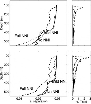
Fig. 15. The top plots show the separation of the largest eigenvalue, e 1, between the top and middle fabric layers for the dome-like Taylor runs, 13–15 (Table 3), as well as the total number of polygonization events within a time-step, as a percentage of the total number of crystals. Likewise, the bottom plots show the ridgelike Taylor runs, 16–18. In the plots, the solid curves correspond to no nearest-neighbor interaction ([ζ, ξ] = [1, 0]); Eqn (10)), the dotted curves indicate mild nearest-neighbor interaction ([ζ, ξ] = [6, 1]) and the dashed curves indicate full nearest-neighbor interaction ([ζ, ξ] = [1, 1]).
Discussion
In all our experiments, a variation in fabric, such as that created by a fluctuation in climate, is preserved until the fabric equilibrates to the stress state. For uniaxial compression and pure shear, there is a ‘window of opportunity’, in which the separation of eigenvalues is sufficient to preserve the climate signal because the weaker fabric takes more time to equilibrate. The minimum separation required to measure a fabric anomaly depends on the measurement technique.
For a constant applied stress, the length of time this window is open depends on the magnitude of the initial fabric variation, the initial strength of the weaker fabric, the magnitude of the applied stress (which controls the strain rate and, therefore, the rate of polygonization) and the strength of the nearest-neighbor interactions. If the fabric variation is small to begin with, it may become immeasurable before either fabric reaches equilibrium. If the fabric variation is sufficiently large, the weaker initial fabric controls the time the window is open because the window closes as this weaker fabric reaches equilibrium with the local stress state (the stronger fabric reaches equilibrium before the weaker fabric). Higher stress leads to higher strain rates and faster rotation of the crystals. Therefore, the fabric will equilibrate and the window will close more quickly in time.
Polygonization plays a major role in the evolution of fabric. Each additional polygonization event rotates a crystal away from the principal stress direction, therefore acting to slow down the strengthening of the fabric. Polygonization events, however, do not occur uniformly in time, because each event requires a threshold dislocation density. At high strain rates (resulting from high stress in our experiments), polygonization events occur often throughout the deformation process. But at the low strain rates we studied, our model predicts a negligible number of polygonization events until 0.20 or 0.30 strain. When neighboring crystals interact, however, polygonization events occur earlier in the deformation process.
Nearest-neighbor interactions minimize the differences in strain rates among neighboring crystals. With NNI, a poorly oriented or hard crystal surrounded by soft crystals will deform faster than without NNI, advancing when the crystal polygonizes. Likewise, a soft crystal surrounded by hard crystals will deform more slowly, delaying when the crystal polygonizes. However, because this crystal is deforming less, it will stay in a softer orientation longer, while the neighboring hard crystals will also move to a softer orientation through polygonizations (their deformation is being increased by the softer crystal). The net effect of this is to increase the overall strain rate of the ice, advance the timing of polygonizations and increase the overall number of polygonization events. Since NNI causes the crystals to bunch up (the hardest crystals get softer and the softest crystals get harder), the window will close more quickly; the separation between the fabrics will be reduced.
By finding the time (and therefore strain) at which the eigenvalues separation is <0.01, we can determine how long the window stays open. Our model results suggest that at low stresses, similar to those found at thick cold ice divides, the window stays open for ∼2000 ka. At higher stresses, similar to those found at smaller ice sheets and ice caps, the window stays open for ∼10 ka.
When we apply this model to Taylor Dome, we see that the low stresses and low temperatures result in maintaining the separation of eigenvalues throughout the depth of the ice sheet. This suggests that a fabric anomaly created by a fluctuation in climate may be measurable deep in the ice: the window stays open. The window stays open even with full NNI implemented. It is important to note that our fabric only evolves to ∼0.30 strain throughout our Taylor Dome profile, since the idealized stress profile was generated with an isotropic ice assumption and our fabric experiences stress hardening as it evolves. Realistically, the fabric would evolve to ∼1.0 strain if the fabric–deformation feedback was included. This may cause the fabric signal to be lost higher up in the ice sheet, however, the fabric–deformation feedback may also cause an initial enhancement of the climate signal by causing the stronger fabric to evolve much faster than the weaker fabric. Integrating this model into a flow model will allow this feedback to be studied.
Conclusions
Our model for fabric evolution in ice suggests that for compressive-stress regimes, total strains of at least 0.30 are necessary to rid fabric of its ‘memory’ of past fabric and stress states. Near an ice divide, most ice does not reach 0.30 total strain until deep in the ice (deeper for cold or low-stress divides, and shallower for warm or high-stress divides). Therefore, we can preserve a fabric anomaly, such as may be induced in the firn by a fluctuation in climate, throughout most of the depth of the ice sheet.
The rate of fabric evolution depends on strain rate, and our model assumes the strain rate is related to stress, based on the analytic flow law developed by Reference ThorsteinssonThorsteinsson (2001, Reference Thorsteinsson2002), which is an extension of Glen’s flow law and uses the typical softness parameters as reviewed by Reference PatersonPaterson (1994, p. 97). As discussed by Paterson, many ways have been suggested to alter the isotropic softness parameter. If we increase the value of the softness parameter in our model, then the same stress will result in higher strain rates. While higher strain rates will rotate the crystals more quickly and increase the rate of fabric evolution, higher strain rates also induce polygonization events, which slows bulk fabric evolution and preserves the fabric anomaly for longer. The net effect of softer ice depends on the balance of these two processes.
If different layers have different isotropic rheologies (e.g. due to differences in impurities), then the complex feedbacks between stress and strain rates may cause the softer ice to have a higher strain rate. This high strain rate will lead to faster fabric evolution unless it triggers polygonization events, which slows down fabric evolution. The fabric evolution will be determined by the balance of these two processes. Furthermore, impurities tend to impede crystal growth, which increases the likelihood of a polygonization event (as Eqn (3) shows, the rate of polygonization is inversely proportional to crystal size).
Differences in rheologies between layers may also be generated by the fabric itself, because, in compression, crystals tend to rotate to a ‘hard’ orientation. The stronger the fabric, the harder the ice in compression. In our model results, this is what causes the decrease in strain rate as the fabric strengthens, slowing the rate of fabric evolution.
Finally, our model assumes cold ice (−30°C), where migration recrystallization is likely negligible. At higher temperatures, when migration recrystallization is known to be active, new, strain-free crystals grow quickly, polygonization events decrease and fabric weakens because the new crystals grow in a ‘soft’ orientation. The effects of migration recrystallization on fabric evolution or the ability to preserve a fabric anomaly is not fully understood. Data from the EPICA Dome C borehole suggest that fabric variability maintains its correlation with climate variability, despite active migration recrystallization (Reference Gusmeroli, Pettit, Kennedy and RitzGusmeroli and others, 2012). Reference KipfstuhlKipfstuhl and others (2009) have shown that migration recrystallization may be active at much lower temperatures and strain rates.
Because a real ice divide is rarely in steady state, often migrating its position laterally, ice rarely experiences only a pure compressive stress state (uniaxial or pure shear). Along its particle path, an ice particle will experience a combination of compressive and simple-shear regimes that varies throughout the depth. Our results suggest what is possible for pure compressive regimes. When simple shear is included, the results may be significantly different. Our goal in this paper was to isolate the compressive regimes, and further work is required to detail the effect of simple shear on a fabric variation.
We can, however, speculate on the response to simple shear of a fabric variation, similar to the one we have studied here, because many of the same principles apply. The primary difference between compressive and simple-shear states of stress is that fabric in simple shear tends to rotate into a ‘soft’ orientation, with respect to the applied stress, rather than into a ‘hard’ orientation, as happens with compressive regimes. This difference results in ice with strong fabrics having higher strain rates than ice with weaker fabrics under the same applied stress. Because fabric evolution depends on strain rate, the stronger fabric will evolve fabric more quickly than the weaker fabric. Rather than simply slowing the decrease in separation (slowly closing the window), there will be a positive feedback that opens the window wider. This effect is observable in the deepest ice in ice sheets, where shear stress is typically highest; this deep ice exhibits the strongest variations in fabric (Reference Gusmeroli, Pettit, Kennedy and RitzGusmeroli and others, 2012).
It is likely that fabric can be developed as a climate proxy, because a climate-induced variation in fabric can be preserved throughout the depth of an ice sheet. Through the use of geophysical inverse methods, it may be possible to use a fabric-evolution model to invert continuous fabric data (e.g. a sonic velocity profile) for past temperatures. However, there is still much research needed for the fabric proxy to be realized. A fabric-evolution model that includes dynamic recrystallization will need to be coupled to an ice-flow model, and the response of fabric variations across a wide variety of stress states will have to be quantified. Furthermore, the parameterizations used to model the dynamic recrystallization processes need to be robust, and new parameterizations may need to be developed, especially in the case of migration recrystallization (Reference KipfstuhlKipfstuhl and others, 2009).
Acknowledgements
We thank Larry Wilen for allowing us to use the Taylor Dome data. We thank Ed Waddington, Regina Carns, Alessio Gusmeroli, Maurine Montagnat, Catherine Ritz and Paul Duval for enlightening discussions on fabric evolution. We thank Paul Jacobson for the many modeling tips he provided, and Ed Beuler for insightful discussions on statistics. Finally, we thank Scientific Editor Jo Jacka and two anonymous reviewers for their comments which considerably improved the manuscript. The work presented in this paper was supported by the US National Science Foundation (NSF) grants OPP#0948247, OPP#0940650, OPP#0636795 and an NSF GK-12 Fellowship to Joseph H. Kennedy.


