


1. Introduction
As snow falls on the surface of the Antarctic ice sheet (AIS), it compacts into glacial ice, transitioning through an intermediate stage called firn. Firn has a density that ranges between that of settled snow ( $300\,\mathrm{kg\,m}^{-3}$) and glacial ice ( $917\,\mathrm{kg\,m}^{-3}$) depending on the network of interconnected pores which exchange air with the atmosphere (van den Broeke, Reference van den Broeke2008; Buizert, Reference Buizert2013). Firn densification into glacial ice is influenced by several factors, such as overburden stress, temperature, grain size, wind, impurity concentration and water content (Arthern and others, Reference Arthern, Vaughan, Rankin, Mulvaney and Thomas2010; Hörhold and others, Reference Hörhold, Laepple, Freitag, Bigler, Fischer and Kipfstuhl2012; Kingslake and others, Reference Kingslake, Skarbek, Case and McCarthy2022; Baker and Ogunmolasuyi, Reference Baker and Ogunmolasuyi2024). Understanding firn densification is important as it affects several processes in ice sheets. Firstly, given that densification changes in response to climatic factors, it causes uncertainty in ice-sheet elevation and mass-balance estimates (Helsen and others, Reference Helsen2008; Smith and others, Reference Smith2020). Secondly, densification results in the closure of the interconnected network of pores, which when closed off, traps gases in the ice. The age difference between the trapped gases and the ice is important for interpreting ice core records (Alley, Reference Alley2000; Cuffey and Paterson, Reference Cuffey and Paterson2010). Lastly, the pore space within firn columns can serve as storage for meltwater from the warming climate, hence, breaking the link between surface melt, runoff and sea-level rise (Harper and others, Reference Harper, Humphrey, Pfeffer, Brown and Fettweis2012; Forster and others, Reference Forster2013; Meyer and Hewitt, Reference Meyer and Hewitt2017). Consequently, a comprehensive understanding of firn processes is crucial for accurately predicting ice sheet responses to climate change (The Firn Symposium team, 2024).
Firn densification is controlled by microstructural evolution (Anderson and Benson, Reference Anderson and Benson1963; Arnaud and others, Reference Arnaud, Barnola, Duval and Hondoh2000). It occurs in three stages, each characterized by distinct mechanisms. Initially, grain boundary sliding, vapor transport and surface diffusion dominate until reaching a density of  $550\,\mathrm{kg\,m}^{-3}$ (Anderson and Benson, Reference Anderson and Benson1963; Gow, Reference Gow1969; Maeno and Ebinuma, Reference Maeno and Ebinuma1983; Alley, Reference Alley1987). In the second stage, pore space reduction limits vapor diffusion, giving way for sintering processes and recrystallization until a density of $830\,\mathrm{kg\,m}^{-3}$ is attained (Gow, Reference Gow1969; Maeno and Ebinuma, Reference Maeno and Ebinuma1983). The depth at $830\,\mathrm{kg\,m}^{-3}$ is typically denoted the pore close-off depth. Here, air becomes trapped in bubbles, slowing the densification process as the bubbles are compressed and eventually diffuse into the surrounding ice (Salamatin and others, Reference Salamatin, Lipenkov and Duval1997). Finally, bubble shrinkage and compression become dominant until the density of ice ( $917\,\mathrm{kg\,m}^{-3}$) is reached (Bader, Reference Bader1965). Several studies have been aimed at shedding more light on the microstructural processes in firn (Maeno and Ebinuma, Reference Maeno and Ebinuma1983; Freitag and others, Reference Freitag, Wilhelms and Kipfstuhl2004; Kipfstuhl and others, Reference Kipfstuhl2009; Lomonaco and others, Reference Lomonaco, Albert and Baker2011; Burr and others, Reference Burr, Ballot, Lhuissier, Martinerie, Martin and Philip2018; Li and Baker, Reference Li and Baker2021; Ogunmolasuyi and others, Reference Ogunmolasuyi, Murdza and Baker2023). However, a comprehensive understanding of large-scale implications of firn densification requires an integration between the underlying microphysics and modeling. To this end, over four decades of effort has been undertaken to develop firn densification models (Herron and Langway, Reference Herron and Langway1980; Alley, Reference Alley1987; Barnola and others, Reference Barnola, Pimienta, Raynaud and K1991; Arnaud and others, Reference Arnaud, Barnola, Duval and Hondoh2000; Kaspers and others, Reference Kaspers, van de Wal, van den Broeke, Schwander, van Lipzig and Brenninkmeijer2004; Ligtenberg and others, Reference Ligtenberg, Helsen and van den Broeke2011; Meyer and others, Reference Meyer, Keegan, Baker and Hawley2020; Stevens and others, Reference Stevens, Verjans, Lundin, Kahle, Horlings, Horlings and Waddington2020; Reference Stevens, Lilien, Conway, Fudge, Koutnik and Waddington2023). These models are either empirical (Herron and Langway, Reference Herron and Langway1980; Barnola and others, Reference Barnola, Pimienta, Raynaud and K1991; Li and Zwally, Reference Li and Zwally2011) or microphysics-based (Alley, Reference Alley1987; Arnaud and others, Reference Arnaud, Barnola, Duval and Hondoh2000; Morris and Wingham, Reference Morris and Wingham2014).
However, knowledge gaps owing to an incomplete understanding of the underlying physics of firn densification still limit the accuracy of microphysics models. Hence, most firn densification models are empirical, predicting density based only on accumulation rate and temperature. These variables are usually obtained from ice core data, regional climate models such as the Regional Atmospheric Climate Model (RACMO) (Noël and others, Reference Noël2018) or long-term weather station data such as the Greenland climate network (Steffen and Box, Reference Steffen and Box2001). The models are then used to fit depth–density profiles derived from firn cores, with an assumption known as Sorge’s law which states that the accumulation rate, surface density and the firn column are invariant in time (Bader, Reference Bader1954). While these models have served the glaciology community reasonably well, their predictive accuracy can be limited, particularly under conditions that differ significantly differ from those used during their calibration (Lundin and others, Reference Lundin2017; Verjans and others, Reference Verjans, Leeson, Nemeth, Stevens, Kuipers Munneke, Noíl and van Wessem2020).
In this study, we explore a novel approach to firn densification modeling based on a statistical analysis of known depth–density profiles as an attempt to improve the firn density estimates of empirical models. In recent years, the utility and significance of machine learning methods have grown. In particular, the ever-growing volume of data combined with hardware and optimization algorithms that allow complex systems to be fitted effortlessly has resulted in advances across various scientific fields, including earth sciences (Reichstein and others, Reference Reichstein2019; Camps-Valls and others, Reference Camps-Valls, Reichstein, Zhu and Tuia2020), among several other applications. While machine learning techniques, particularly artificial neural networks (ANNs), have seen increasing application in glaciology, including for simulating glacier length (Steiner and others, Reference Steiner, Walter and Zumbühl2005; Nussbaumer and others, Reference Nussbaumer, Steiner and Zumbühl2012), and modeling glacier flow, evolution and mass balance (Bolibar and others, Reference Bolibar, Rabatel, Gouttevin, Galiez, Condom and Sauquet2020; Brinkerhoff and others, Reference Brinkerhoff, Aschwanden and Fahnestock2021), less attention has been paid to its implementation in firn densification modeling. Only a few machine learning models have been applied to firn processes. Rizzoli and others Reference Rizzoli, Martone, Rott and Moreira(2017) applied clustering techniques to characterize snow facies while Dell and others Reference Dell(2022) used a combination of clustering and classification techniques to identify slush and melt-pond water and Dunmire and others Reference Dunmire, Banwell, Wever, Lenaerts and Datta(2021) employed a convolutional neural network to detect buried lakes across the Greenland ice sheet. Notably, the only studies that have applied machine learning methods to modeling firn density was done by Li and others Reference Li, Veldhuijsen and Lhermitte(2023), who trained a random forest on radiometer and scatterometer data to derive spatial and temporal variations in Antarctic firn density, and Dunmire and others (Reference Dunmire, Wever, Banwell and Lanearts2024) who used a random forest to predict ice-shelf effective firn air content (FAC).
Here, we present a new steady-state densification model: FirnLearn, which takes a deep learning approach to firn densification modeling. FirnLearn simulates the density profile over depth using a deep ANN, fed by density observations from the Surface Mass Balance and Snow on Sea Ice Working Group (SUMup) dataset (Montgomery and others, Reference Montgomery, Koenig and Alexander2018; Vandecrux and others, Reference Vandecrux2024), and accumulation rate and temperature data from RACMO (Van Wessem and others, Reference Van Wessem2014; Noël and others, Reference Noël2018).
In the next section, we present an overview of the data, brief descriptions of the ANN architecture as well as the evaluation techniques used in this study. In Section 3, we present applications of FirnLearn to predicting surface density, depths at  $550\,\mathrm{kg\,m}^{-3}$ and $830\,\mathrm{kg\,m}^{-3}$ density horizons, as well as FAC. Here, we also discuss the performance of FirnLearn in comparison to the depth–density model of Herron and Langway Reference Herron and Langway(1980). FirnLearn maintains a high accuracy and it is robust to outliers, diverse climatic conditions, as well as surface density data. It can also predict surface density, a feature that other models do not share. FirnLearn can be a valuable tool to scientists for better constraining the physics governing firn densification. By examining its predictions, researchers can uncover and analyze complex relationships within firn density data.
2. Methods
2.1. Data
The dataset used in this study is based on field observations extracted from the December 2024 release of the SUMup dataset (Montgomery and others, Reference Montgomery, Koenig and Alexander2018; Vandecrux and others, Reference Vandecrux2024) and model outputs from RACMO (Van Wessem and others, Reference Van Wessem2014; Noël and others, Reference Noël2018) (see Fig. 1). We combined firn density observations from 2689 locations across the AIS from SUMup with accumulation rate and temperature outputs from RACMO2.3. Given that FirnLearn is a steady-state model, it relies on time-averaged accumulation rate and temperature data, hence we extracted the 1979–2016 average accumulation rate and temperature values from RACMO.
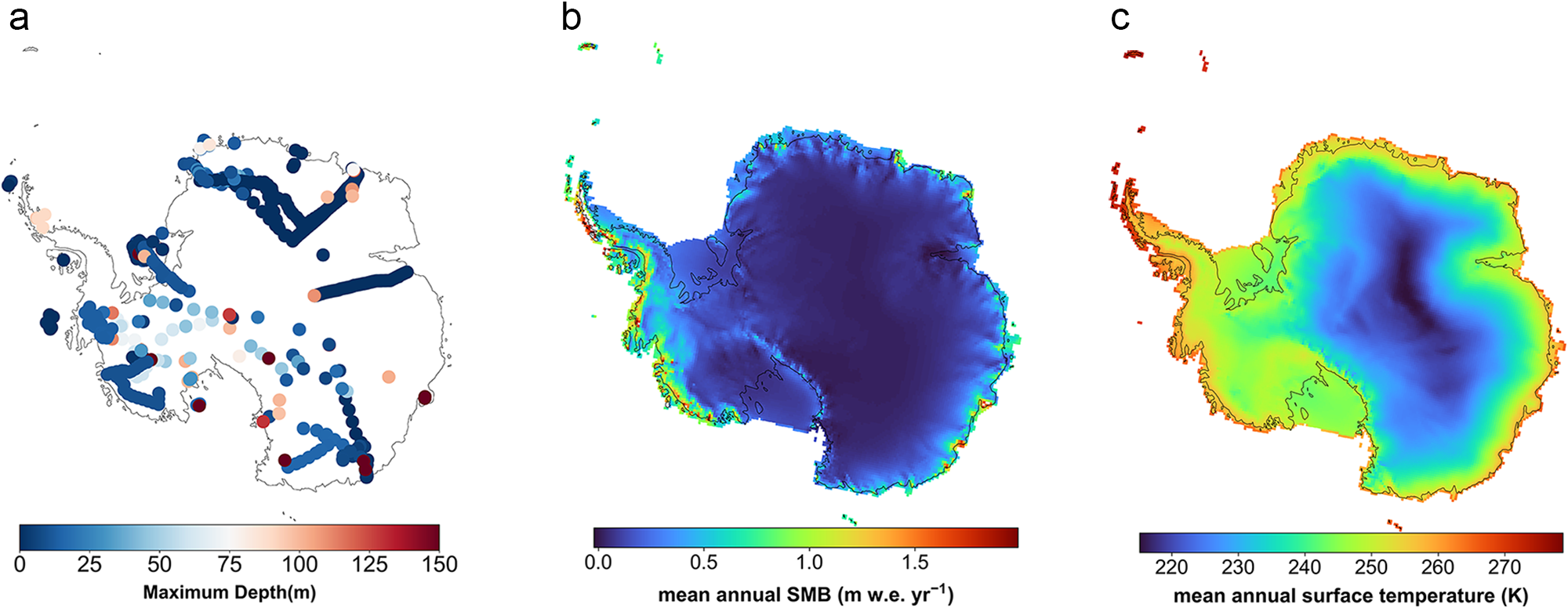
Figure 1. (a) Locations of the 2689 cores used for density predictions extracted from SUMup colored with their maximum depths. (b) Surface mass balance and (c) surface temperature from RACMO2.3.
2.1.1. Density and depth
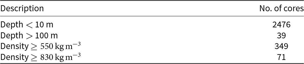
The snow/firn density subdataset was extracted from SUMup. It contains over 2 million unique measurements of density at different depths across both the Antarctic and Greenland ice sheets. These density measurements were obtained using density cutters of different sizes used in snow pits, gravitational methods on ice core sections, neutron-density methods in boreholes, X-ray microfocus computer tomography on snow samples, gamma-ray attenuation in boreholes, pycnometers on snow samples, optical televiewer (OPTV) borehole lagging, and density and conductivity permittivity (DECOMP) (Montgomery and others, Reference Montgomery, Koenig and Alexander2018). The number of cores at important depths and densities are detailed in Table 1.
Table 1. Summary of core depth and density characteristics in SUMup dataset (total of 2689 cores)
2.1.2. Climate variables
• Accumulation rate: The accumulation rate dataset was obtained from the output of the RACMO2.3 model, containing total precipitation (snowfall and rainfall), runoff, melt, refreezing and retention. For our accumulation rate input, we average annual surface mass balance (SMB) outputs from RACMO2.3 for 1979–2016. SMB values were converted to meters of water equivalent per year (m w.e. yr−1). For the purpose of this study, we assume zero ablation in Antarctica and use SMB as the accumulation rate.
• Temperature: For our surface temperature input, we average annual surface temperature outputs from RACMO2.3 for 1979–2016.
Both variables have an initial dimension of (240,262), which we subsequently reshaped into a vector with dimensions (62880,1). The RACMO datasets were combined with the SUMup datasets to create a combined dataset of Antarctic observations containing density, depth, accumulation rate and temperature.
2.2. FirnLearn model development
In this section, we describe the procedures for preprocessing the input data and building, training, validating and testing the machine learning models. In the supplement of this paper, we describe other models employed in predicting density profiles, as well as their relative performance.
2.2.1. Neural network architecture
ANNs are nonlinear statistical models that recognize relationships and patterns between the input and output variables of structured data (Fig. 2) in a manner that models the biological neurons of the human brain (Hatie and others, Reference Hatie, Tibshirani and Friedman2009; O’Shea and Nash, Reference O’Shea and Nash2015). The structure of an ANN consists of (1) an architecture of node layers containing the input layer that receives the data, the output layer that produces an estimate of the dependent variable and hidden layers that take in and sum the weighted inputs and produce an output for other hidden layers or the output layer, (2) an optimization algorithm that determines and updates the weights of the connections between the neurons O’Shea and Nash (Reference O’Shea and Nash2015) and (3) an activation function that determines the output of each neuron.
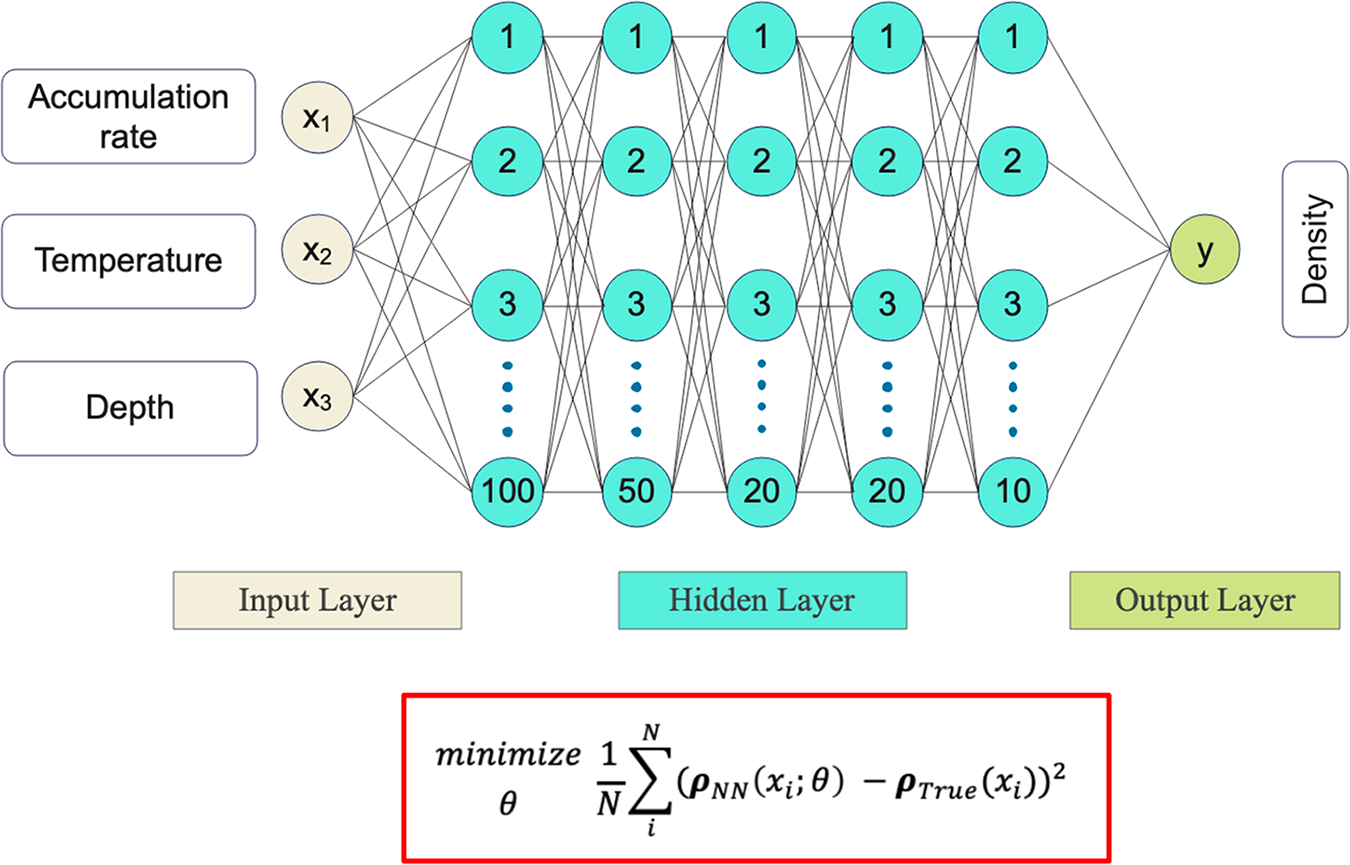
Figure 2. FirnLearn’s artificial neural network architecture. FirnLearn’s goal is to minimize the cost function (in red box). Here,  $\rho_{NN}$ is the density predicted by the neural network, xi is each individual feature, θ is the weight of the neural network and ρTrue is the observed density value.
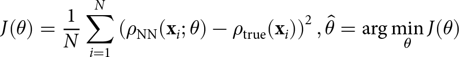
The goal of the training process is to continuously update the weights in every iteration to minimize a loss function, which in most cases, as in our case, is the mean-squared error. This cost function is expressed as
 \begin{equation}
\quad
J(\theta) = \frac{1}{N} \sum_{i=1}^{N} \left(\rho_{\text{NN}}(\mathbf{x}_i; \theta) - \rho_{\text{true}}(\mathbf{x}_i)\right)^2,
\hat{\theta} = \arg\min_\theta J(\theta)
\end{equation}
\begin{equation}
\quad
J(\theta) = \frac{1}{N} \sum_{i=1}^{N} \left(\rho_{\text{NN}}(\mathbf{x}_i; \theta) - \rho_{\text{true}}(\mathbf{x}_i)\right)^2,
\hat{\theta} = \arg\min_\theta J(\theta)
\end{equation} where  $\hat{\theta}$ represents the optimal parameters of the neural network, θ denotes the sets of parameters (weights) of the neural network that the optimization algorithm is adjusting to minimize the cost function, $J(\theta)$ is the cost function, N is the total number of data points in the dataset. xi is the input vector for the ith data point, where i is the index of the current data point that runs from 1 to N, and x is contains the features accumulation rate, temperature and depth. Latitude and longitude are not included as they are already captured in the accumulation rate and temperature. To test this, we included them in a version of our model and found a marginal improvement that was less general. Moreover, when the results from this model were geographically plotted, there were boundary artifacts which may point to scaling issues that cause the NN to overfit to coordinate-specific patterns.
The variables that determine the structure and performance of a model are called hyperparameters and they include the number of neurons per layer, number of layers, activation function, optimizer, learning rate, batch size and number of epochs.
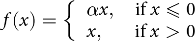
FirnLearn, shown in Figure 2, is a seven-layered ANN coded in python using using tensorflow keras and sci-kit learn. The hyperparameters used to construct FirnLearn were tuned using cross validation to find the best performing combination of hyperparameters, i.e. the hyperparameter combination with the lowest root-mean-square error (RMSE—see Section 2.3). It consists of one input layer with three neurons corresponding to the number of selected features, accumulation rate, temperature and depth; five hidden layers with 100, 50, 20, 20, 10 neurons, respectively; and one output layer corresponding to density. Leaky ReLU was chosen as the activation function for the hidden layers. ReLU, short for rectified linear unit, is a piecewise function that outputs the input value if it is greater than 0. It is given by:
 \begin{equation}
f(x) =
\left\{
\begin{array}{lr}
\alpha x, & \text{if } x \leqslant 0\\
x, & \text{if } x \gt 0
\end{array}
\right.
\end{equation}
\begin{equation}
f(x) =
\left\{
\begin{array}{lr}
\alpha x, & \text{if } x \leqslant 0\\
x, & \text{if } x \gt 0
\end{array}
\right.
\end{equation}where α is a small constant (e.g. 0.01) ensuring the gradient is nonzero for negative values.
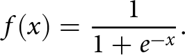
For the output layer, the sigmoid function was chosen as the activation function. It is represented as
 \begin{equation}
f(x) = \frac{1}{1+e^{-x}}.
\end{equation}
\begin{equation}
f(x) = \frac{1}{1+e^{-x}}.
\end{equation}We used the Adam optimizer technique (Kingma and Ba, Reference Kingma and Ba2017) to optimize the weights for gradient descent. We also tuned the learning rate, which determines how much the weights are changed in each iteration. The best performing learning rate was 0.0001 among a starting range of 0.01, 0.001 and 0.0001.
FirnLearn predicts firn density (ρ) using the function  $\rho = f(A,T,z)$ where A represents the accumulation rate, T represents temperature, and z represents depth. For surface density predictions (z = 0), the model simplifies to $\rho = f(A,T,0)$. These inputs capture the primary drivers of firn densification processes, aligning with the benchmark Herron and Langway Reference Herron and Langway(1980) model.
2.2.2. Training and testing
After the dataset was extracted, we split it into training, testing and validation sets. The training set is used to train the model, allowing it to learn patterns and relationships in the data. The validation set is used during training to tune model hyperparameters and prevent overfitting by providing an independent evaluation of the model’s performance. Finally, the testing set is used after training to assess the model’s performance on unseen data and evaluate its generalization capabilities. Before training commenced, sklearn’s StandardScaler was used to normalize the input variables and MinMaxScaler was used to normalize the output variable from 0 to 1. We conducted a 72-8-20 split on the cores for the training-testing-validation sets. The validation cores (536 cores) were selected at random, while the testing cores (225 cores) were selected to ensure 9 of the cores were at least 50 m deep, and 1 was below 50 m in order to provide visual representation of FirnLearn’s performance with depth, as shown in Figure 3. We selected these sites to be representative of the full spread of regions in Antarctica, selecting one site from the Antarctic Peninsula, East Antarctica, West Antarctica, the South Pole and near the Ross Sea. This also let us test a range of surface density values from around  $320\,\mathrm{kg\,m}^{-3}$ to greater than $550\,\mathrm{kg\,m}^{-3}$. Our tests were conducted on one from the Larsen C Ice Shelf (66.58∘ S, 63.21∘ W), Marie Byrd Land (78.12∘ S, 120∘ W), Ellsworth land (78.1∘ S, 95.65∘ W), Taylor Dome (77.88∘ S, 158.46∘ E), near Vostok Station (82.08∘ S, 101.97∘ E), Dumbont D’Urville Station (66.66∘ S, 140∘ E), two cores in the Queen Maud Land region [(73.1∘ S, 39.8∘ E); 75∘ S, 0∘] and two cores from the South Pole [(88.51∘ S, 178.53∘ E), (90∘ S, 0)]. Across all 225 test cores, the RMSE was $30\,\mathrm{kg}\,\mathrm{m}^{-3}$ and the explained variance was 98%.
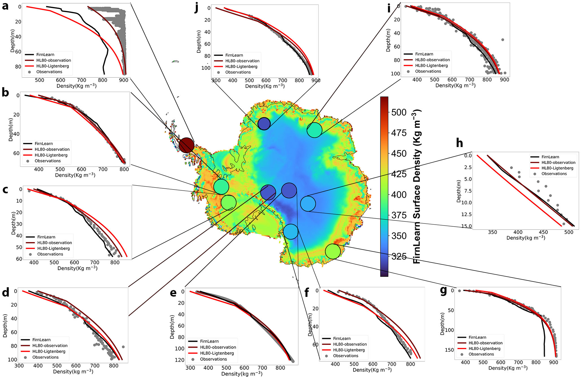
Figure 3. Depth–density profiles at the six test sites. Shown corresponding to each site are the observed density profile in gray, the FirnLearn modeled density in red and the HL modeled density in black for (a) a core on the Larsen C Ice Shelf (66.58∘ S, 63.21∘ W), (b) a core on the Ellsworth Land (78.1∘ S, 95.65 W), (c) a core on the Marie Byrd Land (78.12∘ S, 120∘ W), (d) a core near the South Pole (88.51 S, 178.53 E), (e) the South Pole (90∘ S, 0), (f) the Taylor Dome (77.88∘ S, 158.46∘ E), (g) Dumbont D’Urville Station (66.66∘ S, 140∘ E), (h) a core near VostokStation (82.08 S, 101.97 E), (i) a core on the Queen Maud Land (73.1∘ S, 39.8∘ E) and (j) a core on the Queen Maud Land (75∘ S, 0).
2.3. Evaluation
We evaluate our model’s performance using several metrics. We use the coefficient of determination r 2 to quantify how well the model predicts the dependent variable (density). It is given by
 \begin{equation}
r^2 = 1 - \frac{\sum_{i=1}^{N} (\rho_i - \hat{\rho}_i)^2}{\sum_{i=1}^{N} (\rho_i - \bar{\rho})^2}
\end{equation}
\begin{equation}
r^2 = 1 - \frac{\sum_{i=1}^{N} (\rho_i - \hat{\rho}_i)^2}{\sum_{i=1}^{N} (\rho_i - \bar{\rho})^2}
\end{equation} where ρi is the actual density value at each data point,  $\hat{\rho}_i$ is the predicted density value for each data point and $\bar{\rho}$ is the mean of the actual density values.
The RMSE is an average measure of the difference between the observed density and the predicted density, given by
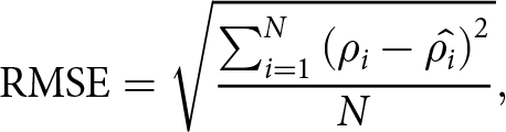 \begin{equation}
\mbox{RMSE} = \sqrt{\frac{\sum_{i=1}^N \left(\rho_i - \hat{\rho_i}\right)^2}{N}},
\end{equation}
\begin{equation}
\mbox{RMSE} = \sqrt{\frac{\sum_{i=1}^N \left(\rho_i - \hat{\rho_i}\right)^2}{N}},
\end{equation} where N is the number of model-observation pairs, ρi is the true density value,  $\hat{\rho_i}$ is the predicted density value and $\bar{\rho_i}$ is the mean of the observed density values. We evaluate the RMSE for an independent test set with a split discussed in Section 2.2.2. To estimate the difference between modeled and observed surface density and FAC, we use the relative bias metric. The relative bias is given as
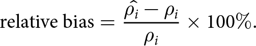 \begin{equation}
\mbox{relative bias} = \frac{\hat{\rho_i} - \rho_i}{\rho_i}\times 100\%.
\end{equation}
\begin{equation}
\mbox{relative bias} = \frac{\hat{\rho_i} - \rho_i}{\rho_i}\times 100\%.
\end{equation}A positive relative bias indicates an overestimation by the model, while negative bias indicates an underestimation by the model. The bulk relative bias is the total average reative bias for all cores
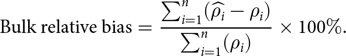 \begin{equation}\text{Bulk relative bias}=\frac{\sum_{i=1}^n(\widehat{\rho_i}-\rho_i)}{\sum_{i=1}^n(\rho_i)}\times100\%.\end{equation}
2.4. Herron and Langway, 1980
Herron and Langway Reference Herron and Langway(1980), denoted HL in this study, is a benchmark empirical firn densification model, upon which many contemporary models are built due to its foundational assumptions. The assumptions made in HL are as follows: (1) the densification rate is a function of the porosity, and (2) the densification rate has an Arrhenius dependence on the temperature. These assumptions are combined to form the equation
 \begin{equation}
\frac{{d}\rho}{{d}t} = C(\rho_\mathrm{ice} - \rho),
\end{equation}
\begin{equation}
\frac{{d}\rho}{{d}t} = C(\rho_\mathrm{ice} - \rho),
\end{equation} where  $\rho_\mathrm{ice}$ is the density of ice ( $917\,\mathrm{kg\,m}^{-3}$), ρ is the density at a given depth and C is a site-specific constant. It is worth noting that while $\frac{{d}\rho}{{d}t}$ may seem time dependent, the time-dependent change in density is captured in the depth variability of density
 \begin{equation}
C = k \exp\left(-\frac{Q}{RT}\right)A^a,
\end{equation}
\begin{equation}
C = k \exp\left(-\frac{Q}{RT}\right)A^a,
\end{equation} where k in Eqn (9) is a temperature-dependent Arrhenius-type rate constant, a is a constant dependent on the densification mechanism, Q is the Arrhenius activation energy (kJ mol−1), R is the gas constant (8.314 kJ mol−1 K−1), T is the mean annual temperature at the site (K) and A is the accumulation rate in waters equivalent. The site-specific constant, C, for  $\rho \leqslant$ $550\,\mathrm{kg\,m}^{-3}$, is given by
 \begin{equation}
C = 11\exp\left(-\frac{10.16}{RT}A\right),
\end{equation}
\begin{equation}
C = 11\exp\left(-\frac{10.16}{RT}A\right),
\end{equation} and for  $\rho \gt 550\,\mathrm{kg\,m}^{-3}$, we have
 \begin{equation}
C = 575\exp\left(-\frac{21.4}{RT}A^{0.5}\right).
\end{equation}
\begin{equation}
C = 575\exp\left(-\frac{21.4}{RT}A^{0.5}\right).
\end{equation} HL requires a surface density boundary condition. In order to obtain predictions for depth–density profiles, we used both surface density values from observations, as well as surface density predictions from Ligtenberg and others Reference Ligtenberg, Helsen and van den Broeke(2011). However, for predicting depths at  $550\,\mathrm{kg\,m}^{-3}$ and $830\,\mathrm{kg\,m}^{-3}$, we used surface density predictions from FirnLearn, which allowed for a direct comparison.
3. Results and discussion
3.1. Depth–density profiles
We use FirnLearn and HL to simulate firn profiles at ten test sites and compare the results in Figure 3 and Tables 2, 3 and 4. This allows us to visually evaluate the difference in performance between HL and FirnLearn. For HL, we evaluated the HL function using two different surface density values, and the two curves are named HL80-observation and HL80-Ligtenberg. For the HL80-observation curves, we use the surface density value directly from the observations, while for the HL80-Ligtenberg curves, we set the surface density values to surface density predictions from Ligtenberg and others Reference Ligtenberg, Helsen and van den Broeke(2011). The FirnLearn curves, depicted as black lines, are generated by applying function evaluations of the FirnLearn model, taking in specified accumulation rates, temperatures and depths, i.e.  $\rho = f(A,T,z)$. All three models do a good job of predicting the observations. FirnLearn outperforms both HL80 models across the full depth range, in locations c, d, e and j (Fig. 3 and Table 2). HL80-observation outperforms FirnLearn and HL80-Ligtenberg at locations a, b, f and g, while FirnLearn performs comparably to HL80-observation at locations h and i.
Table 2. RMSE values for the density profile predictions in Figure 3
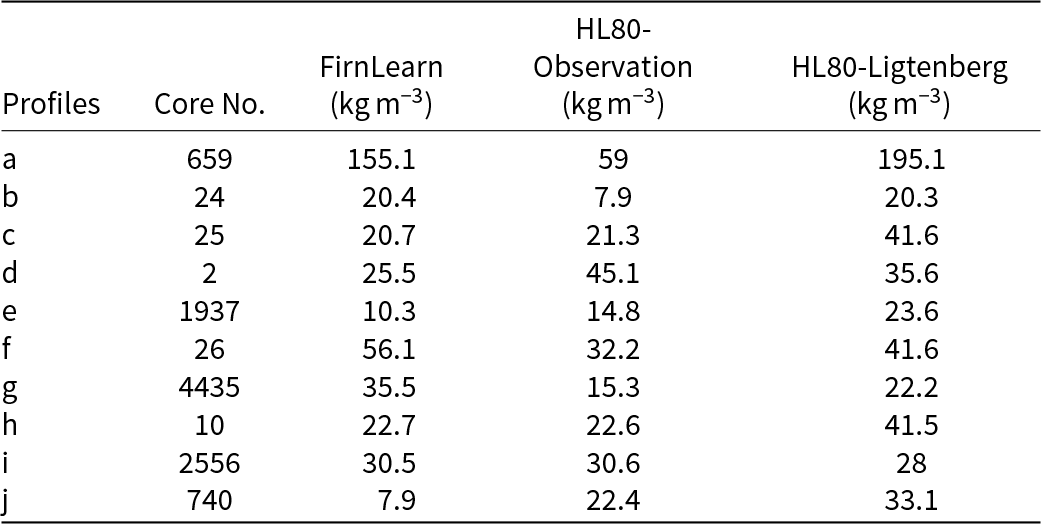
Table 3. RMSE values for the first stage of densification ( $\leqslant 550\,\mathrm{kg}\,\mathrm{m}^{-3}$) density profile predictions in Figure 3
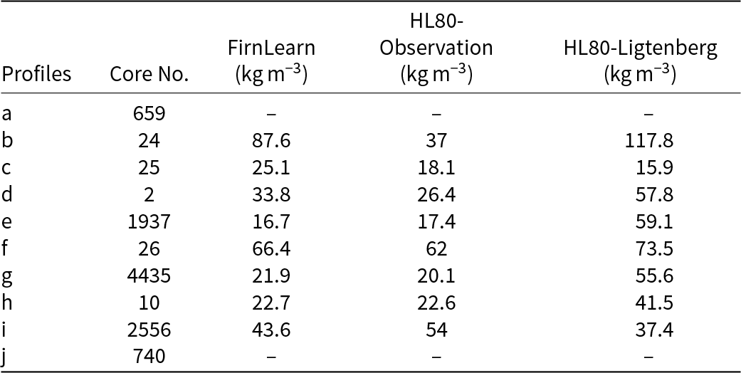
Table 4. RMSE values for the second stage of densification ( $ \gt 550\,\mathrm{kg}\,\mathrm{m}^{-3}$) density profile predictions in Figure 3
Of the three model predictions plotted for each core, although FirnLearn performs well, HL80-observation leads in the first stage of densification due to accurate surface density inputs in cores b, c, d, f and g (Table 3), with FirnLearn having a comparable performance at these locations. FirnLearn outperforms in the second stage across most locations (Table 4c, d, e and j) and is comparable or better than HL80-observation in overall performance, while HL80-Ligtenberg generally underperforms consistently due to a greater mismatch in surface density predictions.
A more pronounced discrepancy in performance is evident in Figure 3a for the Larsen C Ice Shelf. This location was included to represent conditions on an ice shelf with meltwater conditions, as well as conditions that may become more frequent with climate change. Here, owing to the accurate surface density input, HL80-observation predicts the density trend with greater accuracy than HL80-Ligtenberg and FirnLearn. On the other hand, at location g, the Dumbont D’Urville Station, FirnLearn underperforms in the third stage of densification ( $ \gt 830\,\mathrm{kg}\,\mathrm{m}^{-3}$). This underperformance is attributed to the limited number of observations under conditions similar to those at this site in Antarctica. As discussed in Section 1 and evidenced in the SUMup density dataset, surface density measurements have only been collected for a small percentage of the AIS. Figure 3 shows that without accurate surface density observations, FirnLearn is a better density prediction model than Herron and Langway Reference Herron and Langway(1980).
It is worth highlighting that FirnLearn offers the added advantage of providing density information at specific depths for a given site without requiring surface density or density data from previous depths. This characteristic further enhances the speed and utility of FirnLearn in densification research. Additionally, it could be useful in ice core drilling operations for optimized site selection and resource allocation.
3.2. Surface density
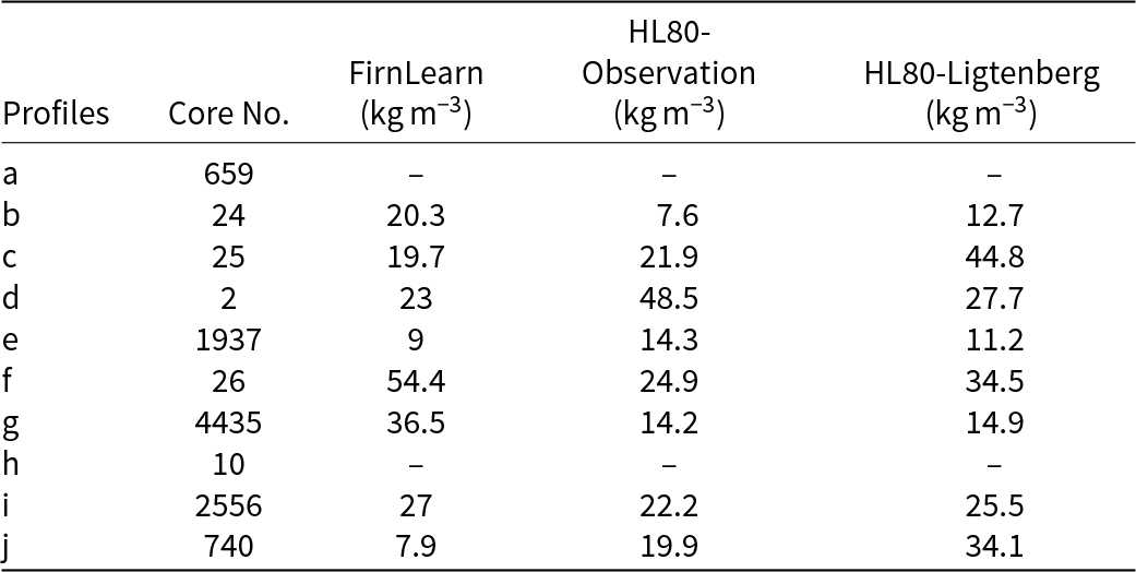
We predict surface density across the AIS by putting accumulation rate and temperature from RACMO2.3 (Noël and others, Reference Noël2018) at z = 0 into the trained and validated FirnLearn model. These predictions are based on the equation  $\rho = f(A,T,0)$, where the function f is FirnLearn, A represents the accumulation rate and T represents the temperature. Across Antarctica, the surface density exhibits a notable spatial variation (Fig. 4a). In the interior of East Antarctic, we observe relatively lower values in the range 320– $380\,\mathrm{kg\,m}^{-3}$, reflecting the region’s colder surface temperatures. In contrast, we find higher surface density values, exceeding $450\,\mathrm{kg\,m}^{-3}$, along the coastal areas and on ice shelves. We attribute these higher densities to the higher temperatures, higher accumulation rates and the higher wind speeds prevalent in these regions (McDowell and others, Reference McDowell, Albert, Lieblappen and Keegan2020). For the majority of the sites, the relative bias is within $\pm25\%$, with only one site having a relative bias above $100\%$ (Fig. 4b). For this site in the Southeastern Antarctica, FirnLearn overpredicts the surface density by 174%.
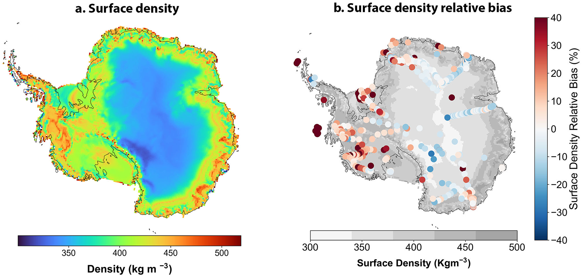
Figure 4. (a) The FirnLearn predicted surface density field for Antarctica and (b) relative bias between the predicted surface density and the observed surface density.
Semi-empirical models require a prescribed surface density boundary condition, making these surface density predictions a key output of FirnLearn. The importance of the surface density boundary condition was underscored by Thompson-Munson and others Reference Thompson-Munson, Wever, Stevens, Lenaerts and Medley(2023). They employed two models, the physics-based SNOWPACK (Bartelt and Lehning, Reference Bartelt and Lehning2002) with a surface density that varies based on atmospheric conditions and the Community Firn Model configured with a semi-empirical densification equation (CFM-GSFC; Stevens and others Reference Stevens, Verjans, Lundin, Kahle, Horlings, Horlings and Waddington(2020)) run with a constant surface density of  $350\,\mathrm{kg\,m}^{-3}$. Their analysis of firn properties across the GrIS revealed that SNOWPACK simulated more variability between firn layers compared to CFM-GSFC, although some of this variability could be associated with SNOWPACK’s microstructure dependence. Importantly, our predictions are similar to prior research findings (Kaspers and others, Reference Kaspers, van de Wal, van den Broeke, Schwander, van Lipzig and Brenninkmeijer2004; van den Broeke, Reference van den Broeke2008; Ligtenberg and others, Reference Ligtenberg, Helsen and van den Broeke2011) that have employed parameterizations based on combinations of surface temperature, accumulation rate, wind speed to derive surface density predictions.
3.3. Depths at 550 kg m−3 and 830 kg m−3
Figure 5a depicts the depth at  $550\,\mathrm{kg\,m}^{-3}$ with a depth range from 0 to 30 m, with higher values (18–30 m) concentrated in East Antarctica and lower values (0–15 m) prevalent in West Antarctica and along the coast. This spatial distribution is similar to the pattern of surface density, reflecting an expected relationship between the two variables. Figure 5c shows the depth at $830\,\mathrm{kg\,m}^{-3}$ which ranges from 20 to 122 m, with higher values (80–122 m) predominantly found in East Antarctica. The spatial distribution of z 830 is different than z 550 in that for z 830, there are higher values in regions of West Antarctica, the Antarctic Peninsula and certain coastal areas. This is primarily attributed to the higher accumulation rates, which result in the rapid burial of fresh snow. Consequently, densification rates reduce with depth. These trends align with the trends observed in earlier models such as van den Broeke Reference van den Broeke(2008) and Ligtenberg and others Reference Ligtenberg, Helsen and van den Broeke(2011). In the vicinity of the major ice shelves, such as the Ross, Filchner–Ronne, Larsen and Amery Ice Shelves , z 550 ranges from 5 to 13 m in FirnLearn, a close range to both van den Broeke Reference van den Broeke(2008) and Ligtenberg and others Reference Ligtenberg, Helsen and van den Broeke(2011), while z 830 ranges from 60 to 90 m in FirnLearn, 50 to 70 m in van den Broeke Reference van den Broeke(2008) and Ligtenberg and others Reference Ligtenberg, Helsen and van den Broeke(2011). The discrepancy in z 830 values may stem from limited data availability at these depths. Figure 5b compares the observed and modeled z 550 for 220 locations with densities beyond $550\,\mathrm{kg\,m}^{-3}$, while Figure 5d compares the observed and modeled z 830 for 88 locations with densities beyond $830\,\mathrm{kg\,m}^{-3}$. For z 550, there is a clustering of points along the line of perfect agreement, particularly in the mid-range observed depth values (5–15 m), indicating strong predictive accuracy in this range. FirnLearn exhibits slightly tighter clustering compared to HL80, as reflected in its lower RMSE value (4.1 m vs 4.3 m for HL80). However, at depths below 5 m, there are more points lying above the upper confidence interval for both FirnLearn and HL, indicating that both models typically overestimate the depth values along the coast where the conditions are warmer and wetter, and accumulation rates are higher. This is possibly due to an underestimation of surface density, causing the models to densify slower than in observations. At greater depths, FirnLearn performs better than HL with more HL values lying below the line of perfect agreement. For z 830, there is a similar trend with more points above the upper confidence interval for lower to mid-range observed depth values (0–60 m) and a cluster around the line of perfect agreement for the remaining points. FirnLearn typically overpredicts z 830 as compared to HL, which as mentioned earlier may be a result of the sparsity of data at deeper depths.
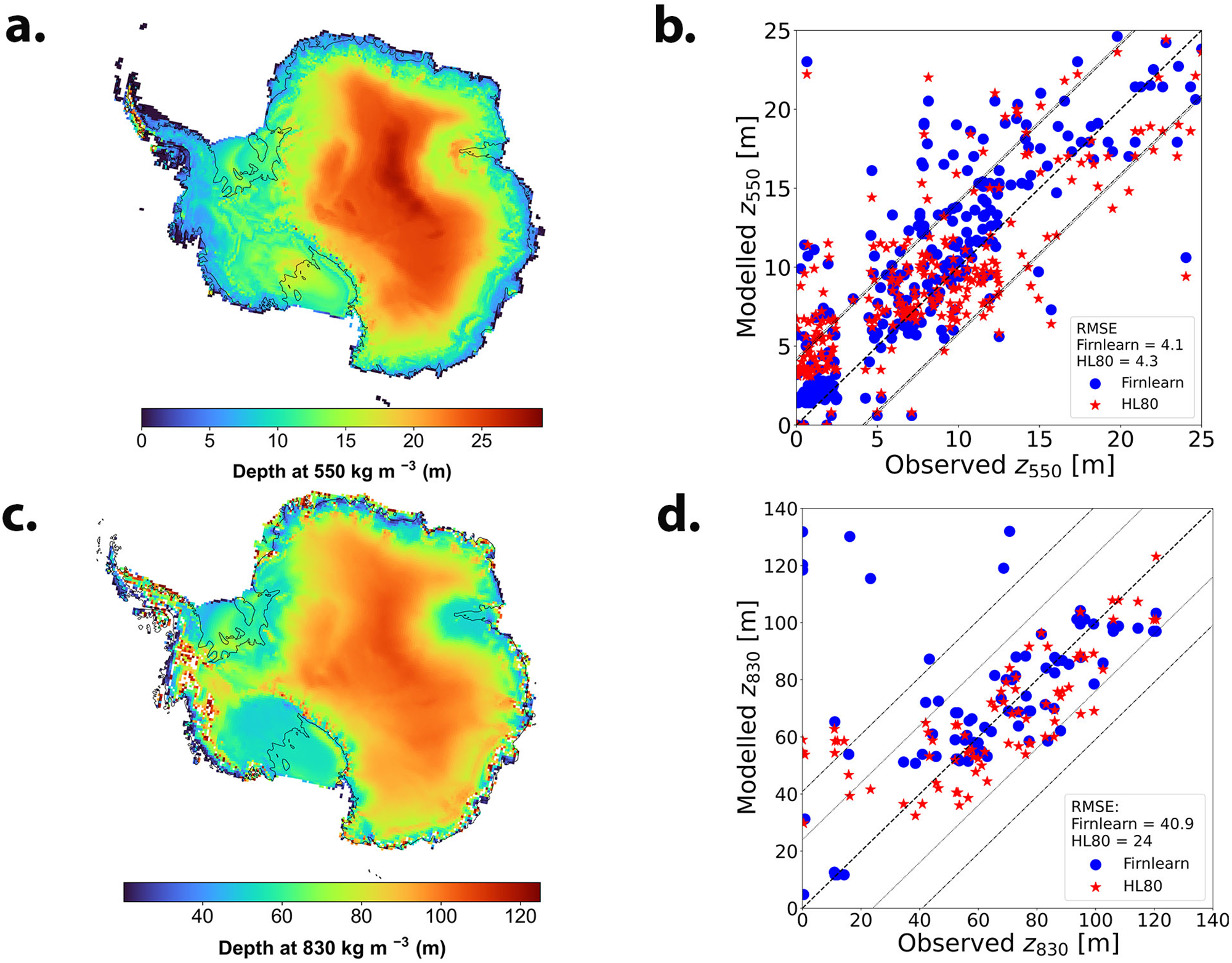
Figure 5. (a) The predicted depth at  $550\,\mathrm{kg\,m}^{-3}$ in meters. (b) Comparison of modeled to observed depth at $550\,\mathrm{kg\,m}^{-3}$. (c) The predicted depth at $830\,\mathrm{kg\,m}^{-3}$ in meters. (d) Comparison of modeled to observed depth at $830\,\mathrm{kg\,m}^{-3}$. Here the FirnLearn computed surface density is used for the Herron and Langway Reference Herron and Langway(1980) model.
3.4. Firn air content
We explore predictions of FAC, the amount of air-filled pore space within the firn layer, using FirnLearn and HL, and compared them to the FAC from observations. FAC is an important parameter as it is essential for deriving the mass-balance estimates of an ice sheet (Helsen and others, Reference Helsen2008; Horlings and others, Reference Horlings, Christianson, Holschuh, Stevens and Waddington2020) which improves our understanding and estimates of gas exchange dynamics and climate records (Trudinger and others, Reference Trudinger, Etheridge, Rayner, Enting, Sturrock and Langenfelds2002; Buizert and others, Reference Buizert, Sowers and Blunier2013). It is also essential for estimating meltwater content of ice sheets, hence ice sheet contribution to sea-level rise (Medley and others, Reference Medley, Neumann, Zwally, Smith and Stevens2022). To facilitate comparison between FirnLearn and HL, we employed the surface density predictions generated by FirnLearn as the surface density conditions for HL. The FAC is calculated by integrating porosity over the depth of the firn column and is represented as:
 \begin{equation}
\mbox{FAC} = \int_{z_l}^{z_u}\frac{\rho_\mathrm{ice}-\rho(z)}{\rho_\mathrm{ice}}\mathrm{d}z
\end{equation}
\begin{equation}
\mbox{FAC} = \int_{z_l}^{z_u}\frac{\rho_\mathrm{ice}-\rho(z)}{\rho_\mathrm{ice}}\mathrm{d}z
\end{equation} where  $\rho_\mathrm{ice}$ is the density of ice ( $917\,\mathrm{kg\,m}^{-3}$) and $\rho(z)$ is the firn density at a given depth, and the depth interval is set by an upper bound depth zu and a lower bound depth $z_l = 0$, representing the surface.
As depicted in Figure 6a and Table 1, the majority of density cores used in this study are relatively shallow - approximately 90% less than 10m deep. This shallow depth distribution explains the generally low observed FAC values in Figure 6b. Hence, for a direct comparison between the modeled (FirnLearn and HL), and observed FAC, we evaluated the FAC of each core up to its respective maximum depth from SUMup, using FirnLearn’s surface density as the boundary condition for HL’s FAC calculations. This results in the difference in FirnLearn’s and HL’s evaluation of FAC being a reflection of their accuracy in predicting the densities in the first stage of densification. Very little difference is visually evident between the observed FAC and FirnLearn’s and HL’s predicted FAC (Figs. 6b, c and d).
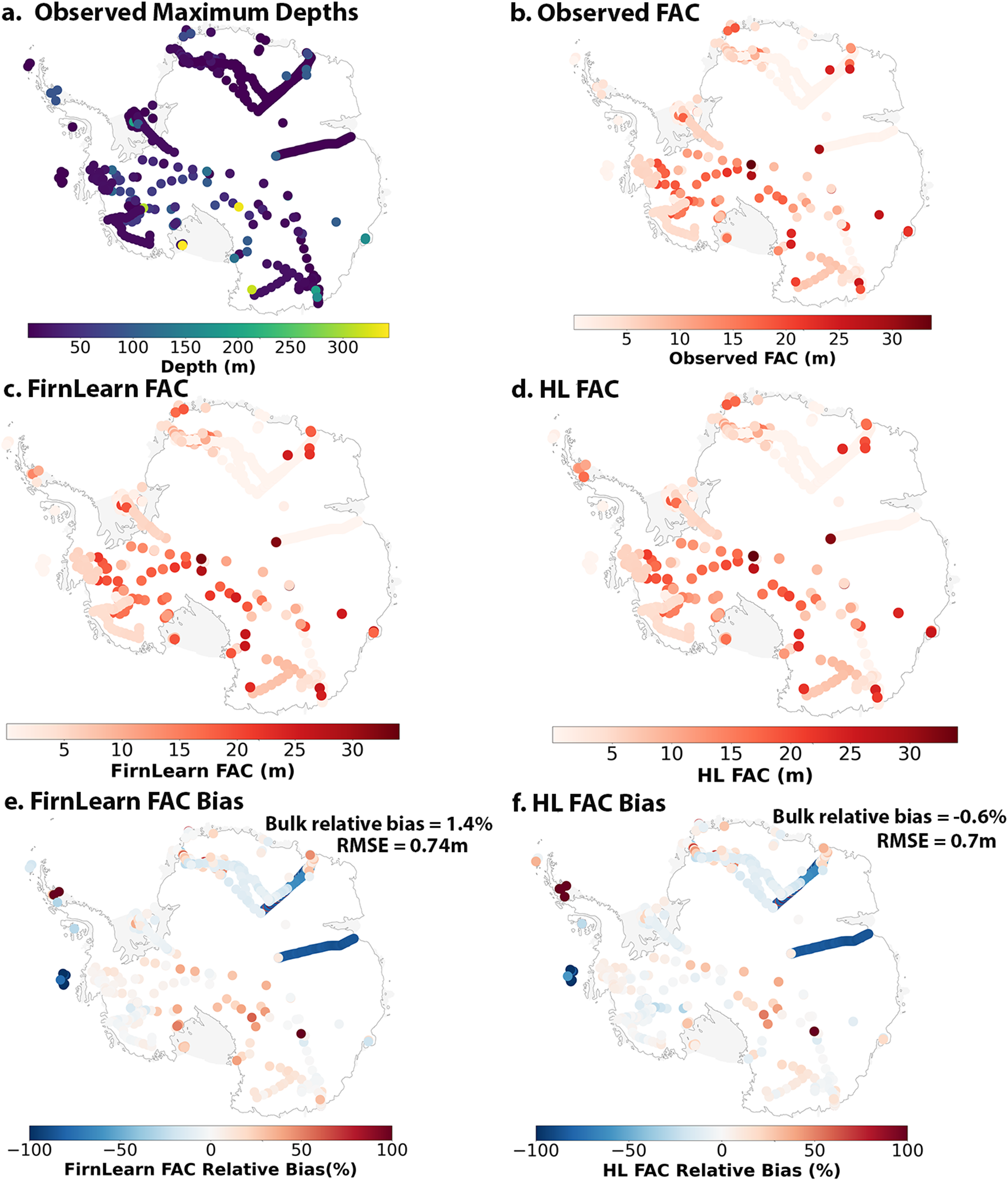
Figure 6. Firn air content across Antarctica, comparing models to observations and assessing bias: (a) Spatial distribution of 2689 SUMup cores, with shading denoting core depth, (b) observed FAC from calculated from the densities of the SUMup cores, (c) FAC in meters, calculated with FirnLearn, (d) FAC in meters, calculated with Herron and Langway Reference Herron and Langway(1980), (e) relative bias between the FAC calculated with FirnLearn and the observed FAC and (f) relative bias between the FAC calculated using Herron and Langway Reference Herron and Langway(1980) and the observed FAC.
Figures 6e and f depict the spatial distribution of relative bias values for FirnLearn’s FAC and HL’s FAC, respectively. Given that we used FirnLearn’s surface density as the boundary condition for HL’s FAC calculations, FirnLearn’s FAC bias values are similar to HL’s FAC bias values, with HL slightly underestimating FAC with a bulk relative bias of -0.6% and FirnLearn slightly overstimating FAC with a bulk relative bias of 1.4%. This disparity is driven by relatively deeper cores (z>50), where FirnLearn slightly overestimates FAC, while HL slightly underestimates FAC. The RMSE values are also similar, at 0.74m for FirnLearn and 0.7m for HL, suggesting both models perform comparably well across the full dataset. To obtain a broader representation of the full firn column, we calculated FAC over a wider accumulation rate (0–3 m w.e. yr −1) and temperature (215–273 K [−58 to  $0^{\circ}\mathrm{C}$]) parameter space from the surface to 100 m depth. It is worth noting that some of these conditions are extreme in Antarctica. The heat maps shown in Figure 7 depict the FAC from FirnLearn, Herron and Langway Reference Herron and Langway(1980), and the difference between the two. As shown in these figures, FirnLearn and HL produce similar FAC patterns, with FAC being highest at low temperatures and lowest at low accumulation rates and high temperatures. Relating this to ice sheets, FAC is predicted by both models to be ∼30–50 m on the interior, where accumulation rates and temperatures are low (<0.5 m w.e. yr−1 and <225 K [ $-48^{\circ}\mathrm{C}$], respectively), and in coastal regions where accumulation rates could be as high as 2 m w.e. yr−1, and temperatures could be higher than 270 K [ $-23^{\circ}\mathrm{C}$]. In West Antarctica, with accumulation rates between 0.5 and 2 m w.e. yr−1 and temperatures higher than 250 K [ $-23^{\circ}\mathrm{C}$], FAC is predicted by FirnLearn and HL to be greater than 40 m.
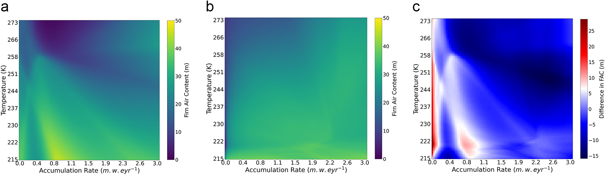
Figure 7. (a) FAC in meters, calculated with FirnLearn, (b) firn air content in meters, calculated with Herron and Langway Reference Herron and Langway(1980) and (c) difference in FAC in meters, between the FAC calculated using FirnLearn and the FAC calculated using Herron and Langway Reference Herron and Langway(1980). The difference is presented as FirnLearn minus HL80. (a) FirnLearn FAC (m), (b) HL FAC (m) and (c) difference in FAC.
Figure 7c shows that on average, FirnLearn’s FAC is in agreement with HL’s FAC, with minor disagreements where FirnLearn underpredicts when compared to HL. The regions with the highest positive differences (FirnLearn  $\gg$ Herron and Langway Reference Herron and Langway(1980)) are at lower accumulation rates, as indicated by the red hues. Conversely, the regions with the highest negative differences (FirnLearn $\ll$ Herron and Langway Reference Herron and Langway(1980)) are at mid to higher accumulation rates, as indicated by the blue hues, a region which coincides with the parameter space of the training data. It is worth noting that conditions where accumulation rates are very low (< 1 m w.e. yr −1) and temperatures are very high (> 260 K [ $-13^{\circ}\mathrm{C}$]) or where accumulation rates are very high (> 1 m w.e. yr −1) and temperatures are very low (< 230 K [ $-43^{\circ}\mathrm{C}$]) rarely exist in Antarctica, at least not within its current climate regime. Figure 7 is shown in order to understand FAC values within a wider accumulation rate and temperature parameter space.
4. Limitations to FirnLearn
Despite its promising performance, FirnLearn has limitations due to data quality and quantity. As shown in Figure 1, the spatial distribution of density observations is notably limited, particularly in East Antarctica. Additionally, as shown in Figure 6a, the majority of density observations in the dataset are concentrated at shallow depths. Consequently, the discrepancies between FirnLearn’s density predictions and observations increase as depth increases, as evident by the higher RMSE in the predictions of depth at  $830\,\mathrm{kg\,m}^{-3}$ compared to the predictions of depth at $550\,\mathrm{kg\,m}^{-3}$ (Fig. 5). Also, as seen in Tables 2, 3 and 4, FirnLearn still underperforms HL80 in certain conditions. For these conditions, for instance, regions with sparse-depth observations ( $ \gt 830\,\mathrm{kg}\,\mathrm{m}^{-3}$), using a weighted combination of HL80 and FirnLearn predictions could provide better results. This approach would leverage the strengths of both methods, compensating for FirnLearn’s inaccuracies at greater depths with HL80’s depth performance, while benefiting from FirnLearn’s surface density predictions and better performance in stage 2 ( $550 \leqslant \rho \lt 830\,\mathrm{kg}\,\mathrm{m}^{-3}$). With the growth of the SUMup dataset as more firn data are collected, FirnLearn’s density predictions are bound to improve, as it is trained on new data.
FirnLearn is also limited to a steady-state assumption, therefore unable to predict temporal firn density evolution. Density observations from SUMup are collected over several years, and at different periods of the year, leading to knowledge gaps regarding seasonal variability in firn properties. Without explicit time-dependent inputs, FirnLearn struggles to generalize to evolving firn conditions. However, with additional training on newer datasets that include temporal markers, its ability to capture temporal firn density evolution is expected to improve.
It is also worth noting that while FirnLearn’s surface density predictions are in line with surface density predictions from (Kaspers and others, Reference Kaspers, van de Wal, van den Broeke, Schwander, van Lipzig and Brenninkmeijer2004; van den Broeke, Reference van den Broeke2008; Ligtenberg and others, Reference Ligtenberg, Helsen and van den Broeke2011), its predictions may still be less reliable in parts of East Antarctica due to the limited number of data points in that region.
Another challenge lies in the lack of interpretability of deep learning models like FirnLearn. These models are effectively ‘black boxes’, such that it is difficult to understand the underlying processes governing model predictions. However, given the black-box nature, ANNs serve as effective tools in contexts where predictive accuracy outweighs model interpretability, which is likely the case for depth–density profiles in Antarctica at this time. The improved accuracy offered by ANNs holds the potential to produce improved parameters for understanding firn densification physics.
5. Conclusions
In this study, we introduced FirnLearn, a new steady-state densification model for the Antarctic firn layer based on deep learning of data from observations and output from the RACMO. Comparison with observations highlights FirnLearn’s improved predictability of firn density at intermediate depths, where discrepancies between observations and traditional models, such as Herron and Langway Reference Herron and Langway(1980) are more pronounced. In addition, we have used FirnLearn to accurately derive surface density, depth at  $550\,\mathrm{kg\,m}^{-3}$ and $830\,\mathrm{kg\,m}^{-3}$ (pore close-off) and FAC across Antarctica. This study demonstrates the potential of deep learning techniques in improving Antarctic firn density estimates and strengthens the promising foundation for the development of a generally applicable firn model. In the future, we plan to expand this model by applying it to the Greenland ice sheet and coupling it to physics to develop a physics-informed neural network which can be applied to both dry and wet firn densification.
Supplementary material
The supplementary material for this article can be found at https://doi.org/10.1017/jog.2025.26.
Data availability statement
FirnLearn’s code is available at https://github.com/ayobamiogunmolasuyi/FirnLearn. The repository contains all the scripts used to train the models and produce the plots and results. The SUMup dataset is available at https://github.com/MeganTM/SUMMEDup while the RACMO dataset is here https://doi.pangaea.de/10.1594/PANGAEA.896940.
Acknowledgements
This work was supported by the National Science Foundation (AO, GRFP-2021295396; CRM, 2024132; IB, 1851094), the Army Research Office (CRM, 78811EG), the National Aeronautics and Space Administration (CRM, EPSCoR-80NSSC21M0329). We thank Brice Noel for his assistance in accessing the RACMO data.
Competing interests
The authors declare that they have no conflict of interest.


 Open access