


Introduction
Ground-penetrating radar (GPR) is a primary choice for investigating glacier since the early decades of the last century (Stern, Reference Stern1929). The electromagnetic (EM) wave has excellent penetration in low-loss media such as ice (Bradford and others, Reference Bradford, Nichols, Mikesell and Harper2009; Saintenoy and others, Reference Saintenoy2013) and its logistic is simpler than those associated with other techniques. Common-offset and common-mid-point (CMP) GPR profiling surveys have been conducted in several flavors at hundreds of glacial and periglacial sites around the world (Watts and England, Reference Watts and England1976; Murray and others, Reference Murray, Gooch and Stuart1997; Forte and others, Reference Forte, Pipan, Francese and Godio2015). These surveys have focused on bedrock reconstruction (Ramírez and others, Reference Ramírez2001; Fischer, Reference Fischer2009), internal layering mapping (Arcone, Reference Arcone1996; Hambrey and others, Reference Hambrey2005), glacial inclusions (Murray and others, Reference Murray, Gooch and Stuart1997), water distribution (Moran and others, Reference Moran, Greenfield and Arcone2000; Irvine-Fynn and others, Reference Irvine-Fynn, Moorman, Williams and Walter2006) and englacial channel detection (Stuart and others, Reference Stuart, Murray, Gamble, Hayes and Hodson2003). Time-lapse GPR measurements have also been undertaken to monitor the water levels in glacial cavities (Garambois and others, Reference Garambois, Legchenko, Vincent and Thibert2016) to prevent catastrophic flooding.
Seismic methods have been frequently utilized in glaciated areas (Picotti and others, Reference Picotti, Francese, Giorgi, Pettenati and Carcione2017) although the logistic could be a serious obstacle (Giorgi and others, Reference Giorgi2015), especially in mountain areas. Seismic surveying of Alpine glaciers is not as common; however, studies, including shear wave experiments (Polom and others, Reference Polom, Hofstede, Diez and Eisen2014) and P-wave tomography (Gischig, Reference Gischig2007), have already been conducted.
The use of GPR for archaeology is well established in both single-channel (Conyers and Goodman, Reference Conyers and Goodman1997) and multi-channel configurations (Francese and others, Reference Francese, Finzi and Morelli2009). It is now a standard in current applications.
Archaeological investigation conducted in glaciated areas, particularly in the Alpine glaciers associated with military geosciences (Palka and Galgano, Reference Palka and Galgano2005) and conflict archaeology (Saunders, Reference Saunders2012), offers a relatively new perspective on the use of these geophysical techniques. Providing new insights into ‘white war’, which was fought in the Central and Eastern Alps, often in extreme conditions, has been particularly challenging. The ‘Ice City’ (Handl, Reference Handl1916, Reference Handl1917; Bondesan and others, Reference Bondesan, Carton and Laterza2015) in the Marmolada glacier is probably the most famous example of glaciers converted to military installations.
Very little research (Francese and others, Reference Francese2015) has focused on the use of geophysical techniques for mapping archeological remains in Alpine glaciers. The dynamics of glaciers make them unfavorable environments for long-term preservation of buried remains; however, the low temperatures result in the freezing of organic parts that would otherwise be lost quickly in any other context (Baroni and Orombelli, Reference Baroni and Orombelli1996).
Because of the peculiarity of the study site, the objective of geophysical surveying was twofold: (1) to provide glaciological information to facilitate the understanding of ice body geometry; (2) to map any ice-embedded World War I (WWI) remains.
The results obtained in Francese and others (Reference Francese2015) represent the starting point for the current work. Quantitative analysis and numerical modeling led to a systematic discussion of the anomaly itself and of its correlation with the glaciological contest. In this paper we:
(1) reprocessed all the GPR data using a novel approach: radar wave velocity in ice was estimated at various spots and GPR profiles were migrated;
(2) processed the seismic data via standard traveltime tomography and advanced reflection imaging: the P-wave velocity field was used to gain insights into the physical properties of the uppermost snow, firn and ice layers and of the underlying bedrock;
(3) redefined the buried bedrock morphology jointly analyzing seismic and GPR profiles and taking advantage of the deeper penetration of the seismic waves;
(4) represented both GPR and seismic data in a 3D environment to constrain interpretation: novel models of the bedrock and of the glacier surface were created;
(5) calculated synthetic models of radar wave responses in a variety of tunnel scenarios: models were the key to provide robust hypotheses about the presence of remains of a WWI tunnel.
GPR data were collected over a very dense grid and this approach was probably a first and original attempt on glaciers. High-resolution images of several anomalous targets were recorded in the first 20–30 m of depth.
Finally, a multidisciplinary approach is used. Historical and technical data are jointly analyzed to provide a realistic and up-to-date hypothesis about some of the WWI events that occurred on the Forni Glacier.
General settings
The study area is a small saddle situated between Mount Vioz (3645 m) and Punta Linke (3632) at an elevation of ~3600 m a.s.l in the Ortler-Cevedale Massif (Fig. 1). Formed by Australpine pre-Permian medium-grade metamorphic basement, the Ortler-Cevedale massif is located in the Southern sector of the Central Alps. The outcropping rocks are comprised of micaschists and paragneiss (Chiesa and others, Reference Chiesa2011).
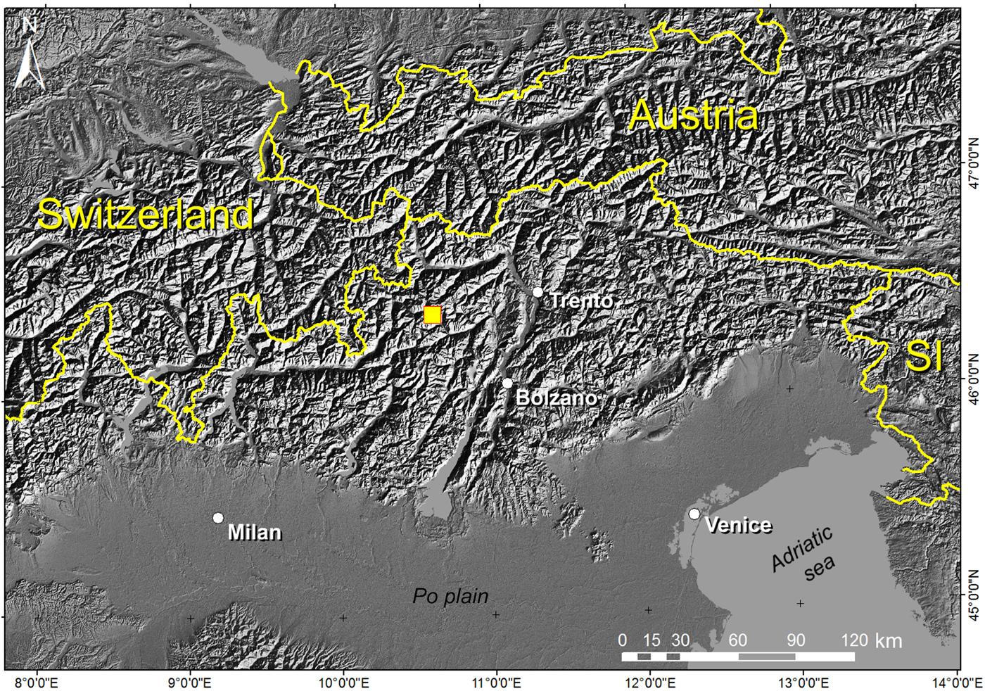
Fig. 1. Map of the Central Alps showing the study area.
The ice from the saddle flows northwards and splits into two tongues that feed both the Forni and the Vedretta Rossa glaciers. The two glaciers, which cover an area of ~12 km2 (Salvatore and others, Reference Salvatore2015), have been retreating since the end of the Little Ice Age of the mid of the XIX century (Pogliaghi, Reference Pogliaghi1883; Orombelli and Pelfini, Reference Orombelli and Pelfini1985). Analyses of historical photographs and glaciological reports (Baroni and others, Reference Baroni, Bondesan and Mortara2015, Reference Baroni, Bondesan and Mortara2016, Reference Baroni, Bondesan and Chiarle2017) have documented the reduction of the ice surface in the saddle area. Since WWI, the ice surface lowered of ~25–30 m and this has resulted in the exposure of several remains and military infrastructure.
During WWI, Punta Linke represented an important logistic emplacement and the highest advanced command of the Austrian Army (Francese and others, Reference Francese2015; Vergara and others, Reference Vergara, Bondesan and Ferrarese2017). The post was located just behind the front line, and it was part of a series of cableways connecting the nearby Pejo Valley to the Palon de La Mare glacier (Fig. 2) to transport supplies to higher altitudes. Cableways are still key elements in the supply chain for mountain huts and bivouacs at various Alpine sites. Punta Linke served as an intermediate station. Engines and warehouses were hosted inside a tunnel excavated in the rocks below Punta Linke. The entrance was built into the ice and some of the soldiers' barracks were located just outside. The station was connected to the rear lines via a network of surface routes and, probably, protected passages, including tunnels excavated in the rocks and in the glacier.
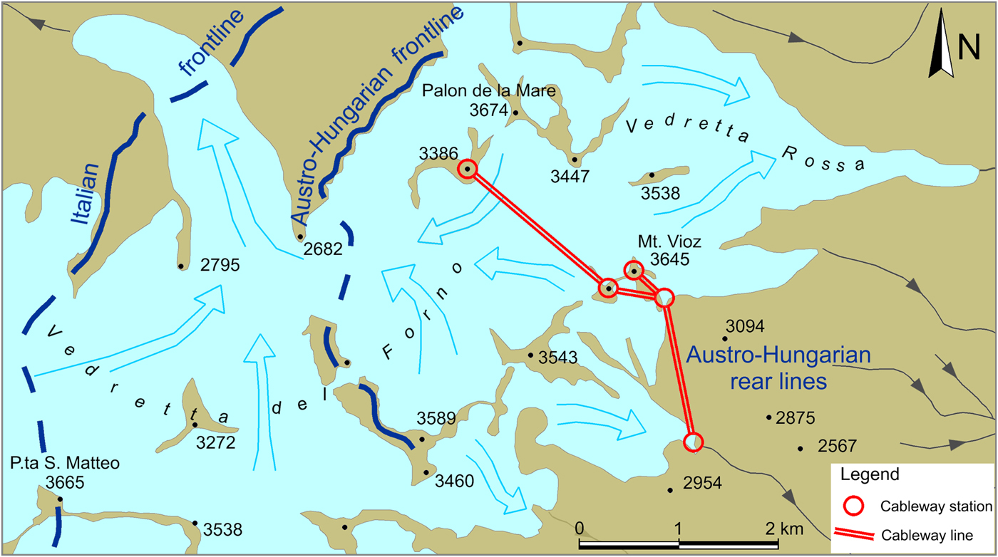
Fig. 2. Schematic map showing the frontline established in 1915 and the cableway system connecting Austro-Hungarian rear lines to the frontline.
The entrance to the tunnel on the south-east side of Punta Linke (Hill 3619) was on the protected side, shielded from Italian artillery fire. Sections of the cableway south of Monte Vioz were also sheltered from direct fire from the Italian artillery. The rock tunnel was built at the Punta Linke summit, outside the glacier at a height of at least +30 m. This was deduced from a comparison of the current glacier surface with historical photos from WWI. At this elevation, the thickness of the Punta Linke summit was limited, and the tunnel to be excavated in the rock was particularly short. The high altitude also favored the installation of the long cableway tract.
The connection between Monte Vioz and Punta Linke could be made on the surface of the glacier. Historical photographs (Österreichische Nationalbibliothek, 1917) illustrate a series of stakes that signed the footpath. According to oral testimony collected by the local inhabitants (Cappellozza Nicola, personal communication, 2011), the tunnels had been dug in the glacier to protect soldiers from adverse weather and Italian fire.
At the base of the glacial tongue extending along the south side of the saddle, a tunnel entrance consisting of a small stonewall still exists (Cappellozza Nicola, personal communication, 2011) even though the ice tunnel has disappeared with the retreat of the glacier.
Materials and methods
The site logistics were fairly complicated because transportation was possible by cargo helicopter only. Thus, the overall weight of the geophysical equipment that could be available on-site was limited.
Radar data were collected using a GSSI GPR equipped with antennas operating at 70 MHz (unshielded) and 200 MHz (shielded), corresponding to a nominal wavelength (λ) in Alpine ice of 2.1 m and 0.8 m respectively. The saddle area (Fig. 3) was covered with five profiles, collected during the 2010 campaign, and nine additional profiles collected during the 2011 campaign (Table 1). During the second campaign, 3 m-spaced profiles were collected parallel to the two axes of a 102 m × 51 m grid. Data were recorded in time domain, firing eight radar sweeps per second, and vertically stacking eight traces (Fig. 4). The average sweep spacing was 0.10 m in the stand-alone profiles and 0.05 m in the grid area. To achieve consistent coupling, both the two antennas were placed on a plastic sledge and towed along the surface. The record lengths were 600 ns for the 70 MHz dataset and 500 ns for the 200 MHz dataset.
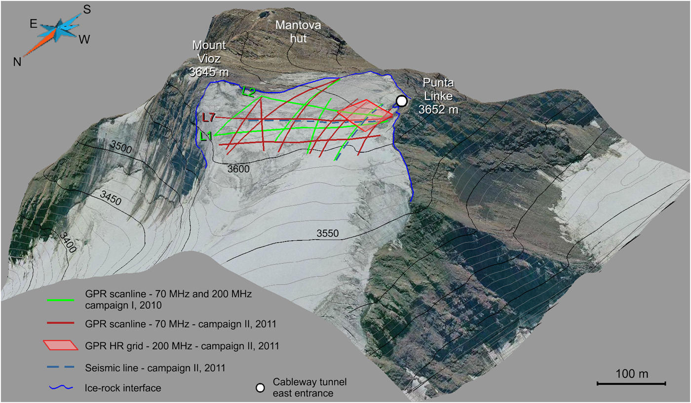
Fig. 3. Field layout during the 2010 and 2011 campaigns. The East entrance of the cableway station at Punta Linke is also indicated. The entrance is a tunnel excavated into the bedrock. The drapped image is a digital aerial image taken in 2003 by Regione Lombardia (released under common creative license CC-BY-NC-SA 3.0 Italy).
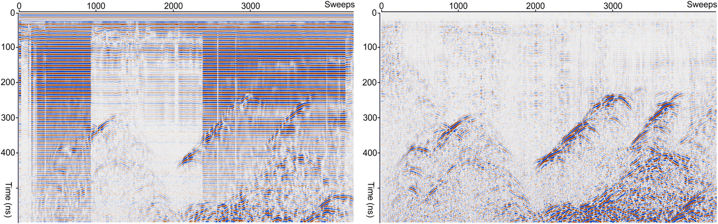
Fig. 4. Raw GPR record showing the superposition of two types of noise: horizontal bands and variable ringing (on the left). Processed record (on the right).
Table 1. Summary of geophysical survey

The theoretical resolution, based on the λ/8 criterion, was 0.25 m and 0.10 m for the 70 and 200 MHz antennas, respectively. For the real data, the resolution could be prudently estimated with the λ/4 approximation (Yilmaz, Reference Yilmaz2001).
Seismic data were collected using with a 24-channel Geometrics Geode seismograph during the summer 2011. Two lines were collected by the deployment of source and geophones along GPR profiles L7 and L3 (Table 1 and Fig. 3). Elastic energy was propagated in the subsurface with the use of an eight-caliber buffalo gun. Geophone spacing was set to 5.0 m, and the inline shots were recorded at each geophone station. In addition, several external shots were collected at positive and negative offsets. The incoming signal was detected with 4.5 Hz vertical geophones. The uppermost snow and firn porous layers made both the source and the receiver coupling quite difficult (Sen and others, Reference Sen1998). The recorded signal had a low amplitude and low frequency, particularly in the lower half of line L3a (Fig. 5).
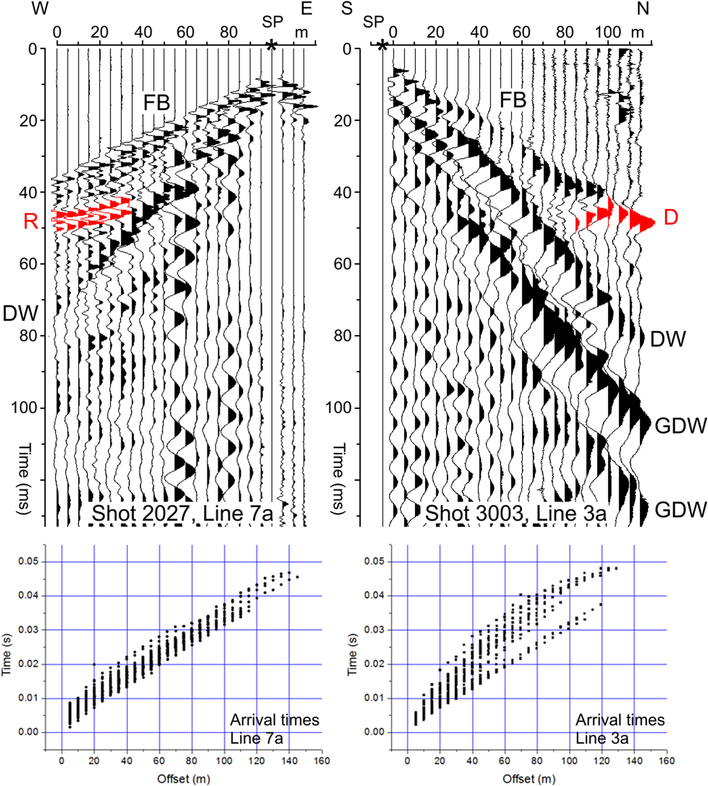
Fig. 5. Raw seismic records from line 7a - L7a (top left) and line 3a - L3a (top right). FB, first break; SP, shot point; DW, direct wave; GDW, guided direct wave; R, reflection; D, diffraction. Graphs showing first break versus offset along lines 7a (bottom left) and 3a (bottom right).
Positioning data were provided by means of geodetic GPS, in a differential configuration, operating in real-time kinematic (RTK) mode along with a standard total station. Some benchmark points were available near the summits of Mount Vioz and Punta Linke.
GPR data were processed in an open-source environment through the public domain software package Seismic Unix (Stockwell, Reference Stockwell1999; Cohen and Stockwell, Reference Cohen and Stockwell2011). The reflected signal was clearly visible from the near surface down to the later two-way traveltimes. The major processing steps included DC component removal, background removal (dewoving), zero offset correction to align the ground impact of each trace at time zero, bandpass filtering around the central frequency (cf) of the transducer (typically in the interval between cf/4 and 2 × cf), and finally, amplitude recovery to balance the amplitude decay caused by geometrical spreading and adsorption. A special effort was made to correct the differential elevation of the radar sweeps along the profile and to attenuate a spatially variant banding that overpowered the reflected signal in the 70 MHz datasets (Fig. 4). This noise appeared to be either coupling- or electronic-dependent (Seppi and others, Reference Seppi2015). The standard running average filter (Daniels, Reference Daniels1996; Francese and others, Reference Francese, Galgaro and Grespan2004) was not effective at removing these high-amplitude bands. An automatic routine was therefore coded for removing this specific noise. The scanline was split into subscans, each subscan was filtered with a running average approach and the filtered subscans were then combined back onto the original scanline (Fig. 4).
The last step was depth migration using the time-shift approach (Gadzag, Reference Gadzag1978). Although moving the reflectors to their true positions improved the resolution, the migration did not really increase the detectability of the ice inclusions. The diffraction hyperbola tails are often a major visual aid in mapping barely reflecting targets. The EM wave propagation velocity was estimated on the curvature of the most prominent hyperbola in the longitudinal scans of the grid dataset (Fig. 6). The optimum migration velocity was found to be ~0.160 m ns−1 corresponding to a relative dielectric constant of 3.5 (Fig. 7). A maximum error of 8–10% of the target depth (Fig. 7) was observed by comparing picking of the bedrock reflection on un-migrated and migrated data. As was expected, higher errors occurred where the bedrock was steeply dipping.

Fig. 6. Gadzag migration panel on data collected with a 200 MHz transducer, profile L110-2011, from the high-resolution grid of the 2011 campaign. (a) Unmigrated data; (b) migrated data using a Velocity (V) of 0.150 m ns−1: data are clearly undermigrated; (c) migrated data using a V of 0.160 m ns−1: data are just slightly overmigrated; (d) migrated data using a V of 0.175 m ns−1: data are significantly overmigrated.
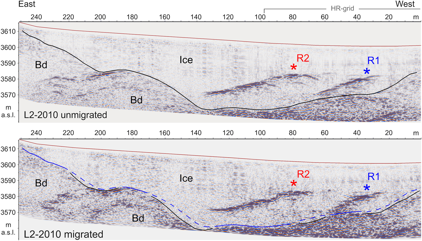
Fig. 7. GPR scanline L2-2010, collected with a 70 MHz transducer, before (top) and after migration (bottom). The bedrock reflection in the migrated section appears to be shifted downwards mostly where the bedrock is steeply dipping. Ice-embedded reflectors R1 and R2 are also outlined. Bd: bedrock (top image modified after Francese and others, Reference Francese2015).
Seismic data processing included geometry assignment, trace shifting to correct mis-triggering and bandpass filtering. The data quality was slightly different in the two profiles. First arrivals were clear and sharp in transversal line L7a (Fig. 5), also at larger offsets, while they were low amplitude, lower frequency and quite difficult to pick in the second half of the longitudinal line L3a. Furthermore, in line L3a, the direct wave (DW) was trapped in the uppermost water-saturated layer exhibiting a dispersive character (guided direct wave (GDW)) with its typical shingling effects (Robertsson and others, Reference Robertsson, Holliger, Green, Pugin and De Iaco1996). A total of 1250 first arrivals were picked in dataset L7a, and 600 first arrivals were picked in dataset L3a (Fig. 5). Bedrock internal reflections were also visible in the raw shots from line L7a but stacking these reflections was difficult. Some diffractions and lateral reflections, likely caused by crevasses, appear on line L3a at ~100 m of distance. The arrival times were converted into a velocity model via the classical diving-wave traveltime tomography approach (Böhm and others, Reference Böhm, Francese and Giorgi2010, Reference Böhm, Francese and Giorgi2012; Vesnaver, Reference Vesnaver2013). Inversion was performed with the Simultaneous Iterative Reconstruction Technique (SIRT) algorithm (Kak and Slaney, Reference Kak and Slaney1988). The misfit between real and calculated arrivals was very low for most of the rays. Cells initialized with velocity values but not crossed by rays were not considered in the interpretation.
Seismic data from line L7a were also analyzed to map reflectors. Processing was aimed at increasing the signal-to-noise ratio and improving the lateral coherency of the reflectors of interest and it was followed by an imaging procedure (Yilmaz, Reference Yilmaz2001). The sequence included: (1) bandpass filtering and trimmed-mean dynamic dip filtering (e.g. Giustiniani and others, Reference Giustiniani, Accaino, Picotti and Tinivella2008) to eliminate the random and coherent noise (GDW and DW); (2) predictive deconvolution for the wavelet compression; (3) amplitude recovery to compensate for geometrical spreading and adsorption; (4) stacking velocity analysis and (5) stacking (Picotti and others, Reference Picotti, Francese, Giorgi, Pettenati and Carcione2017). An iterative imaging procedure involving P-wave residual move-out analysis, traveltime tomography (Picotti and others, Reference Picotti, Vuan, Carcione, Horgan and Anandakrishnan2015) and prestack depth migration (Yilmaz, Reference Yilmaz2001; Picotti and others, Reference Picotti, Francese, Giorgi, Pettenati and Carcione2017) was used to generate a vertical seismic section of the glacier and of the underlying bedrock. The resulting interval velocity section was subsequently superimposed to the pre-stack depth migrated section.
Snow cover at the time of the survey was measured at various locations on the saddle. It was thinner than a few decimeters; thus, it was not considered in the data processing.
All the available GPR and seismic profiles were used in a 3D reconstruction of the bedrock morphology.
A digital terrain model (DTM) of the study area was constructed by merging high-resolution airborne laser data of the glacier surface (from a recent survey: Provincia Autonoma di Trento, 2008) and the digitized contour lines of the exposed rocks (from available cartography: Provincia Autonoma di Trento, 2008). These data were then interpolated over a 2.5 m aperture grid. DTM was then corrected with GPS measurements, taken at the time of the survey, to account for the yearly changes in the elevation of the glacier surface.
Results
GPR profiling allowed for a detailed reconstruction of bedrock reflectivity of the buried ice–rock interface and subsequently of several ice-embedded structures.
Bedrock reflectivity
Bedrock signature was visible in a majority of the profiles in the two-way traveltime window. The bedrock was out of GPR range in the lower slope, close to the end of the longitudinal profiles, where the glacier thickens (Fig. 8). This signature was less sharp than expected (Carturan and others, Reference Carturan2013) as it appears to be a composite reflector rather than a unique event. The reflection character was more consistent where the bedrock is gently dipping; however, it is rather complex elsewhere. Some 3D effects caused by abrupt changes in the bedrock morphology were also observed in the collected profiles.
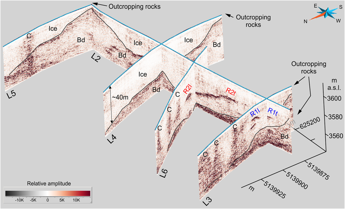
Fig. 8. Three-dimensional view of GPR scanlines L2, L3, L4, L5 and L6 collected with a 70 MHz transducer during the 2010 campaign. The bedrock reflection at the intersections shows no apparent vertical shifts, thereby indicating the consistent EM response of the longitudinal and transversal profiles. The ice layer appears to be almost transparent to the 70 MHz wavelet, and the bedrock exhibits several internal reflections. The R1 and R2 ice-embedded reflectors which were imaged longitudinally (l) and transversally (t), are also outlined. Bd: bedrock, C: crevasse.
Bedrock morphology and glacier thickness
Outcropping rocks were the key to interpret the GPR profiles because they provided robust constraints in the recognition of the bedrock signature and in the lateral correlation of this reflection along the entire profile (Fig. 8).
The bedrock is steeply dipping in the upper part of the saddle and on the saddle flanks. Its inclination near Punta Linke and Mount Vioz could be as much as 40°. It reduces to 10–15° along the slope. The bedrock geometry is clearly undulated with two elongated longitudinal mounds (marked ‘b’ and ‘c’ in Fig. 9) and a transversal ridge (marked ‘d’ in Fig. 9). The eastern mound could be inferred by an analysis of the curved geometry of the crevasses. This geometry is indicative of shallower bedrock.
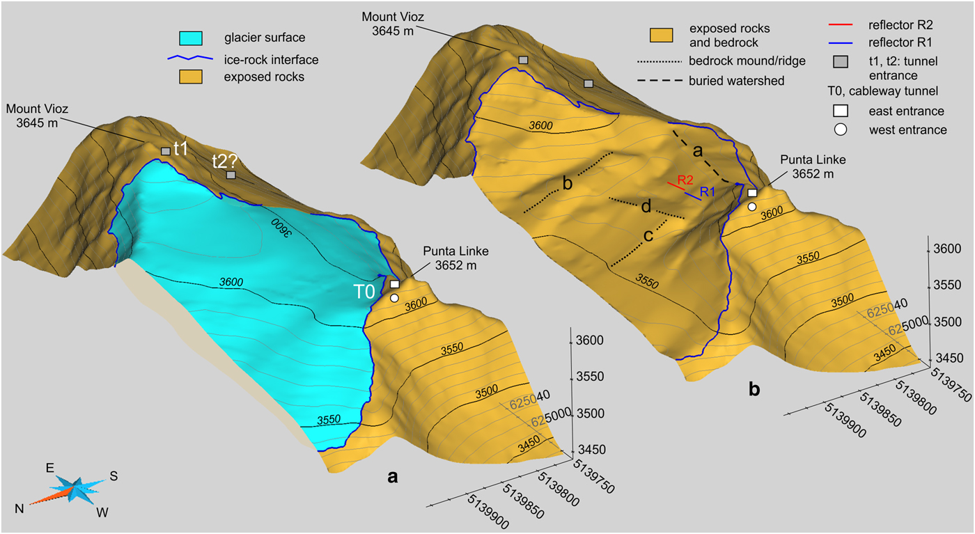
Fig. 9. Comprehensive 3D view of visible (a) and buried (b) morphology. Bedrock undulations and ridges (marked ‘b’, ‘c’ and ‘d’) are clearly visible in the reconstructed bedrock morphology. The buried water-divide (marked ‘a’) is also visible. Reflectors R1 and R2, as well as the cableway station entrances (T0), below Punta Linke are outlined; t1 and t2 are recently discovered tunnel entrances that could be related to the cableway system and the anomalous reflectors R1 and R2 in the glacier body.
A buried watershed (marked ‘a’ in Fig. 9) is located just south of the ice-divide. This buried watershed appears to be shifted ~50 m from the vertical projection of the ice-divide (Fig. 9). The ice-divide could have been also shifted because its position is controlled by snowdrifting under wind control, but at the time of the survey, there was just a patchy snow cover. The ice surface watershed was then precisely surveyed by GPS.
The reliability of the ice thickness assessment was evaluated at the profile intersections. The thickness difference was marginal and <2% based on the data collected in the same campaign; however, it was moderately higher and ~3–4%, comparing GPR data collected in the two campaigns. These differences between the 2010 and the 2011 campaigns resulted mostly from the varying water content that affected the EM velocity. The higher temperature during the 2011 campaign was the cause of some small melting water ponds at various locations along the GPR profiles.
A medium-resolution triangulated surface was turned into a regular grid (2.5 m × 2.5 m) through the standard kriging approach. The maximum thickness of the glacier in the investigated area, near the northeast corner of the slope, was 50 ± 1 m (Fig. 10). Surface observations on the exposures confirmed this estimate. The most depressed zones in the bedrock are elongated in the longitudinal direction and separated by the two previously mentioned mounds. The ice volume could be estimated at 2.24 × 10+6 ± 3.45 × 10+5 cubic meters. This value can be used as a reference for future mass-balance calculations.
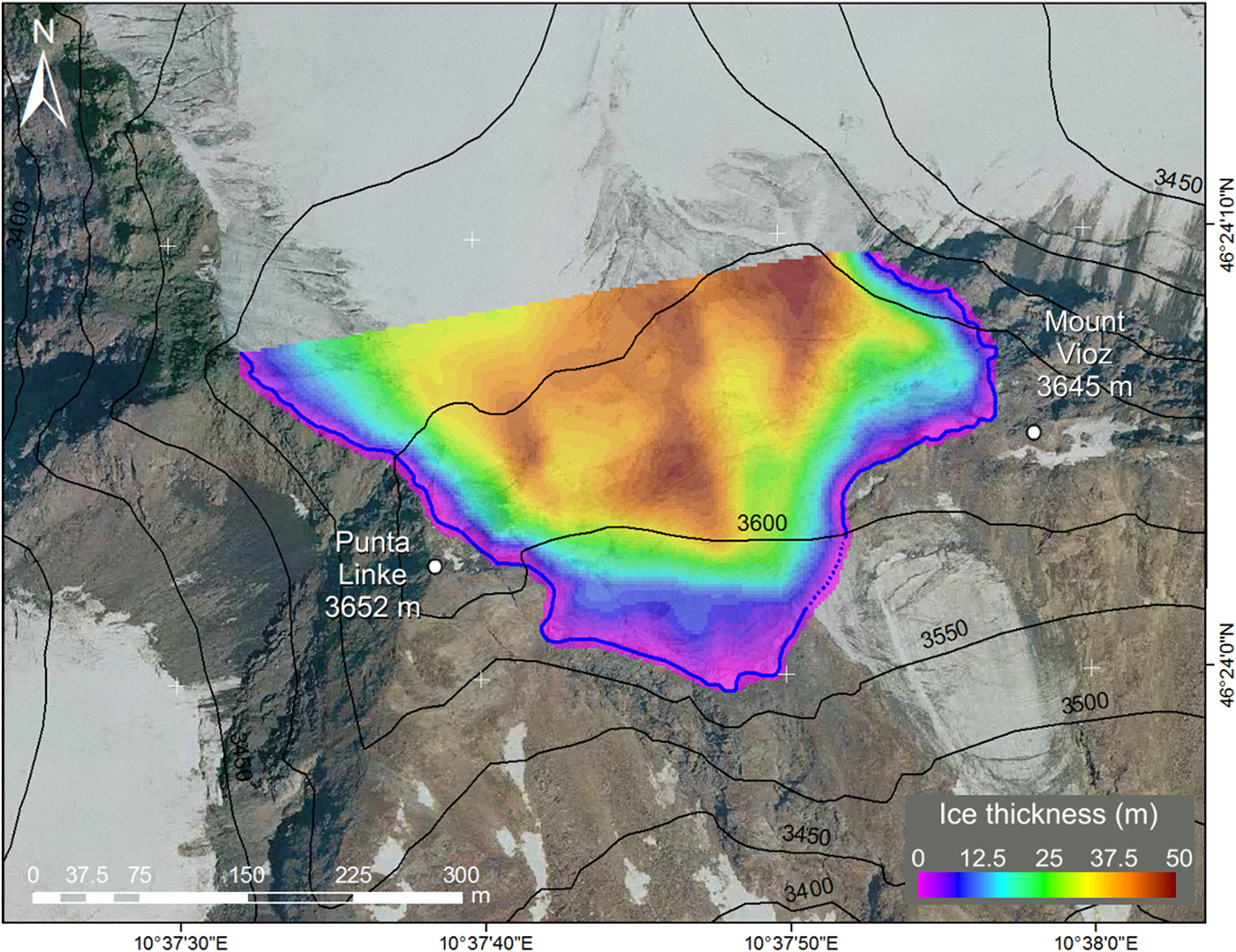
Fig. 10. Interpolated ice thickness with ice–bedrock interface blue line. The western bedrock ridge (marked ‘b’ in Fig. 9) is fairly visible as a relative minimum in the ice thickness. The eastern ridge is also visible (marked ‘c’ in Fig. 9). Because of its complicated morphology and the proximity of a longitudinal ridge, the eastern ridge is still detectable, but it is not very clear in the ice thickness map. The background is a digital aerial image taken in 2003 by Regione Lombardia (released under common creative license: CC-BY-NC-SA 3.0 Italy).
Seismic data provided insight into the properties and thickness of the glacier ice. The compressional wave velocity (V P) ranges from 800 to 3800 m s−1. The velocity model is slightly different in the transversal and longitudinal profiles. V P in the very near surface layer appears to be strongly controlled by the high water content. Its average value, 1500 m s−1, is almost coincident with the typical velocity of compressional waves in water. In the underlying ice body, V P gradually increases up to 3800 m s−1. The transversal profile L7a is mostly homogeneous and V P increases with depth despite the three zones of clear minima (LVZ in Figs 11, 12).
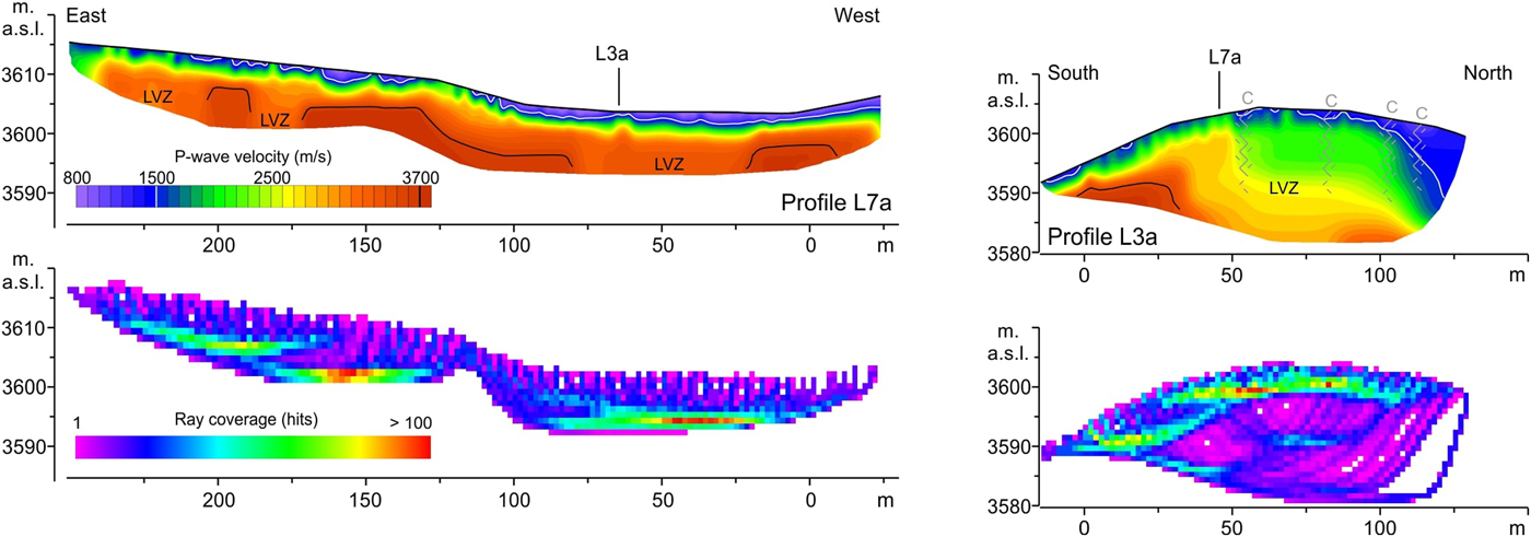
Fig. 11. Diving-wave seismic tomography section along profiles L7a (top left) and L3a (top right). The ray coverage maps for the two profiles are displayed at the bottom. The black line marks the 3700 m s−1 contour line. LVZ, low velocity zone; C, crevasse. See text for description.
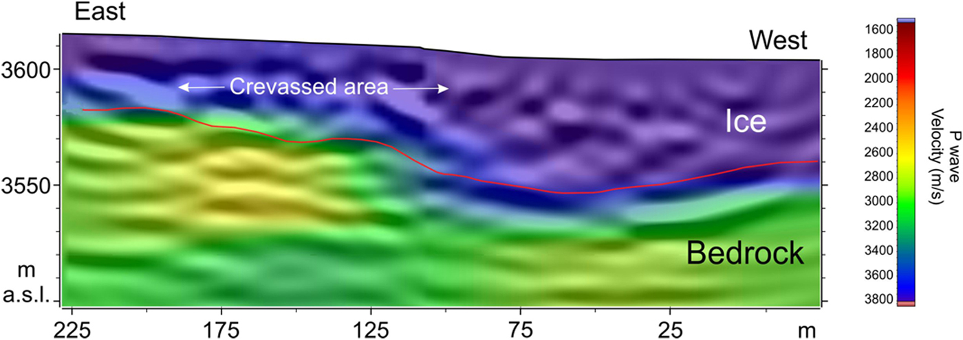
Fig. 12. Seismic reflection migrated section along profile L3a. The ice–bedrock interface, which was too deep to be detected with the sole diving-wave seismic tomography approach (Fig. 11), is a sharp reflector on mostly the western side of the profile where this interface is deeper. The interface is clearly undulated, and its depth correlates nicely with the GPR data. The velocity map in the background shows a low-velocity zone caused by the crevasses.
GPR profiling indicates that seismic profile L7a did not intersect important crevasses. The minima could be correlated to the presence of abundant melting water. Two of these minima correspond to the zones of the curved reflectors in GPR profile L1 (Fig. 13). Profile L1 is almost parallel to the seismic profile L7a and it is far away at 13 m. On the basis of the available results, whether the curved reflectors were caused by normal ice gravity or whether they were the result of a collapse is unclear.
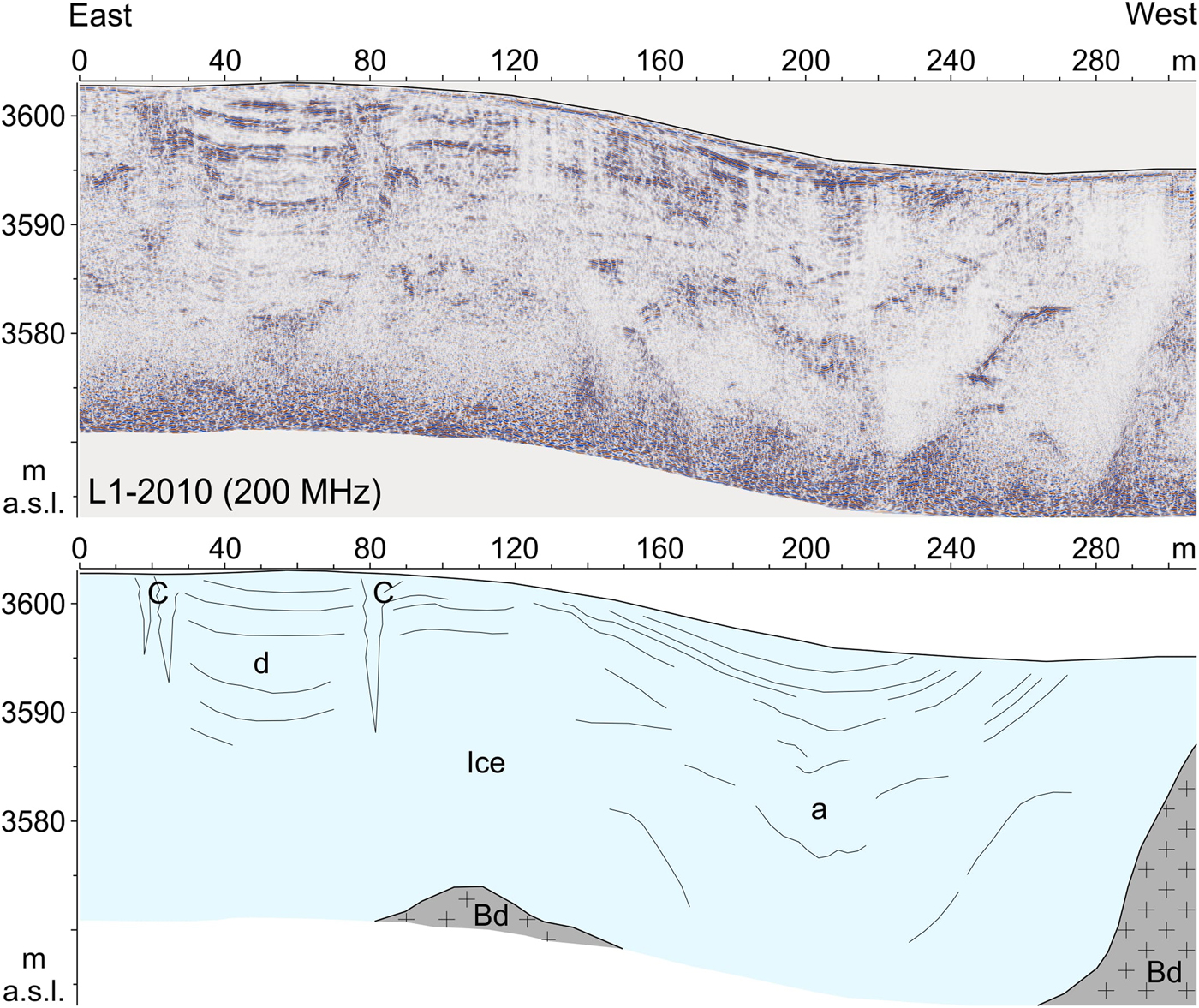
Fig. 13. GPR scanline L1-2010 collected with a 200 MHz transducer: processed data (top) and interpretation (bottom). The ice layer appears to be quite reflective, and some curved reflectors (marked ‘a’ and ‘d’), as well as some crevasses (marked ‘C’) with their typical diffraction patterns, are clearly imaged. The curved reflectors correspond to the zones of minima in the V P velocity maps. Bd, bedrock; C, crevasse. See text for description.
The longitudinal profile L3a is quite anomalous because northern of the intersection with profile L7a V P drops down to values not compatible with glacier ice. This is caused by the presence of a series of subparallel air- and water-filled crevasses. The crevasses are clearly visible in GPR profile L3 (Fig. 8). Because of the large number of crevasses, the V P field in this segment of the profile is strongly biased; thus the velocity values could not be used as reliable indicators of the ice properties.
Seismic depth migrated (Fig. 12), although slightly noisy, outlined the bedrock reflection below radar range in the southern portion of the glacier. According to the GPR results, the bedrock morphology appears to be concave, showing a minimum on the western side of the profile and increasing its elevation toward the east. Reflection tomography provided further insight into the velocity field. V P in the ice is ~3800 m s−1, and in the underlying bedrock, it ranges from 2700 m s−1 to values larger than 3200 m s−1. V P in the ice body exhibits some minima in the x-interval 100–200 m. The reason might be the presence of crevasses. This is partly confirmed by the traveltime tomography analysis. Bedrock velocity also shows slight variations with several minima along the profile. This could be caused by fractures or, more likely, the presence of water and sediments. Unfortunately, a thin low-velocity layer (comprised of water and/or sediment) on top of the bedrock is outside the resolution capability of the stacked signals. Some difficulties that arose while the seismic source was being coupled resulted in a slightly narrow signal bandwidth (~100 Hz); thus, the resolution was limited.
Ice-embedded structures
A comprehensive understanding of the bedrock morphology and the overall ice properties was needed for interpreting many types of ice-embedded reflectors visible in the GPR data. A series of complicate reflection/diffraction patterns (marked ‘C’ in figures) caused by the crevasses appear as prominent features. These events exhibit a typical character, with repeated diffractions along a narrow vertical stripe of the profile (Figs 8, 13). Aerial photos taken during late summer (Fig. 10) confirmed the presence of a crevasse at each of these reflecting spots. Additional features resulted in a group of curved and weak reflectors (marked ‘a’ and ‘d’ in Fig. 13). These reflectors, which likely represent seasonal ice layering, define two distinct concave shapes in the 200 MHz dataset (Fig. 13) while they are barely visible in the 70 MHz profiles. It is worth nothing that the ice flow dynamic in the glacier saddle is supposed to be marginal and the expected ice folding should have occurred along an east-west axis. The concave structure, visible on the east side of the profile (marked ‘d’) and enclosed by crevasses, indicates a minor depression which could have been caused by the local circulation of melting water or the normal ice flow dynamic. On the contrary, the concave structure located on the west side of the profile (marked ‘a’) is larger and anomalous and appears to have been caused by the collapse of the underlying ice strata.
Finally, clearly visible in the GPR profiles are a series of high-amplitude and sharp reflections located right in the middle of the ice body and unrelated to the glacier surface or the crevasses (marked ‘R1’ and ‘R2’). These features, initially mapped in the 2010 campaign (Figs 7, 8) and further investigated in 2011 (Fig. 14), exhibit a classic diffraction hyperbola generally caused by buried pipes. The radar signature is fairly consistent for the sparse profiles (Figs 7, 8) and the rectangular grid (Fig. 14). In addition, the curvature of the hyperbolas is homogeneous. This suggests a regular shape of the reflector and the presence of minor lateral changes in the EM wave velocity.

Fig. 14. Three-dimensional view of GPR scanlines L112, L206, L218 and T301 collected with a 200 MHz transducer, on the high-resolution grid during the 2011 campaign. To ensure clarity the other scanlines are not displayed. The interpreted ice–bedrock interface is represented as a grey surface. Ice-embedded reflectors R1 and R2 are clearly visible and could be easily correlated across the different scanlines.
Modeling
EM wave propagation modeling was utilized to constrain the interpretation. The radargrams were computed in the space–time domain. Propagation in the (x, z)-plane was assumed. It was also assumed that the material properties and source characteristics were constant with respect to the y-coordinate. The corresponding time-domain electric and magnetic fields and sources were denoted by ${\rm {\cal E}}$ and ${\rm {\cal H}}$
 and ${\rm {\cal J}}$
 and ${\rm {\cal M}}$
 . Under these conditions, Ex, Ez and Hy were decoupled from Ey, Hx and Hz, and the first three fields obey the TM wave differential equations:


The set of properties μ, ε and σ denote magnetic permeability, dielectric permittivity and electrical conductivity, respectively. The first was assumed to be the vacuum value. The numerical solver used here consisted of the pseudospectral Fourier method for computing the spatial derivatives and a Runge–Kutta method for time integration (Carcione, Reference Carcione1996a, Reference Carcione1996b, Reference Carcione2015).
Synthetic GPR data have been generated in a variety of subsurface scenarios to provide adequate insight to assist data interpretation. The anomalous reflector exhibits a sharp and consistent signature while moving to different scanlines (Fig. 14). The wavelet character is approximately the same on a long segment of the reflector, both for amplitude and bandwidth, thus suggesting the artificial nature of the ice-embedded target.
The numerical mesh for the plane-wave simulations has 675 × 675 grid points, with a grid spacing of 0.1 m. The model is shown in Figure 15a. The first five grid points at the top represent an air layer. Five model scenarios were considered:
(1) Decauville horizontal track (10 cm × 10 cm) separated by 1 m (Fig. 15b);
(2) Decauville vertical track (10 cm × 10 cm) separated by 1 m (Fig. 15c);
(3) Square tunnel sized 2 m × 2 m filled with air (Fig. 15d);
(4) Round tunnel (1 m radius) filled with air (Fig. 15e);
(5) Round tunnel (1 m radius) filled with air and 50 cm water (Fig. 15f).
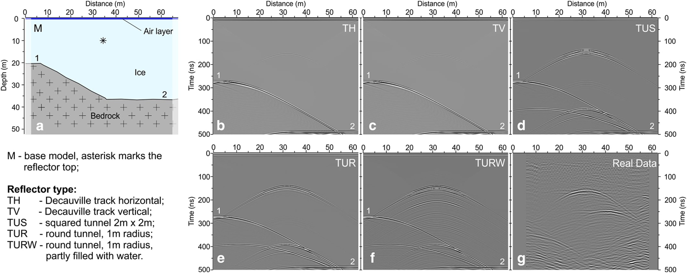
Fig. 15. Results from numerical modeling. M: subsurface model (a); TH: response from a Decauville railway with horizontal track (b); TV: response from a Decauville railway with vertical track (c); TUS: response from a squared tunnel 2 m × 2 m (d); TUR: response from a round tunnel with a 1 m radius (e); TURW: response from a round tunnel with a 1 m radius partly filled with water (f); real data (g). See text for comments.
The model properties are visible in Table 2. Zeng and West (Reference Zeng and West1996) smoothing method was used to damp the diffractions resulting from the discretization of the model. The source was horizontal electric current plane-wave (${\rm {\cal J}}x$ ), whose time history is a Ricker wavelet with a central frequency of 200 MHz (e.g. Carcione, Reference Carcione1996a, Reference Carcione1996b). To avoid wraparound, absorbing layers 20 grid points in length were implemented at the sides of the numerical mesh, with the upper absorbing layer located at the bottom of the mesh, given that the Fourier differentiation is periodic. The Runge–Kutta method required a time step of 0.2 ns.
Table 2. Electromagnetic properties used for numerical modeling

Permittivity of free space: ε 0 = 8.854·10−12 F m−1.
The Decauville railway has been considered, as it was commonly used for moving goods and ammunition to different locations along the WWI frontline in the Alps (Klebelsberg, Reference Klebelsberg1920; Bertarelli, Reference Bertarelli1923). This small railway was later used in 1930 for the Maginot defense line in the French Alps. Case #1 (Fig. 15b) simulates the response of a horizontal track. The reflection has a very low amplitude and it appears as a single reflector with short hyperbola tails. The bedrock reflection has a much higher amplitude. The wavelet character and the ringing patterns are slightly different from those of the real case (Fig. 15g). Case #2 still considers a Decauville railway, but the track was positioned vertically (Fig. 15c). It is a limit case because it was assumed that over the past century, the ice had moved several meters, curving the track and crushing the wooden ties. This reflection has very low amplitude, with short hyperbola tails, although it exhibits more reverberations than were seen in case #1. The vertical track response compares poorly to that of the real data. Case #3 considers a square tunnel that was 2 m on each side (Fig. 15d). The reflection appears to be composite given the complicated interferences between the top and bottom back-scattering and corner diffractions. The amplitude is comparable to that of the underlying bedrock reflection. A multiple reflection is clearly visible at ~400 ns. The wavelet character, hyperbola tails and ringing patterns are somewhat similar to those in the real data, although the real reflector is smoother and does not exhibit such interferences. Case #4 simulates an air-filled tunnel of 1 m radius (Fig. 15e). Reflection is sharp with long hyperbola tails and a typical ringy character. It is a wavetrain comprising a primary and two cycles of reverberations. The amplitude is comparable to bedrock reflection. A multiple reflection is clearly visible at 400 ns of two-way traveltime. This simulation compares well to the real data. Case #5 (Fig. 15f) is the last modeled. It simulates a tunnel of 1 m radius partly filled with water. The primary reflection is sharp, as with case #4, with long hyperbola tails; however, the reverberations appear organized in multiple cycles, and they superimpose on the first multiple. In terms of the wavelet character and reverberation patterns, this case is probably the most similar to the real data.
Discussion
Electro-magnetic and compressional wave velocity
An EM wave velocity of 0.160 m ns−1 could be considered somewhat low compared to the value of 0.168 m ns−1 that is typical for cold ice (Bradford and others, Reference Bradford, Nichols, Mikesell and Harper2009; Garambois and others, Reference Garambois, Legchenko, Vincent and Thibert2016). The presence of melting water (Bradford and others, Reference Bradford, Nichols, Mikesell and Harper2009) is likely the primary factor affecting EM velocity. Other factors are voids and the debris embedded in the glacier. Alpine glaciers in the Alps are polythermal; thus, they could be considered cold above an elevation of 3500 m (Garambois and others, Reference Garambois, Legchenko, Vincent and Thibert2016). According to Haeberli and others (Reference Haeberli, Frauenfelder, Kääb and Wagner2004), with an annual average temperature at −10 m of −4°C, there is no basal sliding. In such conditions, the movement at the base ice body (ice/bedrock interface) may be close to zero and the age of basal ice layers may be considerable (historical, Holocene or even last ice age). The yearly average temperature recorded at the nearby site of the Careser dam is −1°C. Considering the denivelation between Punta Linke (3632 m a.s.l.) and Careser Dam (2603 m a.s.l.) and the vertical thermal gradient (~0.65°C every 100 m), the annual average temperature at Mount Vioz-Punta Linke could be estimated at ~−7°C. The low or absent sliding hypothesis could be also supported in the absence of any evidence of Bergschrund on the saddle flanks.
In reality, thermal conditions depend on a variety of factors, and only thin parts probably remain cold (Eisen and others, Reference Eisen, Bauder, Lüthi, Riesen and Funk2009). The value of 0.160 m ns−1 could then be consistent with a condition of partly melting ice. Melting water was observed at the surface at survey time during the 2011 campaign.
V P is also lower than that of other glaciers (Horgan and others, Reference Horgan2012) and also of the nearby Mandrone Glacier (Picotti and others, Reference Picotti, Francese, Giorgi, Pettenati and Carcione2017) located in the Adamello massif. However, low V P are not uncommon in temperate glaciers (Navarro and others, Reference Navarro, Macheret and Benjumea2005) where the presence of melting water could affect the velocity of the elastic waves and cause their values to be significantly lower.
Bedrock reflectivity
The amplitude of the reflected EM waves was strictly controlled by the shape and inclination of the bedrock shape. Moreover, the presence of fine debris and water also affects the total amount of backscattered energy. Conductive debris rich in clay minerals (e.g. micas) is often present in crystalline rocks. It causes dispersion. In some cases, the debris layer could be thick enough to attenuate the radar waves (Carturan and others, Reference Carturan2013). The antenna footprint of the low- and medium-frequency transducers is more or less an ellipse elongated perpendicularly to the major axis of the transmitting dipole. The 70 and 200 MHz antennas were dragged with different dipole orientations. In the 70 MHz dataset, the long axis of the dipole was parallel to the profile, while in the 200 MHz dataset, the scanning direction was perpendicular to the major axis of the dipole.
This difference in the setup affected the amplitude responses. This is particularly true with the 70 MHz dataset because of its larger footprint. In the longitudinal profile, the dipping bedrock caused a significant amount of energy to back scatter outside the receiving fan of the transducer (Forte and others, Reference Forte, Pipan, Francese and Godio2015). This occurrence is more evident in the areas with steeply dipping bedrock that are typically located near the edge of the glacier. This dependence of the reflectivity with respect to footprint orientation reduces the possibility of a robust correlation between the longitudinal and transversal profiles. Mapping the interface in the vicinity of the glacier edge would have therefore been more efficient than dragging the antennas parallel to the bedrock contours. The bedrock inclination at larger depths (i.e. more than 15–20 m) is less pronounced, thereby making the transversal and longitudinal responses more comparable.
Glaciological notes
The reconstruction performed through the interpolation of the GPR reflectors allowed for the definition of the morphology of the bedrock surface. At the bottom of the glacier were also observed some rocky ridges (marked ‘a’, ‘b’, ‘c’ and ‘d’ in Fig. 9) that are likely connected to more resistant sectors of the rock or to structural features.
The GPR section of Figure 13 shows the typical concave reflectors that can be interpreted as the layers of ice, which gradually accumulated during the glacier growth phase and were therefore involved in the downward glacial flow. For this reason, the arched shape has been preserved.
The entire glacial mass was subjected to very limited movement. This can be inferred from the poor deformation of the ice layers and the stability of the crevasses that also retained the same shape and position over the years (this can be inferred from the comparison between the aerial photography from 2003 and of the radar survey from 2011). In addition, the large amount of war material (shells, wooden boxes, tools, equipment, etc.) scattered around the access shack to the cableway tunnel does not exhibit, after a century, evidence of translational movements of the glacial surface. These materials scattered when the Austro-Hungarians exploded the ammunition deposits at the end of the conflict.
Ice-embedded structures
Glaciological considerations regarding the ice flow dynamics associated with the geophysical reconstruction of the ice–bedrock interface in the saddle and in the upper slope defined the framework for the interpretation of the ice-embedded structures imaged by GPR and Seismic.
The crevasses show a typical geophysical response as they cause the scattering of EM waves and the lowering of elastic wave velocities. The horizontal position could be easily mapped in the GPR scanlines and their depths could be inferred by analyses of V P maps in specific low-velocity zones.
The high-amplitude reflector located in the saddle could be associated with several targets. The authors are aware of the difficulties in supporting the uniqueness of any interpretation. Englacial structures, such as cavities, sediment and boulders are quite common in glaciers (Murray and Booth, Reference Murray and Booth2010). The shape of the reflector, the wavelet character and the consistency of its signature indicate the presence of either a glacial conduit/cavity or a tunnel excavated during WWI. The origin of the target is different, but its morphology and features are somewhat similar. A tunnel is generally straighter and more regular. In contrast, a glacial conduit or cavity has a crooked pattern and is generally irregular in section and morphology (Garambois and others, Reference Garambois, Legchenko, Vincent and Thibert2016). Results from the modeling showed how the case of a 1 m round void partly filled with water could better fit the real data. The additional presence of a Decauville track in the void, almost parallel to the surface, could not be completely excluded. Simulations indicate how, at the modeled depth, the track is a weak reflector when compared with the top and bottom reflections caused by the void in the ice.
The discussion about artificial (tunnel) versus natural (glacial conduit) could add some extra elements to support a more robust interpretation.
The tunnel hypothesis could be supported by several considerations.
(a) The direction of the tunnel is exactly as expected in this theater of war. The tunnel links the Punta Linke cableway with the Mount Vioz cableway and the Mantova hut rear lines.
(b) The direction of the tunnel is consistent with some of the entrances recently discovered after the glacial retreat near the Mantova hut (Fig. 9).
(c) The tunnel in the GPR profiles appears to be broken in two segments (R1 and R2 in Fig. 9 and Fig. 14). A glacial conduit should have appeared as a continuous structure, and the dip should have been consistent with the slope.
(d) Surface water was not entering any moulin, nor were the vertical shafts absorbing the melting water. The surface water circulation in the saddle is just marginal.
(e) A glacial conduit is a feature specific to the very lower part of the glacier close to the terminus where several glacial mills can be seen. Channelized water was not found in the saddle.
(f) The saddle elevation is ~3600 m a.s.l. and there is no catchment above the saddle to collect the runoff and/or melting water that is creating the underground circulation.
(g) The tunnel is elongated and is almost parallel to the elevation contour; however, a conduit is supposed to intersect the elevation contours at medium and high angles.
(h) Englacial conduits are rarely described in the upper portion of a glacier, and, as was previously mentioned, these conduits are transversal rather than longitudinal.
Tunnels excavated in ice were quite common during WWI in similar glacio-morphological settings and in some nearby glaciers (e.g. Zebru glacier in the Ortler massif). These tunnels also had Decauville tracks (Bertarelli, Reference Bertarelli1923). A total of 11.5 km of ice tunnels were excavated just in the Ortler group (Bertarelli, Reference Bertarelli1923). Some tunnels were also excavated at lower elevations (e.g. the Ice City in the Marmolada glacier). In a few cases, the tunnels had reached down to the underlying bedrock (Handl, Reference Handl1916, Reference Handl1917).
The glacial conduit hypothesis could be supported mostly by modeling results and by the recent climatic changes:
(a) The GPR simulations from a partly water-filled conduit (Fig. 15f) appear to be very similar to the real data. The presence of water caused severe reverberations in the GPR response. These types of patterns are visible on the scanlines collected on the top of the conduit.
(b) Ice melting over the last years has produced a significant amount of water. This supports the thesis of the presence of an englacial channel in the glacier body.
Finally, a tunnel excavated in the ice in 1918 is not expected to be still open after more than 90 years unless other phenomena (e.g. water circulation or very slow movement) were involved.
In sum, all of the above considerations lead to an attempt at a comprehensive hypothesis:
(a) The tunnel did not close because of the limited amount of ice movement in the saddle. The minimal amount of movement is confirmed by the enormous amount of WWI remains visible in the saddle just below Punta Linke. At the end of WWI, military supplies and ammunition were destroyed by an explosion, and the debris was scattered on the ice surface. Today, the debris appears to be more in approximately the same position. The maximum movement of the ice generally occurs in the uppermost layers. If the near surface layers moved just marginally, the deeper ice layer probably did not move at all.
(b) The melting water partly reactivated the tunnel as a glacial conduit. The water moved vertically along the crevasses and subsequently drained off along the tunnel. The presence of water in the tunnel is a further reason for the preservation of the tunnel itself because water flow caused partial ice melting inside the tunnel.
The reason for the preservation of the tunnel is therefore twofold: marginal ice movement and partial ice melting caused by the water flow in the tunnel. The tunnel size as estimated by reflection hyperbola in real data is smaller in diameter than the one modeled in numerical simulations (whose diameter of 2.0 m is comparable to other tunnels excavated in the ice during WWI). Since the end of the war, these tunnels, due to glacial pressure (Bondesan and others, Reference Bondesan, Carton and Laterza2015), progressively reduced their diameter.
The joint analysis of the newly collected geophysical data and the available historical data indicates the likelihood of a preserved WWI tunnel located in the saddle between Punta Linke and Mount Vioz.
Conclusions
During WWI, Mount Vioz and Punta Linke needed to be connected for the movement of supplies and ammunition through the cableway from the rear lines to the frontline. Photographs taken during the war clearly show a footpath on the glacier saddle. However, oral testimony and documents related to the nearby glaciers suggest the presence of a tunnel, probably with a built-in Decauville railway.
GPR and seismic profiles collected in the WWI scenario of the glacier saddle between Punta Linke and Mount Vioz, in the Ortler-Cevedeale massif, allowed for the reconstruction of glacier geometry and properties and anomalous ice-embedded structures likely related to WWI.
The values for EM and P-wave velocity were lower than those of other glaciers in the Alps: 0.16 m ns−1 and 3500 m s−1, respectively. These moderately low values are related mostly to the presence of melting water (EM velocity and V P) and the crevasses (V P). EM bedrock reflectivity appears to be highly dependent on antenna orientation, especially at depths below 15–20 m. The bedrock morphology was reconstructed through the integration of GPR and seismic data. The bedrock appears to be rather complicated with two elongated parallel ridges in the dipping direction. The maximum ice thickness in the investigated area is ~50 m just north of the saddle. The subsurface water-divide is shifted southwards compared to the surface topography and the ice-divide. This was caused by retrogressive glacial erosion that enlarged the valley head. The Bergschrund is located farther downstream from the ice-divide.
The most controversial feature in the englacial reflectors is a linear structure, split into two moderately dipping segments, ~120 m in length. The reflected wavelet character is fairly consistent in the various scanlines. This indicates the artificial nature of the reflector. Modeling of the EM wave propagation was used to support this interpretation. Numerical simulations constrained the interpretation to basic feature geometry and reduced uncertainty. The model that seems to better fit the real data is a cylindrical cavity of ~1 m in radius partly filled with water. The cavity could be interpreted either as a tunnel or a glacial conduit. Careful analysis of the pro and contra elements indicates how a tunnel partly reactivated as a glacial conduit could be the most satisfying hypothesis. The simulation results could not confirm or exclude the presence of a Decauville track because its weak reflection is overpowered by the top and bottom reflections from the tunnel and by the associated multiples. Should this interpretation be confirmed, it would be the first discovery of a preserved WWI ice tunnel. Borehole investigations could resolve the ambiguity; however, the target depth and site elevation require professional equipment and complex logistics to achieve this goal. Such research is not yet planned.
Acknowledgements
The research was conducted in the framework of the project ‘The glaciological context of the Great War site of Punta Linke (Ortles-Cevedale Group)’ conducted by the Italian Glaciological Committee (scientific coordinator Carlo Baroni) in collaboration with the Provincia di Trento – Soprintendenza per i Beni Librari, Archivistici e Archeologici – Settore Beni Archeologici (scientific coordinator Franco Nicolis). The project was funded by the Province of Trento, by the National Institute of Oceanography and of Experimental Geophysics – OGS of Trieste and by the University of Padova. We gratefully acknowledge Adastra Engineering s.r.l. for providing part of the geophysical and topographic equipment used in the project.
Author contribution
Roberto Francese, Massimo Giorgi and Aldino Bondesan designed the survey. Massimo Giorgi, Aldino Bondesan, Carlo Baroni and Maria Cristina Salvatore collected the geophysical data during the 2010 and 2011 campaigns. Roberto Francese, Stefano Picotti and Massimo Giorgi processed the geophysical data. José M. Carcione carried out the modeling. All authors have given substantial contributions to the interpretations of the data and the writing of the article. All authors approve of the submitted version of the manuscript and thereby agree to be accountable for all aspects of the work, ensuring that questions related to the accuracy or integrity of any part of the work are appropriately investigated and resolved.
Conflict of interest
The authors declare that the research was conducted in the absence of any commercial or financial relationships that could be construed as a potential conflict of interest.


 Open access