


Introduction
Glaciers distinct from the Antarctic and Greenland ice sheets are one of the key elements of the cryosphere and are major freshwater reservoirs (Millan and others, Reference Millan, Mouginot, Rabatel and Morlighem2022). As a result of climate change, these large freshwater stores are now melting at a fast rate, increasing global sea levels (Zemp and others, Reference Zemp2019; Hugonnet and others, Reference Hugonnet2021). After thermal expansion, glaciers and ice sheets are the largest contributors to sea-level rise in the 21st century (IPCC, 2021). With millions of people around the world living within a few kilometres of the coast, future sea-level rise has the potential to displace populations across the globe (Kulp and Strauss, Reference Kulp and Strauss2019).
Over the last few decades the rate of temperature increase in the Arctic has been estimated to be more than twice as high as anywhere else in the world (Schädel and others, Reference Schädel2018; You and others, Reference You2021), with a recent study estimating Artic warming to be as much as four times higher since 1979 (Rantanen and others, Reference Rantanen2022). In the Arctic, mountain glaciers, ice caps and the Greenland ice sheet (GrIS) have all retreated over the past 100 years and have started to retreat faster since 2000 (AMAP, 2017). Combined, Arctic glaciers, ice caps and the GrIS contributed ~1.2 mm to sea-level rise each year from 2003 to 2015 (Moon and others, Reference Moon2019).
Given the importance of glaciers in the Arctic and their potential to impact large parts of the world, it is necessary to develop automated methods that can easily monitor regional glacier changes and provide a clear understanding of the climate change impacts on Arctic glaciers. To monitor changes over such an expansive and largely inaccessible region like the Arctic, satellite remote sensing is an ideal tool as it can be used to map large glacierized areas relatively quickly (e.g. Winsvold and others, Reference Winsvold, Andreassen and Kienholz2014).
Several techniques have been used for glacier mapping based on remote-sensing data, such as manual delineation (e.g. Albert, Reference Albert2002), band ratio (e.g. Bolch and others, Reference Bolch, Menounos and Wheate2010), normalized difference snow index (NDSI) (Hall and others, Reference Hall, Riggs and Salomonson1995), object-based image analysis (e.g. Robson and others, Reference Robson2015, Reference Robson, Hölbling, Nuth, Strozzi and Dahl2016) and supervised learning-based classification (e.g. maximum-likelihood, support vector machine and random forest; Nijhawan and others, Reference Nijhawan, Garg and Thakur2016; Khan and others, Reference Khan2020; Kumar and others, Reference Kumar, Al-Quraishi and Mondal2021b). Of these methods, manual delineation is considered to be the most accurate (Albert, Reference Albert2002; Alifu and others, Reference Alifu, Tateishi and Johnson2015; Paul, Reference Paul2017), but this method is both time-consuming and potentially more susceptible to operator bias compared to more automated approaches. Both band ratio and NDSI are well-established, fast and robust methods for mapping debris-free glacier ice over extensive areas (Paul and others, Reference Paul2015). However, some difficulties are still present in using these index-based methods – for example, mapping glaciers in the presence of lakes, clouds, shadow, seasonal snow and debris cover.
Band ratio with visible and shortwave infrared (SWIR) bands from Landsat imagery (red/SWIR1) is an effective method for mapping shadowed ice, but tends to misclassify lakes (water bodies) as part of the glacier (Kääb and others, Reference Kääb2005; Paul and others, Reference Paul, Kääb and Haeberli2007). Band ratio with near infrared (NIR) and SWIR (NIR/SWIR1) have also been used, but using NIR with SWIR is less effective in areas with dark shadows (Burns and Nolin, Reference Burns and Nolin2014). NDSI can provide more satisfactory results in the case of shaded ice, but fails to differentiate glacier ice from pro-glacial lakes (Racoviteanu and others, Reference Racoviteanu, Arnaud, Williams and Ordoǹez2008). Supervised learning based classification techniques may have limited applicability over large regions because of the longer processing time (Racoviteanu and others, Reference Racoviteanu, Paul, Raup, Khalsa and Armstrong2009).
Glacier outlines are an important data source that not only tell us the size of the glacier, but importantly are used for estimating ice volume (Millan and others, Reference Millan, Mouginot, Rabatel and Morlighem2022) and glacier mass change (Zemp and others, Reference Zemp2019), or predicting sea-level rise (Hock and others, Reference Hock2019). The Randolph Glacier Inventory (RGI) is a global inventory of glaciers, and it is supplementary to the Global Land Ice Measurements from Space (GLIMS) database (RGI, 2017). GLIMS is an open-access digital database that stores glacier outlines and is a cooperative effort of worldwide institutes (Raup and others, Reference Raup2007), available at https://www.glims.org/. However, for most glaciers around the world, outlines are only available at a single point in time which limits its use for understanding the long-term impacts of climate change for glaciers in many regions.
In order to map glacier changes over large areas over multiple points in time, multiple satellite images are needed. To do this mapping locally, users must download and store each image, with file sizes ranging from ~200 MB for complete Landsat 4 and 5 scenes, to ~1 GB for Sentinel-2 or Landsat 8 and 9 scenes. Processing large images on a desktop or laptop computer can be resource-intensive, which provides an additional cost barrier for large-scale mapping efforts. More recently, cloud-based platforms such as Google Earth Engine (Gorelick and others, Reference Gorelick2017) have enabled users to forgo the time and costs of downloading, storing and processing images locally, which has greatly expanded the possibilities for large-scale analysis in a number of fields (e.g. Lea, Reference Lea2018; Mahdianpari and others, Reference Mahdianpari2020; Zhang and others, Reference Zhang2020).
In this study, a method is developed on the Google Earth Engine cloud-based platform using an object-based image analysis approach to map and generate glacier outlines automatically. We use this method to generate multi-temporal outlines of glaciers on Novaya Zemlya, Russian Arctic. The main goals of this study are: (1) to develop an automated method to map glaciers by leveraging the computational power and extensive data catalogue of Google Earth Engine; (2) to map the glaciers of Novaya Zemlya at multiple points in time; (3) to compare the derived area changes to mass losses (Hugonnet and others, Reference Hugonnet2021) and (4) to evaluate the accuracy of the method using manually corrected outlines.
Study area
The Russian Arctic consists of three main regions: Franz Josef Land, Severnaya Zemlya and Novaya Zemlya, which lies north of the Russian mainland between the Barents and Kara seas (Grant and others, Reference Grant, Stokes and Evans2009). According to the RGI version 6.0 (RGI 6.0), the glacier-covered area of Severnaya Zemlya is 16 701 km2, for Franz Josef Land it is 12 762 km2 and for Novaya Zemlya it is 22 128 km2 (RGI, 2017). The most prominent feature of Novaya Zemlya is the large ice cap on the northern island (Severny Island), whereas the southern part of the archipelago (Yuzhny Island) is dominated by small valley and mountain glaciers (Melkonian and others, Reference Melkonian, Willis, Pritchard and Stewart2016). The ice cap on the northern side of Novaya Zemlya is ~400 km long and has a maximum elevation of 1600 m above sea level (a.s.l.), with the southern part of Novaya Zemlya reaching 1340 m a.s.l. (Rastner and others, Reference Rastner, Strozzi and Paul2017).
Novaya Zemlya (Fig. 1) has three different types of glaciers: the main ice cap's large outlet glaciers are mostly marine-terminating, while most of the glaciers that are separated from the main ice cap are land-terminating, with a small number of lake-terminating glaciers (Rastner and others, Reference Rastner, Strozzi and Paul2017). According to the RGI 6.0, Novaya Zemlya has a total of 480 glaciers: 38 marine-terminating glaciers, 424 land-terminating glaciers and 18 lake-terminating glaciers.
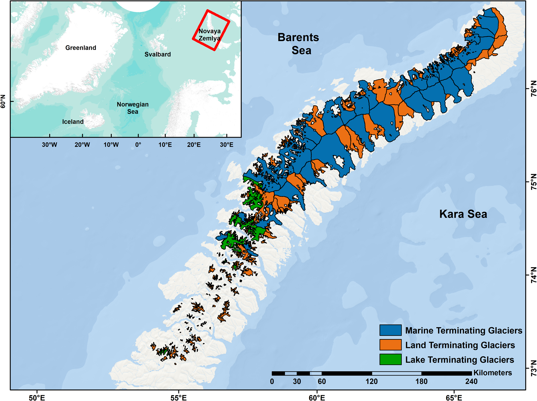
Figure 1. Study area of Novaya Zemlya, with RGI 6.0 glacier outlines shown. The ESRI World Ocean and World Terrain basemaps are used in the background.
Data and methods
Data
Landsat images have proven to be an effective asset for glacier mapping, and for creating multi-temporal outlines of glaciers due to its large swath width, its multispectral capabilities and its long temporal record of capturing images for over five decades (e.g. Nuth and others, Reference Nuth2013). A total of 16 images from Landsat 5 Thematic Mapper (TM), Landsat 7 Enhanced Thematic Mapper Plus (ETM+) and Landsat 8 Operational Land Imager (OLI) are used in this study (Table 1), divided into three time periods: 1986–89, 2000–01 and 2019–21. The images used were carefully selected with minimal cloud cover.
Table 1. Details of the Landsat images that are used in this study
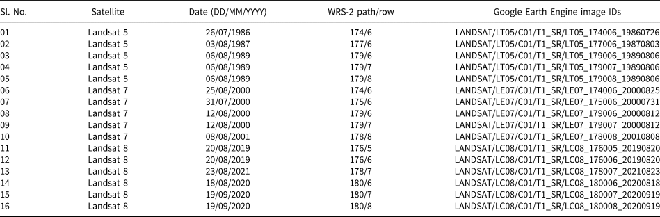
Landsat is a collaborative effort of the USGS and NASA and has been continuously observing the Earth from 1972 until the present day (Wulder and others, Reference Wulder2022). The USGS provides Landsat products in three categories: real-time (RT), tier 1 and tier 2 which are stored in Collection 1 or 2. Tier 1 images have the best quality, and are considered suitable for time-series analysis (Masek and others, Reference Masek2020), while tier 2 images have issues with geometric correction but are still usable. In this study, we use orthorectified level-2 (surface reflectance) images (tier 1) from Collection 1 for mapping glaciers in Novaya Zemlya. Some studies have used raw radiance or digital number (DN) values for glacier mapping with no atmospheric or topographic correction (Paul and others, Reference Paul, Kääb, Maisch, Kellenberger and Haeberli2002; Alifu and others, Reference Alifu, Tateishi and Johnson2015). However, surface reflectance data are essential for systematic analysis, particularly in highly automated approaches (Hemati and others, Reference Hemati, Hasanlou, Mahdianpari and Mohammadimanesh2021).
Method
Google Earth Engine is a cloud-based remote-sensing platform with planetary-scale analysis capabilities that contains a multi-petabyte catalogue of satellite imagery and geospatial datasets, making Google Earth Engine one of the most powerful remote-sensing analysis tools available for analysing change datasets (Gorelick and others, Reference Gorelick2017). Using Google Earth Engine, we developed an object-based image analysis approach for classifying imagery, instead of a simpler pixel-based approach. Pixel-based classification focuses on individual pixels and neglects additional contextual information contained in surrounding pixels that could be used to increase the accuracy such as the spatial relationship with surrounding pixels, size of objects, texture and shape that object-based image analysis incorporates (Blaschke, Reference Blaschke2010).
The method was initially developed using a single Landsat 8 OLI/TIRS image before being applied to the other image sets for the whole of Novaya Zemlya to map glacier changes. This study utilizes six bands from visible to SWIR (OLI bands 2–7), and one thermal infrared band (TIR; TIRS band 10) as input layers for image segmentation (Fig. 2). The visible to SWIR bands have 30 m resolution. The TIR band was originally collected with 100 m resolution, but Google Earth Engine automatically resampled this using a cubic convolution method to 30 m.
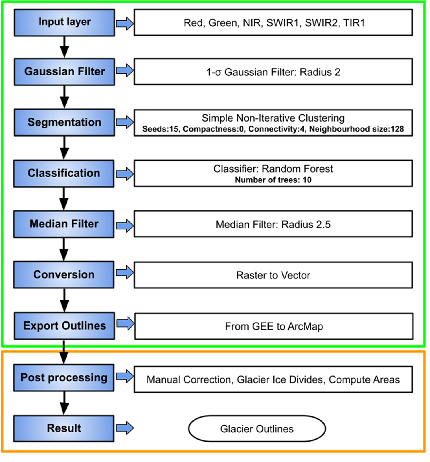
Figure 2. Workflow of the method for creating glacier outlines in Google Earth Engine. The green box shows the automated steps in Google Earth Engine, while the orange box shows the post-processing steps in ArcMap 10.5.1.
In the object-based image analysis approach, segmentation is an important step that groups similar pixels into a cluster or image objects (Ren and Malik, Reference Ren and Malik2003). Pixel-based classification can result in so-called ‘salt and pepper’ noise, and segmentation helps to reduce this effect in the final classification (Ma and others, Reference Ma2019). To reduce noise in the images, a one-sigma Gaussian filter of radius 2 was applied before segmentation (Xue and others, Reference Xue2018).
Google Earth Engine mainly supports three image segmentation techniques for remote sensing: simple non-iterative clustering, k-means and G-means (Liu and others, Reference Liu2018). We use simple non-iterative clustering (Achanta and Süsstrunk, Reference Achanta and Süsstrunk2017), which is an improved version of simple linear clustering, to segment the Landsat image (Fig. 3b). The important parameters of simple non-iterative clustering are compactness, connectivity, seeds or grid size and neighbourhood size. The compactness parameter defines the smoothness of the clusters, which affects cluster shape (Shafizadeh-Moghadam and others, Reference Shafizadeh-Moghadam, Khazaei, Alavipanah and Weng2021). A compactness value of zero removes spatial distance weighting, meaning that clusters are created based only on spectral characteristics. The connectivity parameter deals with adjacent objects, with a connectivity of four corresponding to only orthogonal neighbours, and a connectivity of eight corresponding to orthogonal and diagonal neighbours. The seed/size parameter determines the initial location or spacing of the cluster centres, and neighbourhood size is used to avoid boundary artefacts between tiles (Tassi and Vizzari, Reference Tassi and Vizzari2020). In this study, the parameters compactness = 0, connectivity = 4, seed grid spacing of 15 pixels and neighbourhood size = 128 pixels were selected by repeated iteration and visual evaluation.
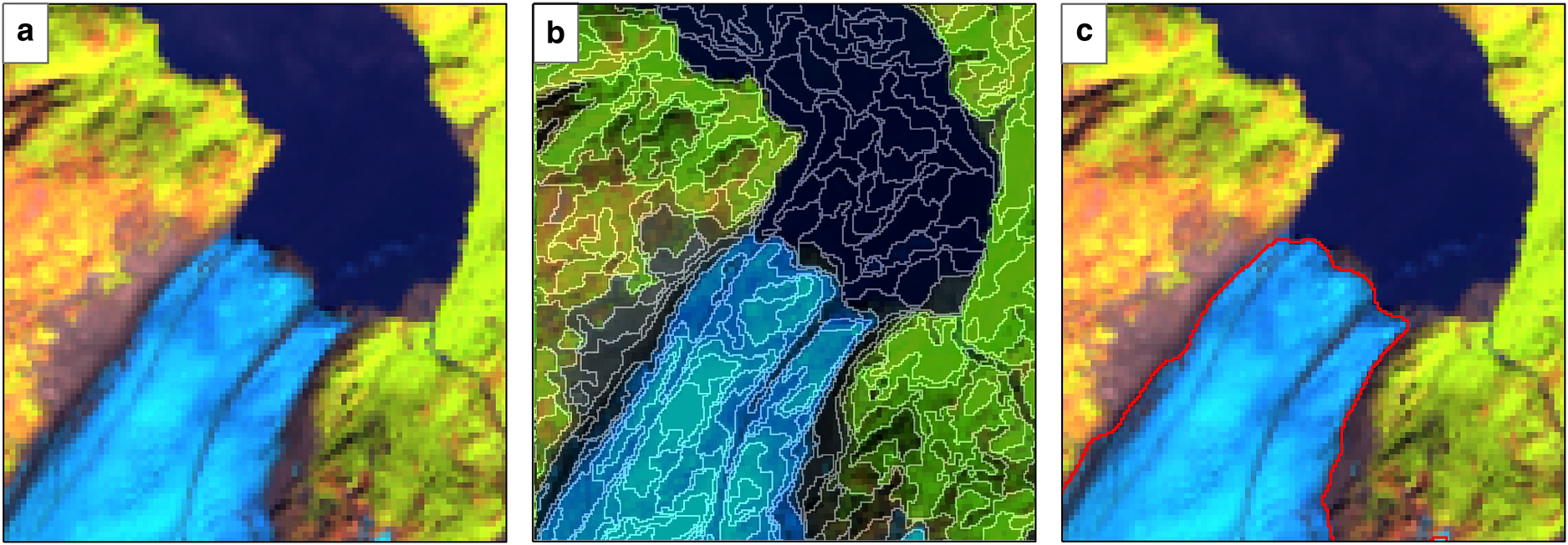
Figure 3. Process of generating outlines using an object-based image analysis approach in Google Earth Engine: (a) a false colour composite of a Landsat 8 image (OLI bands SWIR1, NIR and red); (b) the result of simple non-iterative clustering segmentation and (c) the final glacier outline, overlain on the original image.
The random forest classifier was implemented in Google Earth Engine for the classification of the segmented image. The random forest algorithm is a supervised machine learning algorithm that combines the output of multiple decision trees to produce a single result (Kulkarni and Lowe, Reference Kulkarni and Lowe2016). For image classification, random forest is the most widely used machine learning algorithm in Google Earth Engine (Amani and others, Reference Amani2020). Random forest is robust, easier to implement, capable of dealing with high dimensionality and can reduce the risk of overfitting (Nery and others, Reference Nery2016; Praticó and others, Reference Praticó, Solano, Di Fazio and Modica2021).
In this study, the random forest algorithm using ten trees was trained on manually selected samples of ‘glacier’ and ‘non-glacier’ throughout the scene, and the segments were classified into two main classes: ‘glacier’ and ‘non-glacier’. The ‘glacier’ class includes ice, debris-covered ice and moraines, while the non-glacier class includes water, vegetation, sea-ice, bare land and seasonal snow patches. To train the classifier, we used a total of 728 samples for the 1986–89 images, including 365 glacier samples and 363 non-glacier samples. For the 2000–01 images, we used 317 glacier and 303 non-glacier samples and for the 2019–21 images we used 339 glacier and 367 non-glacier samples.
Finally, a median filter with radius 2.5 was applied to reduce noise in the classified image, and the classified image was converted from raster to vector to create glacier outlines (Fig. 3c). The automated glacier outlines were exported from Google Earth Engine to ArcMap 10.5.1 for post processing. As a final step, each glacier was visually examined to see if manual correction was required, and manual corrections were made where necessary. Finally, the linked glacier outlines were separated using the internal boundaries of the RGI 6.0, to enable examination of the changes in each glacier.
Accuracy and uncertainty
The temporal nature by which satellite images are captured invariably means that images of the same area are captured during different conditions, and there can be seasonal variations that can impact image quality. These variations can be illumination differences, cloud cover or shadows cast over the target feature; for glacier mapping, seasonal snow patches can remain on the ground which are spectrally similar to snow-covered glaciers. Because of this, it is important to understand the capabilities of the method when utilizing images from different times and to assess how accurate the glacier areas are computed using this automated methodology without manual corrections. Therefore, to determine the uncertainty in the glacier area, two approaches were used: random sampling and buffer analysis.
Uncertainty by random sampling
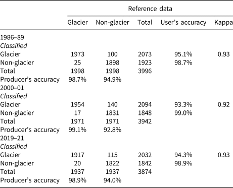
To assess the accuracy of the automated outlines from each period, random samples were generated for each class in ArcMap 10.5.1, using the manually corrected outlines as reference data. The random samples were separated into two classes: ‘glacier’ and ‘non-glacier’, with an equal number of samples for each class. In total, 1998 samples for each class were taken for the 1986–89 outlines; 1971 samples from each class for the 2000–01 outlines and 1937 samples from each class for the 2019–21 outlines. These points were intersected with the automatically generated outlines and the reference data, and confusion matrices were created (Table 2).
Table 2. Confusion matrices of each layer generated based on random sampling
Uncertainty using buffer analysis
To assess the area uncertainty of the manually corrected outlines, a buffer of ±30 m was applied to each manually corrected layer. In the absence of suitable reference data, the buffer approach is typically employed to determine accuracy using a literature-derived uncertainty value (±0.5 or 1 pixel; Granshaw and Fountain, Reference Granshaw and Fountain2006; Paul and others, Reference Paul2017). The uncertainty in the glacier area was determined by calculating the buffered area of each layer. The high, low and area ± uncertainty values for each period are shown in Table 3.
Table 3. Computed areas (in km2) of each layer based on the ±30 m buffer

Results
In 1986–89, the total glacierized region of Novaya Zemlya was 22 990 ± 301 km2, in 2000–01 the area was 22 525 ± 308 km2 and by 2019–21 the glacier area was reduced to 21 670 ± 292 km2. Of the 480 glaciers mapped, 142 are >10 km2, 262 glaciers are between 1 and 10 km2 and 76 glaciers are <1 km2. This glacier inventory includes three terminus types: 38 marine-terminating, 424 land-terminating and 18 lake-terminating glaciers. The marine-terminating glaciers cover the most glacier area (14 448 ± 137 km2), followed by the land-terminating glaciers covering 7299 ± 94 km2 and the lake-terminating glaciers that cover 1241 ± 16 km2.
The overall accuracy for each layer was calculated using the confusion matrices (Table 2). The 1986–89 layer showed 96.8% overall accuracy, the 2000–01 layer had 96.0% accuracy and the 2019–21 layer had 96.5% accuracy. The details of producer's and user's accuracy are mentioned in Table 2. The producer's accuracy varies between 92.8 and 98.9%, the user's accuracy ranges between 93.3 and 99.0% and the kappa coefficient is ⩾0.92 for all three layers.
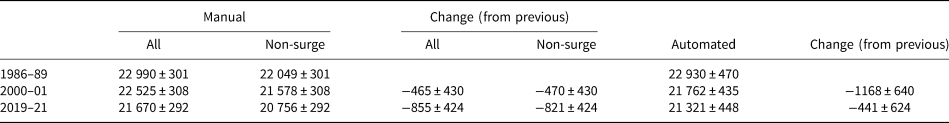
It is also important to assess how accurate the automatically generated glacier areas are, using the information displayed in Table 2. Table 4 compares the manually estimated glacier areas with the unbiased estimates of glacier area for each time period, calculated following the methods described by Olofsson and others (Reference Olofsson, Foody, Stehman and Woodcock2013). The comparison of manual and automated area estimates shows that besides 2000–01, the manual and automated area estimates overlap within the uncertainty bands. When compared to 1986–89 and 2000–01, the manual area estimate shows that the area loss nearly doubled between 2000–01 and 2019–21, whereas the automatic estimate shows the opposite. Additionally, the automated estimate of the area change between 2000–01 and 2019–21 has a larger uncertainty (±624 km2) than the estimated change (−441 km2).
Table 4. Total area (in km2) of glaciers computed from manually corrected outlines (±1 pixel buffer), both including and excluding glaciers that surged, and the automatically generated outlines (±95% confidence interval)
Glacier area changes
To calculate area changes, we use the manually corrected glacier outlines. Between 1986–89 and 2019–21, glaciers in Novaya Zemlya showed a 5.8% reduction in total area. Glacier retreat rates increased by 1.7% from 2000–01 to 2019–21 (−3.8%), compared to from 1986–89 to 2000–01 (−2.1%). These changes in glacier area were not constant across glacier terminus type (land-, lake- and marine-terminating). From 1986–89 to 2019–21, land-terminating glaciers lost 580 ± 130 km2 (7.9%), lake-terminating glaciers lost 106 ± 21 km2 (9.9%), and marine-terminating glaciers lost 605 ± 263 km2 (4.4%) of glacierized area (Fig. 4).
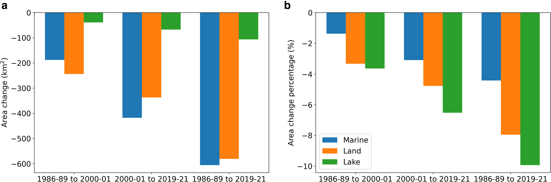
Figure 4. Total area change for lake, marine and land-terminating glaciers in both km2 (a) and per cent area (b).
Figure 5a depicts the area lost for each glacier from 1986–89 to 2000–01 and Figure 5b shows the loss of each glacier from 2000–01 to 2019–21, while Figures 5c,d show the area loss of each glacier as a percentage. Only 41 glaciers larger than 200 km2 are responsible for nearly half (49.5%) of the area loss in the region, and 272 glaciers are responsible for 84% of the total glacier area loss. Because of the larger area of these glaciers, however, the total percentage loss for these 272 glaciers is <25%.
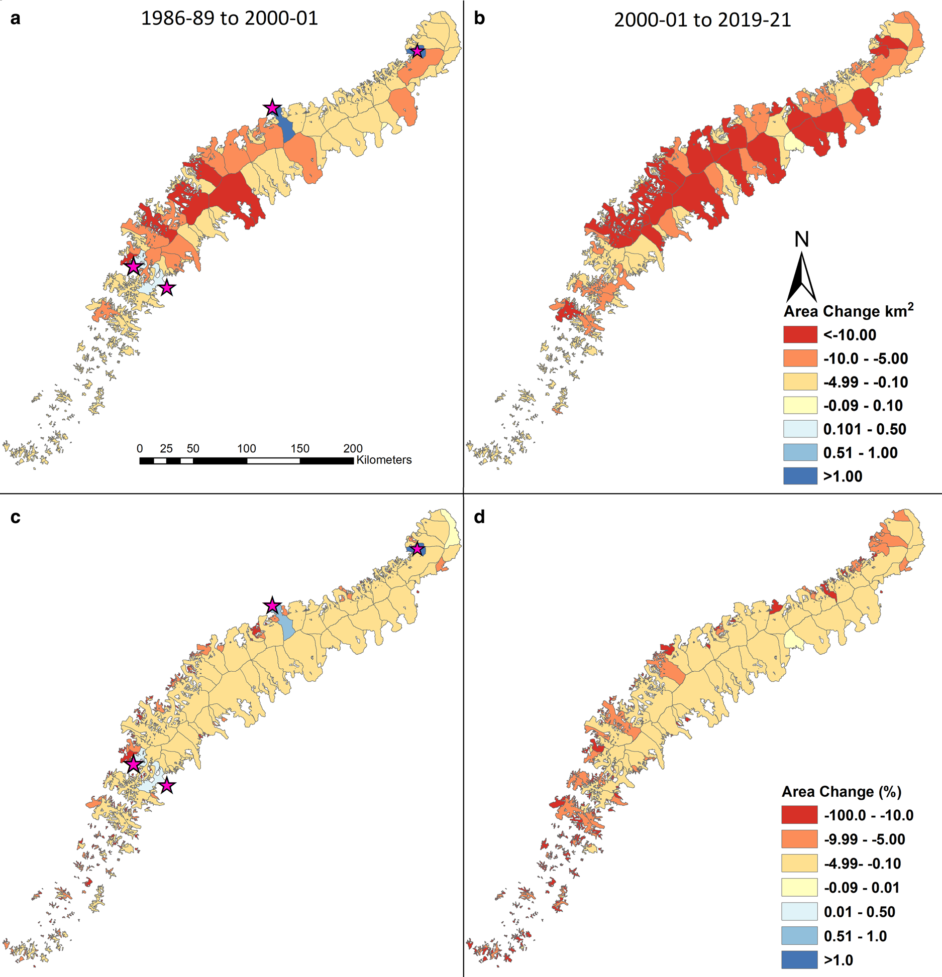
Figure 5. Area changes of Novaya Zemlya glaciers: (a) from 1986–89 to 2000–01 and (b) 2000–01 to 2019–21 in km2, and (c) from 1986–89 to 2000–01 and (d) 2000–01 to 2019–21 as a per cent. Stars in (a) and (c) show glaciers that surged during the 1986–89 and 2000–01 period.
Figure 6 shows the per cent area change vs glacier area based on terminus type. Figure 6b depicts 38 marine-terminating glaciers that cover the majority of the glacierized region (14 448 ± 137 km2) in Novaya Zemlya, Figure 6a shows 18 lake-terminating glaciers which cover 1241 ± 16 km2, while Figure 6c shows 424 land-terminating glaciers covering 7299 ± 94 km2. In between 1986–89 and 2019–21, three land-terminating glaciers have completely disappeared, and 18 glaciers retreated more than 60%, while a further 57 glaciers retreated between 40 and 60%.
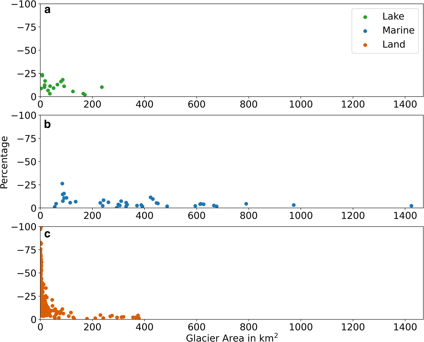
Figure 6. Per cent area change vs glacier area for each glacier from 1986–89 to 2019–21, for (a) lake-terminating, (b) marine-terminating and (c) land-terminating glaciers.
Discussion
Glacier retreat
As reported elsewhere (e.g. Sharp and others, Reference Sharp, Kargel, Leonard, Bishop, Kääb and Raup2014; Kochtitzky and Copland, Reference Kochtitzky and Copland2022), it is clear that glaciers are retreating across the Arctic. This study shows that all glaciers in Novaya Zemlya have retreated at various rates from 0.3 to 100%, with a few examples of surging glaciers captured in the analysis (Figs 5a, c). Although the area loss of glaciers differed by each glacier type in Novaya Zemlya. Carr and others (Reference Carr, Bell, Killick and Holt2017) found that the retreat rate of marine-terminating glaciers is higher than that of land-terminating glaciers, which is corroborated by our results (Fig. 4). However, land-terminating glaciers did not experience the same increase in retreat rate as lake- and marine-terminating glaciers in 2000–01 to 2019–21. The retreat rate of land-terminating glaciers increased by 1.4% between 2000–01 and 2019–21 relative to that between 1986–89 and 2000–01, whereas the retreat rates of lake- and marine-terminating glaciers increased by 2.8 and 1.7%, respectively.
Like the rest of the Arctic, Novaya Zemlya is warming faster than the rest of the world, with both surface air and sea surface temperatures increasing rapidly over both the Barents and Kara Sea coasts (e.g. Kohnemann and others, Reference Kohnemann, Heinemann, Bromwich and Gutjahr2017; Isaksen and others, Reference Isaksen2022). In particular, Isaksen and others (Reference Isaksen2022) found that 2 m surface air temperature warming was higher on the Barents Sea side of Novaya Zemlya (1.5–2.0$^\circ$ C decade−1 between 1981–2020) compared to the Kara Sea side (1.0–1.5$^\circ$
 C decade−1). These changes are driven in part by a decrease in sea ice concentration (SIC) in the region (Yamagami and others, Reference Yamagami, Watanabe, Mori and Ono2022), with the drop in SIC over the Barents Sea nearly twice as high compared to the Kara Sea (Kumar and others, Reference Kumar, Yadav and Mohan2021a). Consistent with these studies, our observations show that glaciers terminating on the Barents Sea coast of Novaya Zemlya retreated faster than glaciers terminating on the Kara Sea coast (Fig. 7), a pattern that remains consistent across glacier terminus type (Fig. 8). Barents Sea glaciers lost a total area of 843.4 km2 (−7.3%) between 1986–89 and 2019–21, while glaciers on the Kara Sea lost 448.9 km2 (−4.2%).
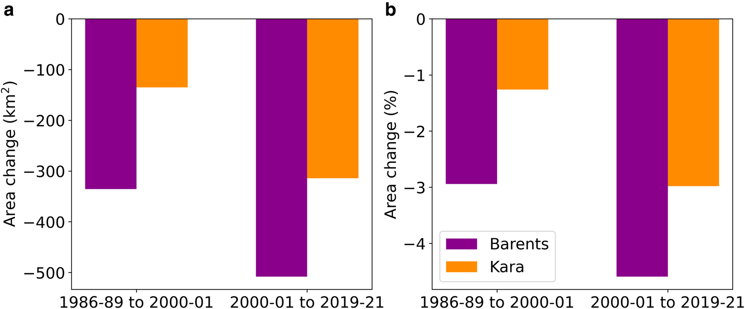
Figure 7. Area change for glaciers on the Barents Sea vs Kara Sea (a) in km2 and (b) as a percentage.
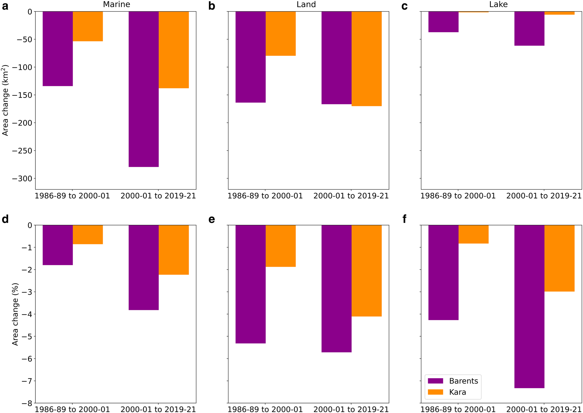
Figure 8. Area change of marine (a, d), land (b, e) and lake-terminating (c, f) glaciers on the Barents Sea vs Kara Sea, in km2 (a–c) and per cent area (d–f).
Examination based on terminus type shows that all three types of glaciers are retreating more on the Barents Sea side than those terminating on Kara Sea side (Fig. 8). Carr and others (Reference Carr, Stokes and Vieli2014) observed a similar pattern of higher retreat on the Barents Sea coast than the Kara Sea between 1992 and 2010. Marine- and lake-terminating glaciers are retreating faster on both sides, in both time periods of the study, although land-terminating glacier retreat is slowing down at the Barents Sea in 2000–01 to 2019–21 compared to 1986–89 and 2000–01.
All three types of glaciers: lake-, marine-, and land-terminating have lost more glacier area from 2000–01 to 2019–21 than 1986–89 to 2000–01; although, during the period 1986–89 to 2000–01, three marine-terminating glaciers and one lake-terminating glacier surged. Two of the same glaciers were identified by Carr and others (Reference Carr, Bell, Killick and Holt2017), and one was identified by Grant and others (Reference Grant, Stokes and Evans2009). This study identified one additional glacier surge (Pavlov Glacier, RGI 6.0 ID: RGI60-09.00070) that increased the area of the glacier by 3.2 km2, and showed terminus advance by up to 1.3 km by 2000–01 compared to 1986–89 (Fig. 9). No glacier surges were observed in the land-terminating glaciers. During 1986–89 to 2000–01, all four surged glaciers increased in area by 0.6% (+5.8 km2), however during the second time period (2000–01 to 2019–21), the same glaciers retreated and showed a strongly negative change in area of −3.4% (−32.6 km2), with a net area loss between 1986–89 and 2019–21 for each glacier. These four glacier were excluded from the area change analysis.
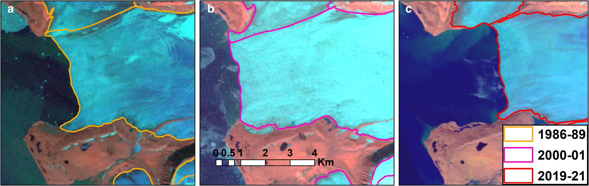
Figure 9. Time series of Landsat images showing Pavlov Glacier (RGI60-09.00070) in (a) 1986-07-26, (b) 2000-07-31 and (c) 2019-08-20, showing a clear advance associated with a surge between 1986 and 2000.
Comparison of glacier area loss with mass-balance loss
Comparing glacier area changes with geodetic mass balances obtained from Hugonnet and others (Reference Hugonnet2021) for the period 2000–20 shows that marine-terminating glaciers lost both area (3.1%) as well as mass (−0.25 m a−1) and lake-terminating glaciers lost a total of 6.5% area while also showing greater mass loss (−0.42 m a−1) compared to land- and marine-terminating glaciers (Fig. 10). However, land-terminating glaciers show a slightly different pattern than lake- and marine-terminating glaciers (Fig. 10), with land-terminating glaciers losing a substantial amount of area (4.7%) with less substantial mass loss (−0.18 m a−1).
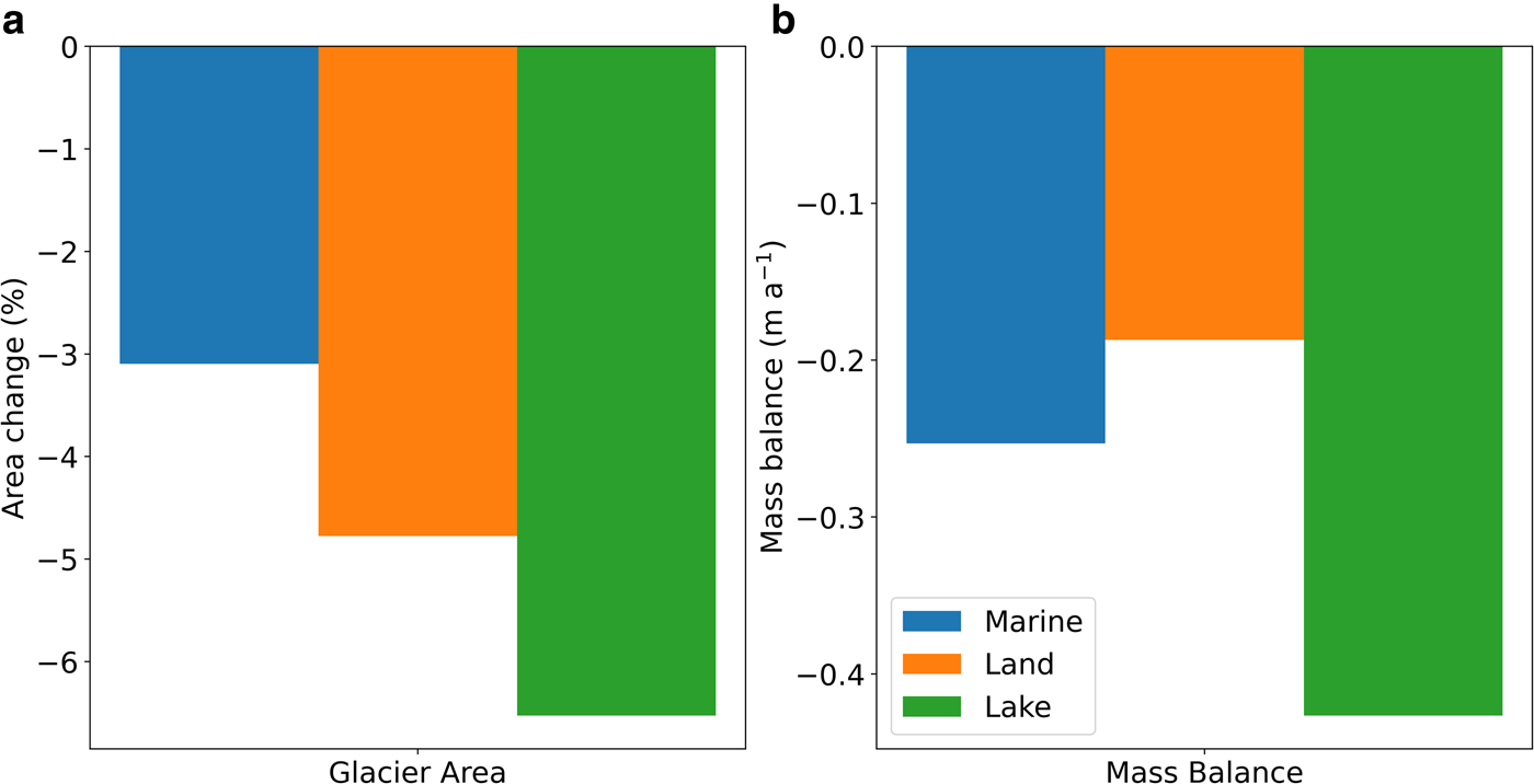
Figure 10. (a) Per cent area change (2000–01 to 2019–21) and (b) area-averaged mass change (2000–20) from Hugonnet and others (Reference Hugonnet2021) for each glacier type.
Figure 11 depicts a comparison of each glacier area loss with its mass loss. The results indicate that lake-terminating glaciers lost more area than land and marine-terminating glaciers (Fig. 10), with a more negative mass balance (Fig. 11). Ciracì and others (Reference Ciracì, Velicogna and Sutterley2018) found that marine-terminating glaciers are losing mass faster than glaciers terminating on land. Almost the same trend can be seen in marine-terminating glaciers, with a more negative area-averaged mass balance for marine-terminating glaciers compared to land-terminating glaciers (Fig. 11), because marine- and lake-terminating glaciers lose mass via frontal ablation and land-terminating glaciers do not. Land-terminating glaciers showed the least mass loss compared to marine- and lake-terminating glaciers, as seen in the total mass loss of land-terminating glaciers (Fig. 10). In terms of relative area change, however, land-terminating glaciers showed a stronger decrease in area compared to marine-terminating glaciers.
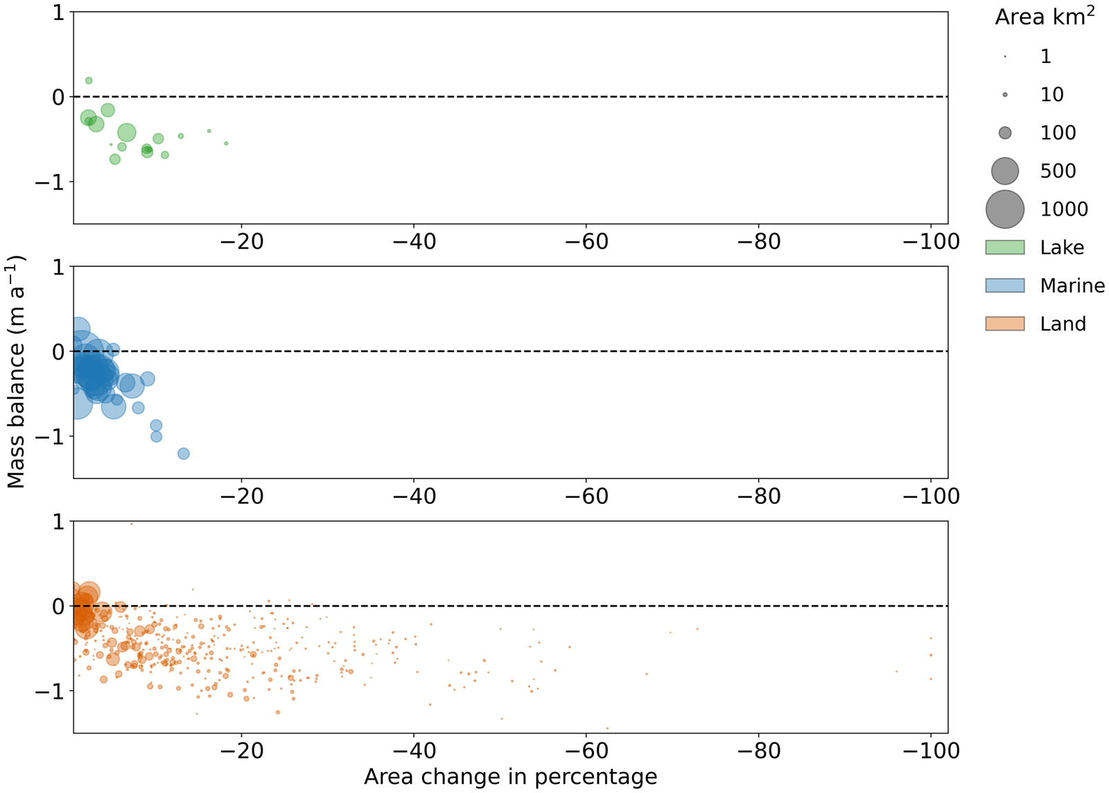
Figure 11. Area-averaged mass change (2000–20) from Hugonnet and others (Reference Hugonnet2021) vs per cent area change (2000–01 to 2019–21) for each glacier.
Methodology framework in Google Earth Engine
Rastner and others (Reference Rastner, Bolch, Notarnicola and Paul2013) compared object-based image analysis with pixel-based classification using the red/SWIR band ratio technique, demonstrating that object-based image analysis performed better than pixel-based classification and reduced the time needed for manual corrections, despite the longer processing time required.
The 16 level-2 products used in this study total 9.10 GB as distributed by USGS Earth Explorer. Downloading the files via the USGS Bulk Download Web Application took ~15 min, even on a fast internet connection. In comparison, running the script to generate outlines for a single image on Google Earth Engine and exporting the outlines took ~1 min.
In addition to the time saved by forgoing downloading and processing the images locally, the object-based image analysis method implemented on Google Earth Engine reduced the amount of manual correction needed when compared to the red/SWIR1 band ratio method. Figure 12 compares the object-based image analysis output to the manually corrected outlines, as well as the output of the red/SWIR1 band ratio using a threshold of 2.0, following Rastner and others (Reference Rastner, Strozzi and Paul2017). Both outputs clearly require manual correction, with large areas of seasonal snow captured by both methods in the area shown in Figure 12a, but the band ratio output captures a large area of seasonal and perennial snow patches (Fig. 12b) that is not captured by the object-based image analysis output. In addition, both methods have misclassified areas of thin cloud cover, shown in the middle of Figure 12b, as well as areas with larger medial moraines.
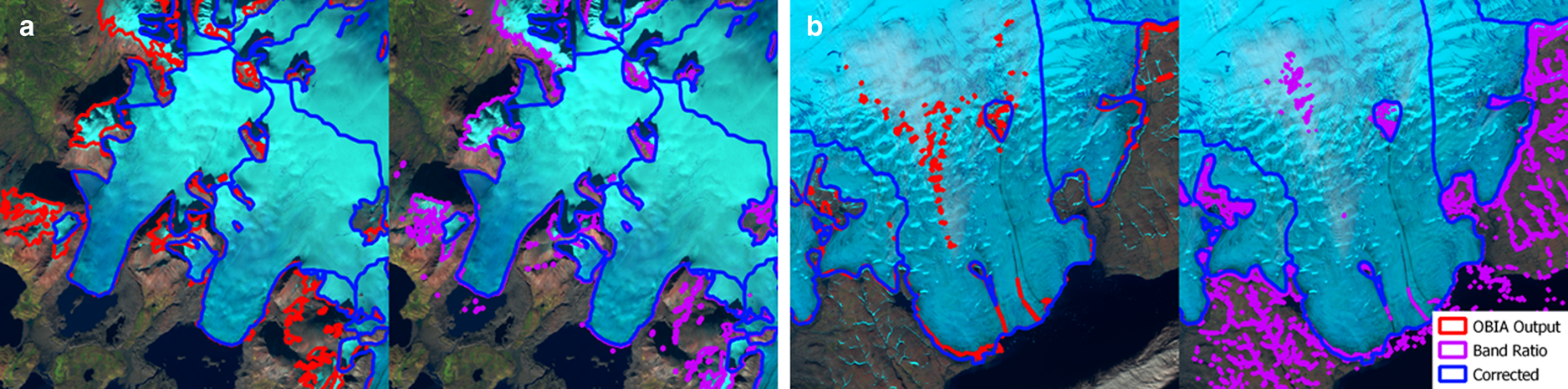
Figure 12. Comparison between object-based image analysis, band ratio and corrected outlines for two different sites in Novaya Zemlya.
In this study, the Google Earth Engine object-based image analysis approach removes the time required for downloading, extracting and storing the images, is easily applicable to other regions, and reduces the amount of manual correction required, as compared to pixel-based methods. This method, however, may not be effective for mapping debris-covered glaciers, or areas covered by fresh snow or thin cloud cover. To address these issues, other approaches that have used object-based image analysis have included additional datasets such as DEMs and terrain slope or coherence derived from synthetic aperture radar images (Robson and others, Reference Robson2015, Reference Robson, Hölbling, Nuth, Strozzi and Dahl2016). Unfortunately, many of these products are not yet available in Google Earth Engine, though the possibility exists for users to upload and make use of these additional datasets in their workflows.
Conclusion
This study presents a new object-based image analysis methodology, implemented in Google Earth Engine, for rapid and accurate glacier mapping. The software framework designed in Google Earth Engine utilizes multi-temporal Landsat satellite imagery, and the outlines generated showed an accuracy of between 96 and 97% when compared to a manually corrected reference dataset. This demonstrates that our methodology is a powerful, robust tool for accurate and rapid mapping of glaciers changes on regional scale that reducing the time required of manual correction and can be applied to other glacierized regions. Utilizing this automated approach, we created outlines of glaciers on Novaya Zemlya for three different time periods: 1986–89, 2000–01 and 2019–21. This important dataset is essential for understanding the impact of climate change on glaciers, and could be used to estimate ice volume and mass change.
This method allowed for a comprehensive analysis of the changes that occurred in Novaya Zemlya glaciers between 1986–89 and 2019–21. Over this time period, glaciers in Novaya Zemlya lost a total area of 1292 ± 419 km2 (5.8%), with three glaciers disappearing entirely. The results clearly demonstrate that all glaciers in Novaya Zemlya are responding to the impacts of climatic warming in the Arctic. With the exception of four glaciers that surged between 1986–89 and 2000–01, all glaciers in the study area retreated between 1986–89 and 2019–21, and even those four glaciers have retreated since 2000–01.
Our analysis indicates there are regional variations in how glaciers are responding to oceanic warming in this part of the Arctic, with more loss observed from glaciers that terminate on the Barents Sea side of Novaya Zemlya compared to those that terminate on the Kara Sea side. In comparison, results showed that land-terminating glaciers retreated less between 2000–01 and 2019–21 compared to 1986–89 and 2000–01, while the retreat rate of marine-terminating glaciers increased from 2000–01 to 2019–21, relative to 1986–89 to 2000–01. While marine-terminating glaciers, which cover the majority of Novaya Zemlya, lost more area than land- and lake-terminating glaciers, lake-terminating glaciers showed a larger percentage loss than the land- and marine-terminating glaciers.
Detailed regional studies of glacier behaviour across the Arctic are important for understanding the decadal responses and the likely trajectory of Arctic glaciers in a warming world. Given their potential contribution to global sea levels it is important to map and understand the scale of change accurately and to provide tools for rapid assessment at regional scales. Platforms such as Google Earth Engine, combined with the expansive Landsat archive and approaches such as object-based image analysis, help provide these tools.
Data
The manually corrected glacier outlines are available from the Global Land Ice Measurements from Space (GLIMS) database at http://www.glims.org/. An example Google Earth Engine script demonstrating the object-based image analysis process can be accessed at the following link: https://code.earthengine.google.com/?accept_repo=users/buner_shapfile/OBIA_Example_code.
Acknowledgements
This work was carried out as part of Asim Ali's PhD project, funded by an Ulster University Vice Chancellor's Research Studentship. Landsat images used in Google Earth Engine were provided by courtesy of the US Geological Survey. We thank James Lea, two anonymous reviewers and the editors for their constructive and insightful comments, which helped improve the quality of the manuscript.
Author contributions
AA developed the method, performed data analysis and interpretation, created figures and wrote the initial draft of the manuscript. PD, SC, DK and RM helped with conceptualization, methods, analysis and editing. RM also assisted with developing the method, creating figures and interpretation. RN helped with writing and editing the manuscript. All authors reviewed results and approved the final version of the manuscript.


 Open access