


INTRODUCTION
The Hindu Kush–Karakoram–Himalayan (HKH) region is the storehouse of fresh water of South Asia (Raina and Srivastava, Reference Raina and Srivastava2008; Bajracharya and others, Reference Bajracharya2015). The glaciers of the Himalaya contribute significantly to the overall river runoff of south and southeast Asia (Basnett and others, Reference Basnett, Kulkarni and Bolch2013) with the highest contribution from the Indus River which originates in the northwest Himalaya (Immerzeel and others, Reference Immerzeel, van Beek and Bierkens2010; Basnett and others, Reference Basnett, Kulkarni and Bolch2013). Himalayan glaciers have been in a general state of recession since 1850 (Mayewski and Jeschke, Reference Mayewski and Jeschke1979; Bhambri and Bolch, Reference Bhambri and Bolch2009; Shukla and others, Reference Shukla, Ali, Hasan and Romshoo2017), except for emerging indications of stability or mass gain in the Karakoram (Hewitt, Reference Hewitt2005; Reference Hewitt2011; Bolch and others, Reference Bolch2012; Bhambri and others, Reference Bhambri, Hewitt, Kawishwar and Pratap2017). Recent comprehensive study by Bhambri and others (Reference Bhambri, Hewitt, Kawishwar and Pratap2017) reported that the number of surge-type glaciers in the Karakoram have increased significantly. This asymmetrical behavior of the Karakoram glaciers could be attributed to regional topography (Scherler and others, Reference Scherler, Bookhagen and Strecker2011a, Reference Scherler, Bookhagen and Streckerb), regional climate (Bashir and others, Reference Bashir, Zeng, Gupta and Hazenberg2017), glacier hypsometry (Gardelle and others, Reference Gardelle, Berthier and Arnaud2012; Brun and others, Reference Brun, Berthier, Wagnon, Kääb and Treichler2017), the characteristics and thickness of supraglacial debris cover (Scherler and others, Reference Scherler, Bookhagen and Strecker2011a) and their morphological properties (Salerno and others, Reference Salerno2017).
In the HKH region, a paucity of appropriate glacier data has prevented a comprehensive assessment of current regional mass balance (Bolch and others, Reference Bolch2012; Kääb and others, Reference Kääb, Berthier, Nuth, Gardelle and Arnaud2012). Multi-temporal and multi-spectral remotely sensed images are being used to detect changes in glacier area (Bhambri and others, Reference Bhambri, Bolch, Chaujar and Kulshreshtha2011), length or terminus position (Bhambri and others, Reference Bhambri, Bolch and Chaujar2012), velocity (Kraaijenbrink and others, Reference Kraaijenbrink2016) and thickness (Bolch and others, Reference Bolch, Buchroithner, Pieczonka and Kunert2008) with large spatial scale at regular temporal intervals. Several interlinked global glaciers inventory initiatives exist, such as World Glacier Monitoring Service (WGMS; Haeberli and others, Reference Haeberli, Bosch, Scherler, Ostrem and Wallen1989), Global Land Ice Measurements from Space (GLIMS; Raup and others, Reference Raup2007), GlobGlacier project (Paul and others, Reference Paul2009), Randolph Glacier Inventory (RGI; Pfeffer and others, Reference Pfeffer2014), Glacier Area Mapping for Discharge in Asian Mountains (GAMDAM; Nuimura and others, Reference Nuimura2015) and International Centre for Integrated Mountain Development (ICIMOD; Bajracharya and Shrestha, Reference Bajracharya and Shrestha2011; Bajracharya and others, Reference Bajracharya2015). However, none of the initiatives has resulted in an accurate and complete glacier inventory for the Himalayan region. Of all others, field investigation and measurement becomes an indispensable element of glaciology to overcome the uncertainties and speculations derived from the remotely sensed satellite datasets (Hubbard and Glasser, Reference Hubbard and Glasser2005).
Studies on glaciers located in the Western Himalaya (e.g. Beas, Chenab and Sutlej) have been done either using the Survey of India (SoI) topographical maps or coarser spatial resolution satellite datasets (Kulkarni and Alex, Reference Kulkarni and Alex2003; Kulkarni and others, Reference Kulkarni2007; Sharma and others, Reference Sharma2016; Brahmbhatt and others, Reference Brahmbhatt2017). However, several published works have registered inaccuracies in the portrayal of glacier outline on the SoI topographical maps of the 1960s (Bhambri and others, Reference Bhambri, Bolch, Chaujar and Kulshreshtha2011; Chand and Sharma, Reference Chand and Sharma2015). It is further observed that on the coarser resolution satellite datasets (e.g. Landsat Multispectral Scanner), it is difficult to identify glacier terminus precisely, especially in the case of debris-covered glaciers (Chand and Sharma, Reference Chand and Sharma2015). The declassified imagery of Corona and Hexagon acquired in the 1960s and the 1970s provide great possibility to extract the historic glacier outlines for comparison with contemporary glacier outlines derived from satellite images (Schmidt and Nüsser, Reference Schmidt and Nüsser2009, Reference Schmidt and Nüsser2012, Reference Schmidt and Nüsser2017; Bhambri and others, Reference Bhambri, Bolch, Chaujar and Kulshreshtha2011; Chand and Sharma, Reference Chand and Sharma2015; Bhattacharya and others, Reference Bhattacharya2016). Only a few studies exist on mapping and monitoring of glaciers for Chandrabhaga basin (Kulkarni and others, Reference Kulkarni, Dhar, Rathore, Govindha and Kalia2006; Negi and others, Reference Negi, Saravana, Rout and Snehmani2013; Pandey and Venkataraman, Reference Pandey and Venkataraman2013; Birajdar and others, Reference Birajdar, Venkataraman, Bahuguna and Samant2014; Garg and others, Reference Garg, Shukla, Tiwari and Jasrotia2017a) while several studies have been published on mapping and change analysis of glaciers of the adjacent basins (Kamp and others, Reference Kamp, Byrne and Bolch2011; Schmidt and Nüsser, Reference Schmidt and Nüsser2012, Reference Schmidt and Nüsser2017; Chand and Sharma, Reference Chand and Sharma2015; Murtaza and Romshoo, Reference Murtaza and Romshoo2016; Brahmbhatt and others, Reference Brahmbhatt2017; Chudley and others, Reference Chudley, Miles and Willis2017; Rashid and others, Reference Rashid, Romshoo and Abdullah2017; Patel and others, Reference Patel, Sharma, Fathima and Thamban2018). However, to the best of our knowledge, there is no published study on the Jankar Chhu Watershed (JCW) addressing glacier change in association with other variables (e.g. debris cover, topography and climate parameters). In addition, no studies exist that use declassified Corona images for glacier change analysis in the JCW. Thus the main goals of this study are to (i) generate a complete and up-to-date glacier inventory for the JCW, Chandrabhaga basin using Sentinel 2A (2016) images aided by high-resolution Google Earth (GE) images and limited field observation; (ii) analyze glacier area change in the JCW for 1971 (Corona), 2000 (Landsat) and 2016 (Sentinel 2A); and (iii) evaluate the possible impact of climate variables on glacier changes in the JCW.
STUDY AREA
The JCW is located in Lahaul and Spiti district of Himachal Pradesh, northern India. The total area of the JCW is 694.5 km2, where altitude varies from 3305 to 6309 m a.s.l. in the upper Chenab River system of the Greater Himalaya range (Fig. 1a). In the local language, ‘Chhu’ is the synonym of the small river. The Jankar Chhu is a tributary of Bhaga River and confluences at Darcha (32°40′N and 77°12′E; ~3313 m a.s.l.) (Fig. 1b). Chandra and Bhaga River flow together form Chandrabhaga (Chenab), which ultimately contributes to the Indus River system.

Fig. 1. (a) Location of study area in the Western Himalaya and in the upper Chenab River system of the Indian subcontinent. (b) Glacier coverage in the Jankar Chhu Watershed based on Sentinel 2A (1 November 2016) imagery; red and green stars represent field visited and mapped glaciers from Landsat TM (9 October 1989), respectively.
The climate of the study area is dominated by a long winter season from mid-November to March, with a spring season that lasts until the end of May (Owen and others, Reference Owen1996). The region falls under the monsoon-arid transition zone. The region of Lahaul Himalaya is influenced by South Asian monsoon in the summer season and mid-latitudes westerlies in winter (Shehmani and others, Reference Shehmani, Dharpure, Kochhar, Ram and Ganju2015). The JCW has no climate observatory. Patsio (32°45′N; 77°15′E; ~3774 m a.s.l.; 1983–present) in the Bhaga valley is the nearest representative observatory located at the southeast edge of the JCW (Fig. 1b), maintained and operated by the Snow Avalanche Study Establishment (SASE), Government of India. Sharma and others (Reference Sharma2016) have reported that ~80% of annual precipitation in Patsio is contributed through mid-latitude westerlies.
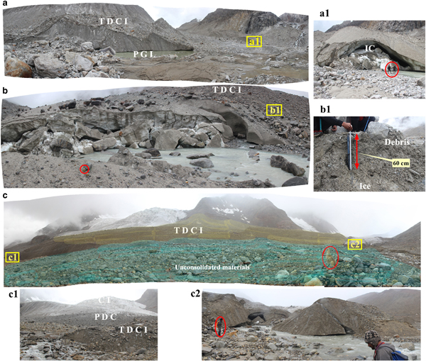
Field observations during 2015–17 of select glaciers show that large valley glaciers in the JCW are characterized by extensive supraglacial debris cover, crevasses, ice caves, lakes and glacial streams (Fig. 2). The terminus position has been measured at one point in the center of the terminus for five glaciers (see Fig. 1b for location) using a handheld GPS (Garmin etrex10 with ±5–10 m horizontal accuracy). Field measurement reveals that debris thickness on glaciers varies from 5 to 60 cm (Fig. 2b).

Fig. 2. Field photographs (2015–17) showing the terminus characteristics of select glaciers in the Jankar Chhu Watershed (see Fig. 1b for location). TDCI, thick debris-covered ice; PDC, partially debris-covered; CI, clean ice; IC, ice collapse; PGL, pro-glacial lake. The red circle and line represent the scale of the image.
DATA SOURCES
Glacier mapping, inventory and change analysis were carried out for the JCW, Chandrabhaga basin, Lahaul Himalaya from various temporal, multi-spectral and medium to high-resolution satellite image sources (Table 1). The Corona (KH-4B) images of 1971, with minimal seasonal snow cover as well as cloud cover acquired from the United States Geological Survey (USGS; http://earthexplorer.usgs.gov/), were used to extract the extent of baseline glacier boundaries in the JCW. Multi-spectral orthorectified Sentinel 2A (2016), Landsat Thematic Mapper (TM; 1989) and Enhanced Thematic Mapper Plus (ETM+; 2000) satellite images were acquired from USGS in the Universal Transverse Mercator (UTM) Zone 43 World Geodetic System (WGS) 84 projection (Table 1). Sentinel 2A and Landsat images were specifically obtained under (or nearly) cloud-free conditions at the end of ablation season. The Advanced Spaceborne Thermal Emission Reflection Radiometer Global Digital Elevation Model Version 2 (ASTER GDEM v2) was used as reference DEM for semi-automatic delineation of drainage basins and extraction of topographic parameters of the glacier (Table 1).
Table 1. Satellite data and Digital Elevation Model (DEM) used in this study
#Radio-metrically corrected and orthorectified images; **radio-metrically corrected; *data downloaded from http://earthexplorer.usgs.gov; +ASTER GDEM (Advanced Spaceborne Thermal Emission and Reflection Radiometer Global Digital Elevation Model) is a product of the Ministry of Economy, Trade, and Industry of Japan (METI) and the National Aeronautics and Space Administration (NASA). GCPs, ground control points; RMSE, root-mean-square error; Pan, panchromatic; KH-4B: keyhole-4B; TM: Thematic Mapper; ETM: Enhanced Thematic Mapper; MSI: multispectral instrument; VIS: visible; IR: infrared; TR: thermal; MIR, mid-infrared; SWIR, shortwave infrared.
METHODS
Rectification of satellite images
Owing to the difficult geometry of the Corona imagery (Schmidt and Nüsser, Reference Schmidt and Nüsser2012; Bhambri and others, Reference Bhambri, Bolch, Chaujar and Kulshreshtha2011, Reference Bhambri, Bolch and Chaujar2012), three subsets of three Corona forward strips were generated in the present study. All subsets were co-registered based on two operational approaches suggested by Bolch and others (Reference Bolch2010b): (1) projective transformation was performed based on ground control points (GCPs) and the ASTER GDEM using ERDAS Imagine 14; followed by (2) spline adjustment using ESRI ArcGIS 10.2.2. Prominent peaks and junctions between streams and roads were used for GCPs assuming no changes occurred for these points on the ground during the observation period. For each Corona subset, 40–320 GCPs were acquired from Sentinel 2A imagery (2016) for co-registration. We concentrated on the adjustment of the area around the glaciers in Corona images with respect to the base image (2016) for consistency of results during rectification (Bolch and others, Reference Bolch2010b; Bhambri and others, Reference Bhambri, Bolch, Chaujar and Kulshreshtha2011). In addition, to assess positional accuracy, 30 common points (e.g. confluence of ridges and road junctions) were carefully identified in each Corona subset and Sentinel 2A image. The horizontal shift of three Corona images was calculated at ±5.6, ±5.4 and ±6.2 m to base image (Sentinel 2A) (Table 1).
The Landsat ETM+ image of 2000 is available in the processing level L1T (radio-metrically calibrated and orthorectified using GCPs and DEM) and Landsat TM image of 1989 processed to L1G (radio-metrically calibrated and non-orthorectified) (Tucker and others, Reference Tucker, Grant and Dykstra2004). Both Landsat images show a horizontal shift of ~30 m as compared with 2016 base image (Sentinel 2A). In addition, Landsat ETM+ comes with a panchromatic band (band 8; ~0.5–0.9 µm) with spatial resolution of 15 m. Bands 1–5 and band 6 of the Landsat ETM+ (2000) were pan-sharpened to 15 m using Brovey transformation image fusion technique with panchromatic band (Chand and Sharma, Reference Chand and Sharma2015). This helps in identifying terminus position and other morphological features (e.g. debris-covered ice, supraglacial ponds, etc.). Landsat TM (1989) and pan-sharpened ETM+ (2000) imagery were coregistered to the base image (Sentinel 2A) using projective transformation as discussed earlier. Thirty common points were identified in Landsat TM (1989), pan-sharpened ETM+ (2000) and base image (Sentinel 2A) to assess the positional accuracy. The horizontal shift between the base image and Landsat pan-sharpened ETM+ and TM was measured at ~10.5 m (~0.7 pixels) and ~11.6 m (~0.4 pixels), respectively. Sentinel 2A image was processed in two steps. At first, visible and near-infrared bands were stacked using layer stacking tool in ERDAS Imagine 14. Later, shortwave infrared band 2 (SWIR2; band 12; 20 m spatial resolution) was resized to 10 m with the stacked band in ERDAS Imagine 14.
Glacier mapping and inventory
Glacier outlines were manually delineated from 1971 Corona images (Fig. 3a). For Landsat TM (1989) and pan-sharpened ETM+ imagery (2000), glaciers were manually mapped using mid-infrared–red–green bands (Fig. 3b). Bands SWIR2–red–green were used for glacier boundary delineation from 2016 Sentinel 2A image (Fig. 3c). The minimum size of mapped glaciers included in our inventory is 0.02 km2 as per Bajracharya and Shrestha (Reference Bajracharya and Shrestha2011) and Frey and others (Reference Frey, Paul and Strozzi2012). Manual on-screen mapping was done despite having advantages of automated band ratio techniques (Paul and others, Reference Paul2009, Reference Paul2013) as the relative error strongly increases with decreasing glacier area (Paul and others, Reference Paul2013; Fischer and others, Reference Fischer, Huss, Barboux and Hoelzle2014) and with the presence of debris cover (Bolch and others, Reference Bolch, Buchroithner, Pieczonka and Kunert2008; Racoviteanu and others, Reference Racoviteanu, Williams and Barry2008; Frey and others, Reference Frey, Paul and Strozzi2012). Paul and others (Reference Paul2013) have shown that the bias significantly increases for glaciers with an area <1 km2 in size, which constitutes ~77.3% of all glaciers in the JCW in 2016, reducing the advantage of automatic techniques. It is important to differentiate between snow packs and small glaciers (<0.5 km2 in size) as some snow packs can sustain for several years. Multi-temporal historical images (e.g. Corona, Landsat) were used to differentiate between these. Several signs of movement (based on overlays of multi-temporal images) such as issuing meltwater streams at the end of the terminus, breaks in surface slope, spectral color differences and the presence of small meltwater ponds were employed for identification of the most likely position of the glacier termini in the study (Bhambri and others, Reference Bhambri, Bolch, Chaujar and Kulshreshtha2011; Chand and Sharma, Reference Chand and Sharma2015). To assist manual delineation of debris-covered terminus in 2016, imagery from GE was used as an additional source in combination with the Sentinel 2A image. Field mapping and photographs also facilitated the determination of glacier termini during 2015–17. Ice and snow areas directly above bergschrunds were not included in the glacier outlines (cf. Racoviteanu and others, Reference Racoviteanu, Paul, Raup, Khalsa and Armostrong2009; Bhambri and others, Reference Bhambri, Bolch, Chaujar and Kulshreshtha2011). In addition, digitized glacier boundaries from Sentinel 2A image were exported to GE for cross-checking and manual correction.
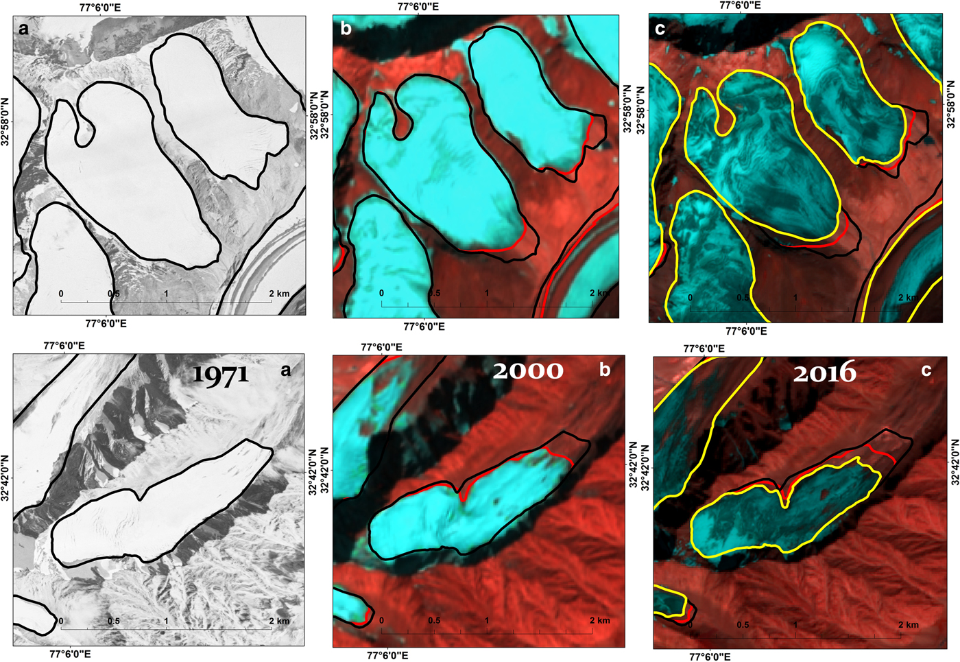
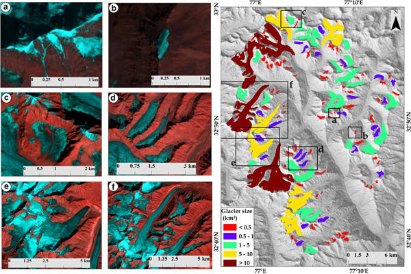
Fig. 3. Satellite images of two sets of glaciers in the Jankar Chhu Watershed, Lahaul Himalaya (see Fig. 1b for location). (a) A rectified subset of Corona image (28 September 1971) based on projective transform and spline method with similar year glacier outline. (b) Coregistered Landsat pan-sharpened ETM+ image (15 October 2000) based on projective transform with Corona and Landsat ETM + glacier outlines. (c) Sentinel 2A image (1 November 2016) with Corona, Landsat ETM+ and Sentinel 2A glacier outlines.
The contiguous ice masses were separated into entities on the basis of the generated watershed (Racoviteanu and others, Reference Racoviteanu, Paul, Raup, Khalsa and Armostrong2009; Schmidt and Nüsser, Reference Schmidt and Nüsser2012), extracted from ASTER GDEM v2 by using the Hydrology Tool in ArcGIS 10.2.2, and further checked and corrected in GE using the 3-D view. The separated glacier areas were transformed to vector data for automatic calculation of glacier size and topographic parameters (e.g. elevation, slope, aspect) (Schmidt and Nüsser, Reference Schmidt and Nüsser2012). The characteristics of glacier distribution were examined by statistically analyzing the relations between topographic parameters and glacier area (Svoboda and others, Reference Svoboda and Paul2009). Each glacier polygon >0.02 km2 was further labelled by corresponding number (Supplementary Figure S1) and categorized as valley, cirque, plateau, hanging, simple (mountain) basin and compound (valley) basin glacier (Supplementary Figure S2) based on Bajracharya and Shrestha (Reference Bajracharya and Shrestha2011) as well as Schmidt and Nüsser (Reference Schmidt and Nüsser2012).
Change detection analyses
For glacier change measurements and quantification, the glacier outlines of 2016 were overlaid on Corona images (1971) as suggested by previous studies (Bolch and others, Reference Bolch, Menounos and Wheate2010a, Reference Bolchb; Bhambri and others, Reference Bhambri, Bolch, Chaujar and Kulshreshtha2011). Overlay adjustments were restricted to the lower part of the analyzed 127 glaciers. The upper accumulation region exhibits no visible changes during the study period (Fig. 3). The area of exposed rocks in the upper section of glaciers was mapped and the calculated area was deducted from the total glaciated area, considering that the ice was lost from these rock faces. For glaciers that fragmented between 1971 and 2016, the combined area was recorded. A bi-temporal comparison between 1971 and 2016 as well as decadal change analyses were carried out for two distinct time span: 1971–2000 and 2000–2016 only for 127 selected glaciers. The rest of the glaciers were obscured by cloud mask on the available Corona images (1971). The Landsat TM scene (1989) had extensive snow cover, and only the glaciers with least seasonal snow cover in the ablation zone were mapped. Therefore, a subset of 41 glaciers out of 127 glaciers was computed for change detection for three distinct time period: 1971–1989, 1989–2000 and 2000–2016. The glacier subset (41) is considered representative as its members are in different size classes between 0.2 and 22.1 km2 (2016) and elevation ranges from 4363 to 6081 m a.s.l.
Mapping uncertainty
Potential errors in this study arise through the image registration, digitization process and with difficulties in correctly identifying the areas of glacier ice. We estimated the mapping uncertainty for each glacier based on a buffer size of 5 m (half of a pixel) for the base image (Sentinel 2A (2016)), and a buffer size of half of the estimated shift (see Table 1: RMSE) caused by misregistration of multi-temporal images to the base image (cf. Granshaw and Fountain, Reference Granshaw and Fountain2006; Bolch and others, Reference Bolch, Menounos and Wheate2010a, Reference Bolchb). This method includes the relative higher error of small glaciers as these have relatively more edge pixels (Bolch and others, Reference Bolch, Menounos and Wheate2010a). Another way to assess the accuracy of glacier boundary extraction via low to medium-resolution images is to compare the extracted boundaries with higher resolution satellite image (Paul and others, Reference Paul, Huggel, Kääb, Kellenberger and Maisch2002, Reference Paul2013). In addition, higher resolution imageries available in GE were taken as reference for accuracy checks. Comparison of outlines for 30 select glaciers derived from Sentinel 2A and GE yields an uncertainty of ±0.9 km2 (~0.6%) (Supplementary Table S1). The final mapping uncertainty was ~2.1% for Sentinel 2A (2016), ~2.4% and ~2.9% for Landsat TM (1989) and pan-sharpened ETM+ (2000) image, respectively, and ~1.2% for Corona (1971). The area change uncertainty was estimated according to standard error propagation, as root sum square of the uncertainty for outlines mapped from different sources (Bhambri and others, Reference Bhambri, Bolch, Chaujar and Kulshreshtha2011). The resultant uncertainties are within the range reported by earlier studies (Bhambri and others, Reference Bhambri, Bolch, Chaujar and Kulshreshtha2011; Paul and others, Reference Paul2013).
RESULTS
Glacier inventory and characteristics
In 2016, 153 glaciers larger than 0.02 km2 were mapped in the study area covering an area of 185.6 ± 3.8 km2 (Table 2a). Of these, 81 glaciers are debris-covered (Table 2a). Morphological type and spatial distribution of glacier size classes are presented in Figure 4. A range of small plateau to large valley glaciers are identified in the JCW, ranging from 0.02 to 21.7 km2 in size (Table 2b; Fig. 5). The mean glacier size (1.2 km2) in the JCW is similar to the other glaciated basins of the Himalayan region, e.g. Ravi (0.6 km2), Shyok (1.4 km2), Ladakh (1 km2), Chenab (1.1 km2), Bhagirathi (1.3 km2), Saraswati/Alaknanda basin (3.7 km2), Ganga (1.1 km2) and Brahmaputra (1.2 km2) (Bhambri and others, Reference Bhambri, Bolch, Chaujar and Kulshreshtha2011; Frey and others, Reference Frey, Paul and Strozzi2012; Schmidt and Nüsser, Reference Schmidt and Nüsser2012; Bajracharya and others, Reference Bajracharya, Maharjan and Shrestha2014; Chand and Sharma, Reference Chand and Sharma2015). Debris-covered ice area in the JCW (~11%) is comparatively lower than the other basins of Western Himalaya (average of all basins ~15%) (Frey and others, Reference Frey, Paul and Strozzi2012). Small glaciers (<1 km2 in size) show a higher percentage (~15%) of debris-covered ice as compared with large glaciers (>5 km2 in size; ~10%) (Table 2a).
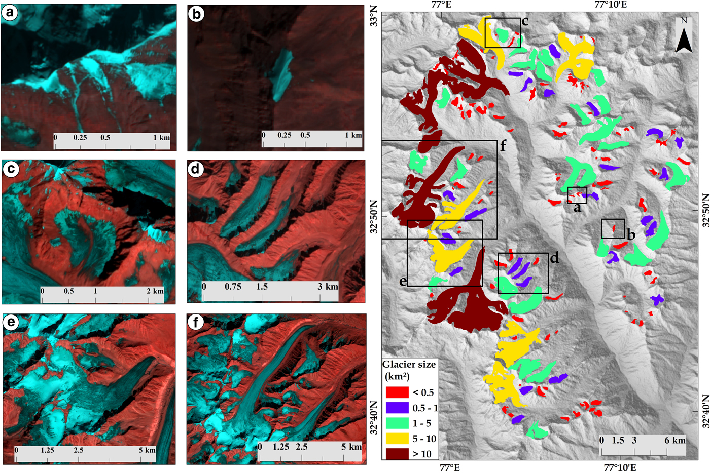
Fig. 4. Glacier types (left) and sizes (right) in the Jankar Chhu Watershed, Lahaul Himalaya in 2016. (a) Hanging glacier with clean ice. (b) Plateau glacier. (c) Cirque glacier with partly debris-covered ice. (d) Simple (mountain) basin glacier with partly debris-covered ice. (e) Compound (valley) basin glacier. (f) Valley glaciers with multiple tributary glaciers and partially debris-covered ice in ablation zone. The background image is Sentinel 2A (12–4–3 bands) (left) and shaded relief map from ASTER GDEM v2 (right).

Fig. 5. Distribution of number of glaciers, glacier area as per size class and morphological type in the Jankar Chhu Watershed. Glacier area and morphological types were derived from Sentinel 2A image (2016) and ASTER GDEM v2.
Compound (valley) basin glaciers have the highest amount of debris-covered ice (~17%), while hanging glaciers are debris-free (Table 2b). In total, 77% of all glaciers have areas <1 km2, covering ~17.5% of the total glacierized area (Table 2a; Fig. 5). Small glaciers (e.g. cirque, plateau and hanging) are dominant in numbers while large glaciers (e.g. valley and mountain basin combinedly) cover ~55.2% of total glacierized area and ~6.6% of all glaciers (Table 2b; Fig. 5).
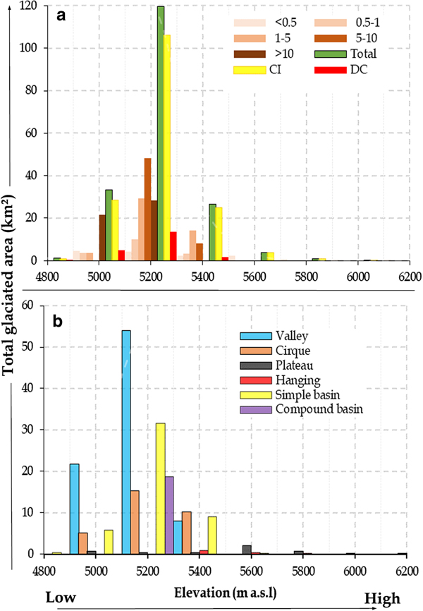
The distribution of glacierized area by elevation (i.e. hypsometry) of total glaciers, clean-ice, debris-covered ice surface, sorted by glacier size classes and according to morphological type is provided in Figure 6. Most of the glaciers in different size classes are distributed between 5200 and 5400 m a.s.l. with smaller glaciers generally at a higher elevation compared with larger glaciers (Table 2a; Fig. 6a). Glaciers >10 km2 in size (ranging from 13.4 to 21.7 km2) are mainly concentrated below 5400 m a.s.l. Valley glaciers are mainly confined below 5400 m a.s.l., while small glaciers (i.e. plateau and hanging) are distributed above 5400 m a.s.l. (Table 2b; Fig. 6b).

Fig. 6. Distribution of glaciated area in relation to altitudinal zones in the Jankar Chhu Watershed. (a) Hypsometry of clean ice (CI), debris-covered ice (DC), total glaciated area (Total) and glaciated area according to different size classes in 2016. (b) Distribution of glacier according to elevation zone and morphological types in 2016. Glacier area and elevation data were derived from Sentinel 2A (1 November 2016) and ASTER GDEM v2.
Mean altitude of glacier ranges from 4843 to 6237 m a.s.l., with an average of 5373 m a.s.l. (Table 2a; Fig. 7a). Mean elevation (~5373 m) of glaciers in the JCW is similar to that of the Central and Western Himalayan basins like Kang Yatze (5710 m), central Ladakh range (5497 m), Alaknanda (5380 m), Bhagirathi (5544 m), Yamuna (5083 m), Sutlej (5436 m), Chenab (5064 m), Indus (5404 m) and Shyok (5868 m) (Frey and others, Reference Frey, Paul and Strozzi2012; Schmidt and Nüsser, Reference Schmidt and Nüsser2017). Elevation range varies according to glacier size class (Table 2; Fig. 7b).
Fig. 7. Scatter plots of (a) glacier size vs mean elevation, (b) glacier size vs elevation range, (c) glacier size vs slope and (d) glacier size vs aspect. Triangle, rhombus, circle, plus, cross and square represent valley, plateau, simple (mountain) basin, cirque, hanging and compound (mountain) basin glacier, respectively. Glacier area and inventory data derived from Sentinel 2A (1 November 2016) and ASTER GDEM v2.
Table 2. Derived glacier parameters (2016) for the Jankar Chhu Watershed based on Sentinel 2A and ASTER GDEM v2
(a) Glacier parameters derived according to size class (km2). (b) Glacier parameters derived according to glaciers type. CI, clean ice; DC, debris-covered ice.
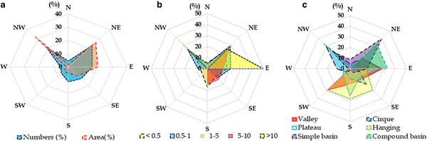
The mean slope of all glaciers is 24° (Table 2a), with smaller glaciers being steeper (Fig. 7c) and the slope of hanging and plateau glaciers is almost twice that of valley glaciers (Table 2b; Fig 7c). Most glaciers (~30%, or ~26% of the area) have northwest aspect (Table 2a; Fig. 8a). Glacier size class distribution according to aspect shows that ~50% of glaciers (>10 km2) are oriented toward the east (Table 2a; Fig. 8b). Valley glaciers are mainly oriented toward the east (~29%) and southwest (~29%), while the maximum number (~87%) of small hanging glaciers are oriented toward the south (Table 2b; Fig. 8c).

Fig. 8. Distribution of glaciers according to aspect in the Jankar Chhu Watershed. (a) Number of the glaciers and glaciated area (%). (b) Number of glaciers (%) in relation to the size class. (c) Number of glaciers (%) in relation to morphological types. Glacier area and elevation data derived from Sentinel 2A (1 November 2016) and ASTER GDEM v2.
Glacier change detection
Glacier area has been lost at heterogeneous rates since 1971 in the JCW (Supplementary Table S2). An example of glacier area change in the JCW is illustrated in Figure 9. During the observation period (1971–2016), glacier area changed from 196.0 ± 2.3 km2 (1971) to 181.4 ± 3.6 km2 (2016), a decrease of 7.5 ± 2.2% (0.2 ± 0.1% a−¹) (Table 3a). The number of analyzed glaciers increased from 127 (1971) to 131 (2016) due to the fragmentation. The loss in glacier area ranged from 1.3 to 52.1% from 1971 to 2016 (Supplementary Table S2). Clean-ice glacier area decreased from 183.4 ± 2.1 km2 (1971) to 161.6 ± 3.2 km2 (2016), a decrease of 11.9 ± 2% (Table 3a). Debris-covered ice increased from 12.6 ± 0.2 km2 (1971) to 19.8 ± 0.4 km2 (2016), an increase of 56.8 ± 3.3% (Table 3a). Out of 127 glaciers, 61 glaciers were covered with debris in 1971 which increased to 76 by 2016 (Table 3a). The spatial distribution map of relative area change indicates that most of the analyzed glaciers lost area below 10% rate between 1971 and 2016 (Fig. 10).

Fig. 9. An example of glacier changes between 1971 and 2016 in the Jankar Chhu Watershed, Lahaul Himalaya (see Fig. 1b for location). Sentinel 2A (12–4–3 bands) image is used as background.
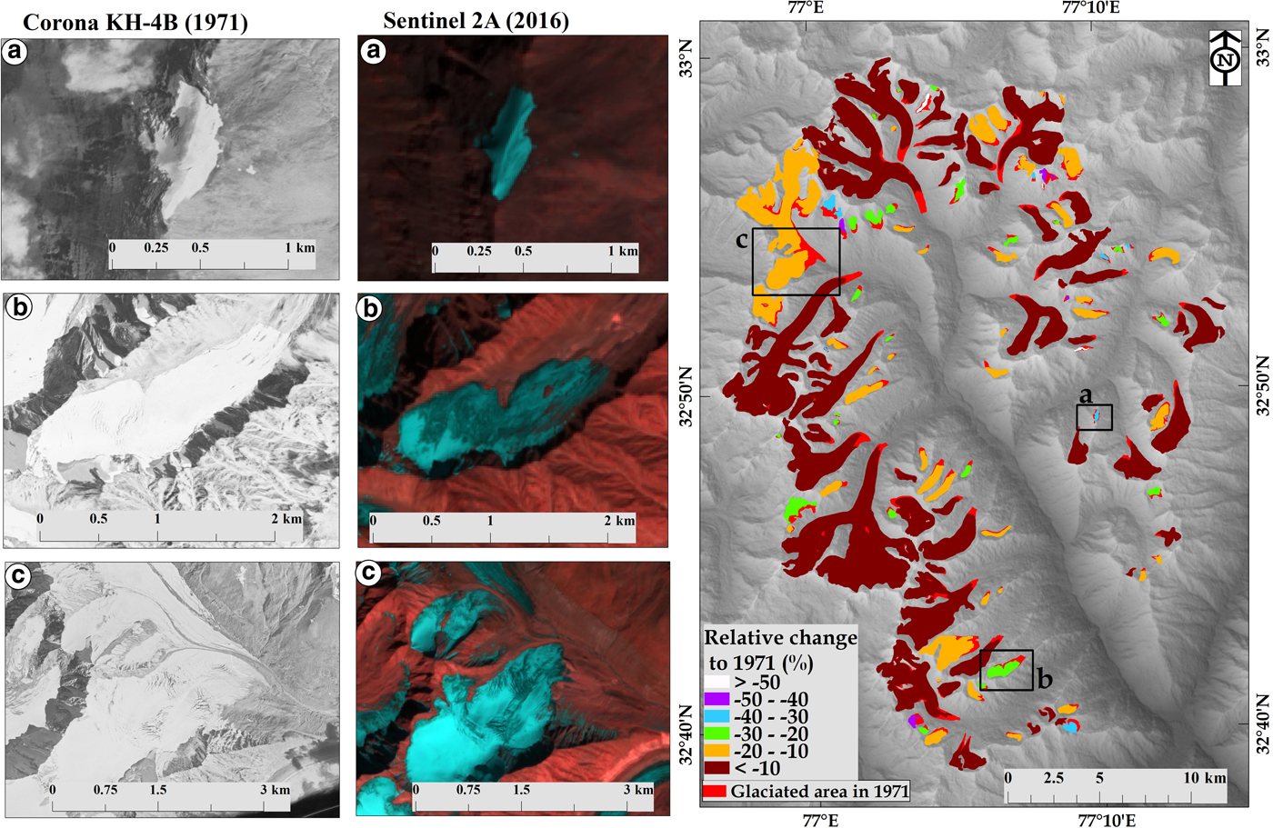
Fig. 10. Map of relative glacier area change (%) between 1971 and 2016 in the Jankar Chhu Watershed (right panel). Satellite images of three sets of glaciers showing surface area change between 1971 (Corona) and 2016 (Sentinel 2A) (left panel).
Table 3. Changes in total ice area, clean ice (CI) area and debris-covered (DC) ice area in the Jankar Chhu Watershed, Lahaul Himalaya between 1971 and 2016 based on satellite remote-sensing data
(a) Change detection for 127 mapped glaciers in 1971. (b) Change detection for 41 mapped glaciers in 1989.
Decadal glacier area change was examined in detail for 41 mapped glaciers (1989) (Table 3b). These glaciers (41) lost 2.2 ± 3.9 km2 (1.3 ± 2.4 or 0.1 ± 0.1% a−¹) of their area from 1971 to 1989, 2.4 ± 5.2 km2 (1.5 ± 3.2 or 0.14 ± 0.3% a−¹) from 1989 to 2000 and 4.8 ± 4.6 km2 (3.0 ± 2.9 or 0.2 ± 0.1% a−¹) from 2000 to 2016. Analysis indicates that glacier recession has slightly increased in recent decades (2000–2016) as compared with 1971–1989 (Table 3b).
Glaciers between 0.5 and 1 km2 in size lost maximum area (21.3 ± 2 or 0.5 ± 0.1% a−¹) from 1971 to 2016 (Table 4; Fig. 11a). Glaciers >10 km2 in size witnessed minimum area loss of 3.0 ± 1.5 km2 (4.6 ± 2.2 or 0.1 ± 0.1% a−¹) mainly due to lowest mean elevation (i.e. comparatively lower terminus elevation) and highest percentage of clean-ice area (89.35%) in 2016 (Table 4; Fig. 11a). Change in small glaciers is higher than valley glaciers, not ignoring the fact that earlier image database had snowdrift accumulation in the higher region. In absolute term, large glaciers lost more area than small glaciers (Fig. 11b). Relative area change according to morphological categories is interpreted in Table 5.

Fig. 11. Scatter plots of (a) glacier size (km2) vs glacier area change (%), (b) glacier size (km2) vs glacier area change (km2), (c) mean slope vs glacier area change (%), (d) aspect vs glacier area change (%), (e) mean elevation vs glacier area change (%) and (f) elevation range vs glacier area change (%) for 127 analyzed glaciers. Triangle, rhombus, circle, plus, cross and square represent valley, plateau, simple (mountain) basin, cirque, hanging and compound (mountain) basin glacier, respectively.
Table 4. Area loss according to glacier size class from 1971 to 2016 in the Jankar Chhu Watershed
Table 5. Area loss according to glacier morphological type between 1971 and 2016 in the Jankar Chhu Watershed
Glaciers with southward aspect (including southeast, south and southwest) have decreased by 21.2 ± 2.2 or 0.5 ± 0.1% a−¹, while glaciers with northward aspect (including north, northeast and northwest) have receded by 13.7 ± 1.8 or 0.3 ± 0.01% a−¹ between 1971 and 2016 (Fig. 11d). In addition, glaciers with the west and east aspect have lost their area by 15.1 ± 1.9 or 0.3 ± 0.01% a−¹ (Fig. 11d). Area change rate is almost twice the rate for glacier above 5400 m a.s.l. as compared with those below 5400 m a.s.l. (Table 6; Fig. 11e). The glaciers above 500 m elevation range receded at a lower rate as compared with others (Fig. 11f).
Table 6. Glacier area loss according to elevation zones between 1971 and 2016 in the Jankar Chhu Watershed
Climatic trends
In the absence of availability of long-term climatic data within the JCW, we analyzed available grided temperature data based on US National Center for Environmental Prediction/National Center for Atmospheric Research (NCEP/NCAR) reanalysis data between 1948 and 2017 (see Kalnay and others, Reference Kalnay1996). Temperature (°C) trend was analyzed for the grid (32.5°N and 77.5°E) located within the JCW based on Mann–Kendall method (Bhambri and others, Reference Bhambri, Bolch, Chaujar and Kulshreshtha2011; Negi and others, Reference Negi, Saravana, Rout and Snehmani2013; Chand and Sharma, Reference Chand and Sharma2015) (Supplementary Table S3). The mean annual temperature (MAT) showed an insignificant increasing trend (0.0078 °C a−¹) from 1948 to 2017 (Fig. 12), but the MAT increases significantly between 1997 and 2016. Winter (December, January, February: DJF) mean temperature increased significantly by ~1.3 °C for the selected grid while summer (March, April, May: MAM) mean temperature decreased by ~0.2 °C between 1948 and 2017 (Supplementary Table S3).
Fig. 12. Trends in mean annual temperature (°C) between 1948 and 2017 for the part of Lahaul Himalaya (32.5°N and 77.5°E grid within the JCW) based on US National Center for Environmental Prediction/National Center for Atmospheric Research (NCEP/NCAR) reanalysis I datasets at 2.5° × 2.5° spatial resolution. Data source: NCEP reanalysis data provided by the NOAA/OAR/ESRL PSD, Boulder, Colorado, USA, and downloaded from their website (https://www.esrl.noaa.gov/psd/).
DISCUSSION
Comparison with RGIv6.0/GAMDAM and ICIMOD
For comparison and cross-check, vector shapefile derived from: (i) glacier outlines of RGIv6.0/GAMDAM (2000 ± 3) and (ii) ICIMOD (2008 ± 3) were overlaid with the outlines derived from Sentinel 2A (2016). A comparison of our results with those published by RGIv6.0 using the data from GAMDAM inventory (Nuimura and others, Reference Nuimura2015) indicated that glacier area in the JCW was overestimated (~6.7 km2 or ~4%), while glacier number was underestimated (11 or ~8%) by RGIv6.0/GAMDAM (Supplementary Table S4). Ironically, in the revised version of GlobGlacier inventory (RGI v6), the number of glaciers in the JCW had shown a significant decrease (~27.92%) from its earlier version (RGI v4). The ICIMOD glacier inventory contains 145 glaciers covering an area of ~177.3 km2 with similar minimum size (0.02 km2). Interestingly, in the present analysis, we obtained more glaciers (8 or ~6%) as well as a larger glacierized area (~8.26 km2 or ~5%) a decade later in 2016 (Supplementary Table S4). We suggest that this variation is attributed to (i) misinterpretation of debris-free and debris-covered glaciers; (ii) temporal differences in terms of acquired images and mapping period; (iii) differences in classification of glacier area/boundary; and (iv) adjacent ice masses may have been clumped as a single entity (Supplementary Figure S3). In addition, Birajdar and others (Reference Birajdar, Venkataraman, Bahuguna and Samant2014) have generated a glacier inventory of Bhaga basin for 2011 using Indian remote-sensing linear imaging self-scanning sensor (LISS III) data and the ASTER GDEM at 1:50 000 scale which is not freely available (Supplementary Table S4). The Geological Survey of India (GSI) also attempted a glacier inventory based on the SoI topographic maps, aerial photographs and satellite images for the Indian Himalaya (Raina and Srivastava, Reference Raina and Srivastava2008).
Comparison of area change within Chenab basin
The present study indicates that glacier recession rate in the JCW (0.17 ± 0.01% a−¹) from 1971 to 2016 is less than reported for Chenab basin. Our study shows an apparently lower retreat rate compared with the analyses using SoI maps derived glacier boundary (Kulkarni and Alex, Reference Kulkarni and Alex2003; Kulkarni and others, Reference Kulkarni2007, Reference Kulkarni2010; Sharma and others, Reference Sharma2016; Brahmbhatt and others, Reference Brahmbhatt2017) (Supplementary Table S5). For instance, glaciers in the Bhaga basin retreated at ~0.8% a−¹, in Chenab at ~0.5% a−¹, in Miyar at ~0.2% a−¹, in Warwan at ~0.5% a−¹ between 1962 and 2001/04 (Kulkarni and others, Reference Kulkarni2007; Kulkarni, Reference Kulkarni2010) (Supplementary Table S5). Kulkarni and others (Reference Kulkarni, Dhar, Rathore, Govindha and Kalia2006) showed that Samudra Tapu glacier (source of Chandra River) retreated by 11% or ~0.3% a−¹ between 1962 (SoI maps) and 2000 (LISS III images). In Warwan-Bhut region of Chenab basin, Brahmbhatt and others (Reference Brahmbhatt2017) reported area loss of 11% (~0.3% a−¹) based on SoI maps (1962) and LISS III (2001) images. The higher rate of glacier retreat could be a result of an overestimation of glacier cover in the SoI maps as reported by previous studies (Bhambri and others, Reference Bhambri, Bolch, Chaujar and Kulshreshtha2011; Chand and Sharma, Reference Chand and Sharma2015). Negi and others (Reference Negi, Saravana, Rout and Snehmani2013) noted higher retreat rate (~0.4 ± 0.1% a−¹) for small Baralacha glacier in Bhaga basin between 1971 and 2010 using Corona, Landsat and LISS IV images (Supplementary Table S5).
Our analysis of glacier area change for the JCW also confirms published trends as reported by Pandey and Venkataraman (Reference Pandey and Venkataraman2013) and Birajdar and others (Reference Birajdar, Venkataraman, Bahuguna and Samant2014) (Supplementary Table S5). Birajdar and others (Reference Birajdar, Venkataraman, Bahuguna and Samant2014) observed retreat rate of 0.16 ± 0.1% a−¹ in Bhaga basin from 2001 to 2011 which is similar to our result (0.17 ± 0.01% a−¹). In line with our assumption and data, Pandey and Venkataraman (Reference Pandey and Venkataraman2013) also reported similar retreat rate of ~0.1% a−¹ for the 15 selected glaciers in Chandrabhaga basin (1980–2010), using exclusively remotely sensed datasets. In adjacent Miyar basin, Patel and others (Reference Patel, Sharma, Fathima and Thamban2018) observed similar retreat rate (~0.16% a−¹) (Supplementary Table S5). Based on satellite imagery, Garg and others (Reference Garg, Shukla, Tiwari and Jasrotia2017a) reported lower retreat rate for Sakchum (~0.15% a−¹), Chhota Shigri (~0.06% a−¹) and Bara Shigri (~0.04% a−¹) glaciers in upper Chenab basin between 1993 and 2014 (Supplementary Table S5).
Comparison of area change with other Himalayan basins
Glacier area change studies carried out across the Himalaya have been given in Supplementary Table S5. In Western Himalaya (1962–2001), glaciers retreated at higher rate than the present study (Kulkarni and others, Reference Kulkarni2007; Kulkarni, Reference Kulkarni2010; Schmidt and Nüsser, Reference Schmidt and Nüsser2012; Chudley and others, Reference Chudley, Miles and Willis2017). Based on Corona and Landsat images, Chand and Sharma (Reference Chand and Sharma2015) recorded much lower retreat rate (~0.1 ± 0.1% a−¹) in Ravi basin of Himachal Himalaya. In Garhwal Himalaya, Bhambri and others (Reference Bhambri, Bolch, Chaujar and Kulshreshtha2011) reported similar retreat rate to the present one (Supplementary Table S5). Bolch and others (Reference Bolch, Buchroithner, Pieczonka and Kunert2008) stated glacier area loss by 5.2% (~0.12% a−¹) in the Kumbhu Himalaya. For Bhutan Himalaya, Bajracharya and others (Reference Bajracharya2015) showed higher retreat rate between 1980 and 2010 derived using Landsat images (Supplementary Table S5).
Potential reason for debris cover increase
Several studies have indicated that the debris-covered area has increased on glacier surface over time, and such glaciers show a lower rate of recession as compared with clean glaciers in the Himalaya (Bolch and others, Reference Bolch, Buchroithner, Pieczonka and Kunert2008; Bhambri and others, Reference Bhambri, Bolch, Chaujar and Kulshreshtha2011; Kamp and others, Reference Kamp, Byrne and Bolch2011; Chand and Sharma, Reference Chand and Sharma2015). The present study also confirms that the number as well as area of debris-covered glaciers has increased by 15 and 7.2 ± 3.8 km2 (~0.16 ± 0.1 km2 a−¹), respectively, between 1971 and 2016, probably due to the melting of clean-ice surface resulting in the exposure of debris-cover surface. Different spatial resolution (Corona: 2 m; Sentinel 2A: 10 m) as well as time gap of image acquisition (Corona: 28 September 1971; Sentinel 2A: 1 November 2016; 33 day gap) may lead to overestimation of debris-covered ice area in the JCW, not ignoring the role of local weather regime in such complex terrain. In Bhutan Himalaya, Nagai and others (Reference Nagai, Fujita, Nuimura and Sakai2013) observed a significant correlation between the surface area of southwest facing potential debris supply (PDS) slopes and debris-covered area with a maximum contribution of debris mantle from the southwest facing PDS slopes. To investigate whether this relation of debris cover exists in the JCW, we demarcated the distribution of PDS slope for the glaciers which have more than 10% of debris-covered area to the total area (Supplementary Figure S4). It is found that 50% of PDS slope for these glaciers (>10% of debris-covered area) is in the south (including south, southeast and southwest) facing. A similar pattern is also reported in the Ravi basin, northwestern Himalaya (Chand and Sharma, Reference Chand and Sharma2015). Thus, the suggested explanation of debris supply from PDS slope surrounding the glaciers might apply for the JCW too. Several studies have emphasized the significance of supraglacial debris cover on the glacier dynamics in response to climate change whereby modifying surface ablation rates and spatial patterns of mass loss (Benn and Lehmkuhl, Reference Benn and Lehmkuhl2000; Scherler and others, Reference Scherler, Bookhagen and Strecker2011a; Dobhal and others, Reference Dobhal, Mehta and Srivastava2013; Pratap and others, Reference Pratap, Dobhal, Mehta and Bhambri2015). In addition, experimental and short-period (ablation season) studies suggest that thick debris cover reduces ablation, whereas thin debris layer increases ice melt underneath (Pratap and others, Reference Pratap, Dobhal, Mehta and Bhambri2015). Debris-covered ice in the JCW is mainly confined to large valley glaciers where terminus fluctuation may have been affected by the supraglacial debris cover.
Influence of non-climatic factors on glacier fluctuations
Since 2000, the rate of recession has increased in the JCW of Lahaul Himalaya. A similar trend in glacier recession has been reported in the Gharwal Himalaya (Bhambri and others, Reference Bhambri, Bolch, Chaujar and Kulshreshtha2011) and in the Kumbhu Himalaya (Bolch and others, Reference Bolch, Buchroithner, Pieczonka and Kunert2008). The number of glaciers increased by four in the JCW between 1971 and 2016, which we attribute to glacier fragmentation. A similar trend has been reported in the other basins of Western Himalaya (Kulkarni and others, Reference Kulkarni2007; Chand and Sharma, Reference Chand and Sharma2015) and Central Himalaya (Bhambri and others, Reference Bhambri, Bolch, Chaujar and Kulshreshtha2011).
In the JCW, glaciers <1 km2 in size have lost 14.3 ± 2.1% (~0.3 ± 0.1% a−¹) of area from 1971 to 2016, whereas in similar basin (e.g. Chenab) Kulkarni and others (Reference Kulkarni2007) found that glaciers <1 km2 in size lost 38% (~1% a−¹) of area between 1962 (SoI maps) and 2001/04. We observed a negative correlation (r = −0.4) between glacier size and relative surface area change while the absolute area change showed a significant positive correlation (r = 0.7) with glacier size by simple linear regression (Figs 11a, b). It is difficult to ascertain the reason whether the elevation or little accumulation area is a factor for the rapid recession of small glaciers in the JCW. Our results show that small glaciers receded at a faster rate than large glaciers in the JCW. Many studies have already highlighted that smaller glaciers are characterized by a higher rate of decrease in area as compared with larger glaciers (Bolch and others, 2010; Bhambri and others, Reference Bhambri, Bolch, Chaujar and Kulshreshtha2011; Schmidt and Nüsser, Reference Schmidt and Nüsser2012; Negi and others, Reference Negi, Saravana, Rout and Snehmani2013; Chand and Sharma, Reference Chand and Sharma2015).
The north facing (including north, northwest and northeast) glaciers receded less than the south (including south, southwest and southeast) facing ones in the JCW (Fig. 11d). It may be due to less radiation received by the northern slopes than the south facing Himalayan slopes (Scherler and others, Reference Scherler, Bookhagen and Strecker2011b). Thus the north facing glaciers are likely to have responded slowly than the south facing ones in the JCW. Whether such a response is to be related to reduce precipitation is not readily recognized.
Glaciers with lower mean elevation receded less than the glacier in higher elevation. We found very low positive correlation (r = 0.2) between mean elevation (m a.s.l.) and glacier area change (%) while elevation range (m) exhibited significant negative correlation (r = −0.5) (Figs 11e, f), indicating that elevation range is more influential factor for glacier surface area loss as compared with mean elevation in the JCW. Glacier morphology (e.g. shape, size and hypsometry), steep slope and small accumulation area may accelerate the retreat rate of glaciers on higher elevations in such region (Salerno and others, Reference Salerno2017; Garg and others, Reference Garg, Shukla and Jasrotia2017b), not ignoring the fact that large valley glaciers have longer response times.
Potential climatic controls on glacier fluctuations
The analysis of NCEP/NCAR data shows that MAT within the JCW region increased by ~0.5 °C between 1948 and 2017. Negi and others (Reference Negi, Saravana, Rout and Snehmani2013) reported that MAT increased by ~2.2 °C (~0.07 °C a−¹) and winter snowfall decreased by ~242.1 cm (8.3 cm a−¹) for Patsio between 1983 and 2011. Shehmani and others (Reference Shehmani, Dharpure, Kochhar, Ram and Ganju2015) noted decreasing mean seasonal snowfall (0.07 cm a−¹) in Bhaga basin during 2001–12. Shekhar and others (Reference Shekhar, Chand, Kumar, Srinivasan and Ganju2010) have reported an increase of 2.8°C in annual maximum temperature (T MAX) between 1984/85 and 2007/08 in the Western Himalaya; while minimum temperature (T MIN) increased by ~1°C during the similar period. Dash and others (Reference Dash, Jenamani, Kalsi and Panda2007) also mentioned that T MIN decreased by 1.9°C over the Western Himalaya during 1955–72 and increasing trend in last decades. Bhutiyani and others (Reference Bhutiyani, Kale and Pawar2010) had reported the annual warming rate of 1.6°C over the last century with a significant increase of ~3.2°C in winter average T MAX. In addition, summer cooling has been reported in some part of the Western Himalaya and upper Indus basin during the last two decades of the 20th century (Yadav and others, Reference Yadav, Park, Singh and Dubey2004; Bhutiyani and others, Reference Bhutiyani, Kale and Pawar2007; Rajbhandari and others, Reference Rajbhandari, Shrestha, Kulkarni, Patwardhan and Bajracharya2014). Our analysis of NCEP/NCAR reanalysis data also suggests strong warming trends in winter and weaker cooling in summer, suggesting a lower annual variability which is one of the regional causes of glacial waning. Bhutiyani and others (Reference Bhutiyani, Kale and Pawar2010) also described significant decreasing trends in the monsoon precipitation during the period 1866–2006. Shekhar and others (Reference Shekhar, Chand, Kumar, Srinivasan and Ganju2010) reported a decrease in total seasonal snowfall of ~280 cm over the entire Western Himalaya and ~440 cm in the Greater Himalaya range between 1988/89 and 2007/08 which appears to be factually incorrect and extraordinary inflated value. They have taken only two time periods of data and not of continuous years. However, Shehmani and others (Reference Shehmani, Dharpure, Kochhar, Ram and Ganju2015) support our field observation and reality. The field region is being visited twice a year, pre- and post-monsoon since 2003. Snow and glacier conditions (e.g. available snowfields, avalanche cones and amount of meltwaters) are recorded accordingly on either of the field visits.
Based on climatic trends identified from NCEP/NCAR data and existing studies, it might be argued that loss of glacier surface area in the JCW between the 1970s and 2016 reflects the combined influence of rising temperature and declining precipitation. Since 1950–1990, MAT showed negative trend, while in recent decades (1990–2017), MAT increased at a significant rate (Fig. 12). In the present study, we had higher area loss rate (~0.2 ± 0.02% a−¹) in recent decades (2000–16) as compared with previous decades (~0.1 ± 0.01% a−¹; 1971–2000). Higher deglaciation in recent decades may be attributed to increasing trend in MAT as well as decreasing trend in precipitation as reported elsewhere. The availability of long-term instrumental climatic records and field-based measurements (e.g. mass balance, debris cover thickness) within the watershed will provide a valuable database and further improve knowledge of glacier change and its interaction/response to ongoing changes in climatic parameters in the JCW of Lahaul Himalaya.
CONCLUSION
This study provides a comprehensive multi-temporal glacier fluctuations record for the JCW, Chandrabhaga basin, Lahaul Himalaya between 1971 and 2016. Glacier area decreased by 14.7 ± 4.3 km2 (0.3 ± 0.1 km2 a−¹) from 1971 to 2016. Glaciers lost less area (0.1 ± 0.1% a−¹) during 1971–2000 than 2000–2016 (0.2 ± 0.2% a−¹). Debris cover increased by 7.2 ± 0.4 km2 (~0.2 ± 0.01 km2 a−¹) between 1971 and 2016. Glacier recession rate is comparatively lower in the JCW than other basins of Western Himalaya (e.g. Chenab, Beas, Miyar, Parbati, Tirungkhad and Baspa). Smaller glaciers (<1 km2) lost 14.3 ± 2.1% of ice, while glaciers >10 km2 in size lost 4.6 ± 2.2%, which is a common trend between glacier size and average shrinkage rate. Glaciers with south aspect shrank at a faster rate than glacier with other aspects. The influence of topographical factors on glacier change rates needs to be studied with respect to the response of the glacier to ongoing changes in climatic parameters.
SUPPLEMENTARY MATERIAL
The supplementary material for this article can be found at https://doi.org/10.1017/jog.2018.77.
ACKNOWLEDGEMENTS
S. Das is thankful to the University Grant Commission, New Delhi (3090/ (NET–DEC.2014) for financial support during field observations. We also thank USGS for providing Sentinel 2A, Landsat and Corona data at no cost. We acknowledge the DST–CCP/SPLICE (IUCCCC) for supporting field comparing and laboratory facilities. Hester Jiskoot and Neil Glasser are thanked for constructive comments of the paper. We also thank two anonymous referees for their insightful suggestions, which considerably improved the earlier version of the manuscript.


 Open access