


1. INTRODUCTION
Retreating mountain glaciers around the world have become icons of anthropogenic climate change. These glaciers are important regulators of seasonal water availability in many regions (e.g., Immerzeel and others, Reference Immerzeel, Pellicciotti and Bierkens2013; Rangecroft and others, Reference Rangecroft2013; Huss and Hock, Reference Huss and Hock2018), and both growing and shrinking glaciers may cause geohazards (e.g., Richardson and Reynolds, Reference Richardson and Reynolds2000; Kääb and others, Reference Kääb2018) and transform existing landscapes (Haeberli and others, Reference Haeberli, Schaub and Huggel2017). On a global scale, the glaciers outside the Antarctic and Greenland ice sheets, but including those in the periphery of the ice sheets (henceforth referred to as glaciers) cover an area of 706 000 km2 (RGI Consortium, 2017). Despite making up <1% of the Earth's global land ice volume (~0.4 m sea-level equivalent (SLE) compared to 65.7 m SLE contained in the Antarctic and Greenland ice sheets (Vaughan and others, Reference Vaughan2013), these glaciers contribute significantly to current global sea-level rise.
Meier (Reference Meier1984) was one of the first to recognize the role of glaciers in the 20th-century sea-level budget, concluding that they may have contributed a third to half of observed sea-level rise between 1884 and 1975. A contribution of 20–30% was estimated by Kaser and others (Reference Kaser, Cogley, Dyurgerov, Meier and Ohmura2006) for the period 1991–2004 extrapolating mass-balance data from the sparse network of direct glaciological measurements (e.g., Dyurgerov and Meier, Reference Dyurgerov and Meier2005) to the global scale. Gardner and others (Reference Gardner2013) combined direct glaciological data with mass change estimates derived from geodetic and gravimetric data and estimated a sea-level contribution from glaciers of 259 ± 28 Gt a−1 (0.71 ± 0.08 mm SLE a−1 or ~30% of observed sea-level rise) between October 2003 and October 2009. This estimate is similar to the one for both ice sheets combined (289 ± 49 Gt a−1, 0.80 ± 0.14 mm SLE a−1) for roughly the same period (2000–2011; Shepherd and others, Reference Shepherd2012). A recent update by Zemp and others (2019) based on analyses of glaciological and geodetic observations found a global glacier sea-level contribution of 335 ± 144 Gt a−1 (0.92 ± 0.39 mm SLE a−1) for the period 2006–2016. Glaciers are expected to remain an important contributor to sea-level rise during the 21st century (Meier and others, Reference Meier2007; Church and others, 2013), and any attempts to close the sea-level budget of the past and coming decades/centuries need to include the contribution from glaciers outside the ice sheets. Hence, it is essential to develop adequate predictive tools of the glaciers' response to climate variability at a global scale.
This study is part of GlacierMIP (Glacier Model Intercomparison Project), a so-called Targeted Activity by the ‘Climate and Cryosphere’ (CliC) project of the World Climate Research Project (WCRP). GlacierMIP provides a framework for a coordinated intercomparison of global-scale glacier evolution models with the ultimate goal of advancing our understanding of past and future glacier changes and their contribution to sea-level rise on a global scale. The specific objectives are: (1) to coordinate a model intercomparison of existing global-scale glacier models with respect to century-scale glacier mass change projections; (2) to identify current model deficiencies and data needs; and (3) to work towards a new generation of global-scale glacier models and define community-based standardized experiment design and forcing data, to improve simulations of global glacier changes.
A number of community-organized model intercomparison projects for land ice have been undertaken during the last decades, but these have focused almost entirely on ice-sheet modeling, for example the Ice Sheet Model Intercomparison project (ISMIP) for Higher-Order ice-sheet Models (ISMIP-HOM, Pattyn and others, Reference Pattyn2008), the Marine ISMIP (MISMIP, Pattyn and others, Reference Pattyn2012), model intercomparisons within the European Ice Sheet Modelling Initiative (EISMINT, Huybrechts and Payne, Reference Huybrechts and Payne1996; Payne and others, Reference Payne2000; Saito and others, Reference Saito, Abe-Ouchi and Blatter2006), the Sea-level Response to Ice Sheet Evolution project (SeaRISE, Bindschadler and others, Reference Bindschadler2013; Nowicki and others, Reference Nowicki2013a, Reference Nowickib) and the ISMIP6 (Nowicki and others, Reference Nowicki2016). As part of EISMINT, Oerlemans and others (Reference Oerlemans1998) compared the mass evolution of selected mountain glaciers and ice caps to standardized forcing scenarios, however, the suite of glacier models was only compared for 12 glaciers. No coordinated effort has been made so far to compare global-scale glacier models and their projections in a comprehensive and systematic manner.
In fact, compared to the abundance of models for ice sheets, only a few models capable of modeling glaciers on a global scale have been reported in the literature (see Radić and Hock, Reference Radić and Hock2014 for a review). Until recently such modeling was hampered by lack of fundamental inventory data (Radić and Hock, Reference Radić and Hock2010), requiring authors to adopt highly simplified approaches and to extrapolate results to uninventoried areas. The few published studies prior to 2011 typically adopted a sensitivity approach to model global mass changes over time (Zuo and Oerlemans, Reference Zuo and Oerlemans1997; Gregory and Oerlemans, Reference Gregory and Oerlemans1998; Raper and Braithwaite Reference Raper and Braithwaite2006) modeled glacier mass balances on a 1° × 1° grid based on mass-balance profiles derived from temperature-index melt modeling, but glacier-size distributions and results had to be upscaled to cover all glaciers in the world. Radić and Hock (Reference Radić and Hock2011) were the first to model every single glacier for which inventory data were available (~40% of global glacier area) using a temperature-index melt model forced by transient climate data. However, even here, large uncertainties still stemmed from the need to upscale results to uninventoried glacier areas.
The recently completed Randolph Glacier Inventory (RGI, Pfeffer and others, Reference Pfeffer2014; RGI Consortium, 2017), which for the first time provided basic inventory data for all ~200,000 glaciers in the world, opened new opportunities for more sophisticated approaches to model glaciers on a global scale. Since the release of its first version in 2012, results from six distinct models have been published which used the RGI data to make projections of all the glaciers in the world driven by transient climate scenarios until the end of the 21st century (Tables 1, 2).
Table 1. Characteristics of the glacier models used in the intercomparison of global-scale glacier projections. The models are referred to by the short name given in the second row. Where available we use the model names given in the original literature (marked in italic). Studies are ordered according to the year of publication. See text (Section 3) for further details

V = glacier volume, A = glacier area, L = glacier length.
Table 2. Characteristics of model input data used by the six glacier models that are compared in this study. N is the number of model runs. For three models (SLA2012, MAR2012, GIE2013) we use model output that has been updated compared to the original publications using more recent inventory and/or climate datasets (see text)

a Here we use the re-calculated results from Bliss and others (Reference Bliss, Hock and Radić2014); differences are negligible.
b Fifth Assessment Report of the Intergovernmental Panel on Climate Change (IPCC).
c Climate Research Unit.
d Global Climate Model output from the Fifth Coupled Model Intercomparison Project.
e European Reanalysis by the European Centre for Medium-Range Weather Forecasts.
f Dataset prepared by Global Precipitation Climatology Centre, German Climate Research Programme (DEKLIM).
g In the original publication CMIP3 data were used.
h World Glacier Inventory – Extended Format.
i In the original publication RGI v1.0 was used.
This study presents the first activity within GlacierMIP, which aims to systematically compare recently published global-scale glacier model results in order to foster model improvements and reduce uncertainties in global glacier projections. Specifically, we investigate output from six glacier models between 2015 and 2100 by comparing the models' projected glacier mass and area changes, and their corresponding sea-level contributions, both globally and for each of the RGI's 19 primary glacier regions (Fig. 1).
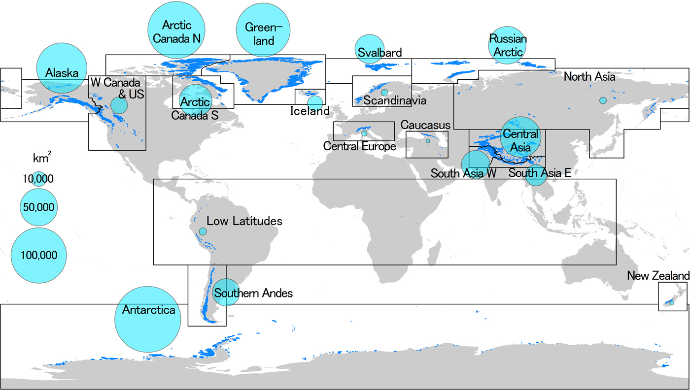
Fig. 1. Global distribution of glaciers (dark blue) subdivided into 19 regions (black boxes). Light blue circles indicate each region's glacier area in km2. Region boundaries and names are from the Randolph Glacier Inventory (RGI). Areas refer to those modeled by the six glacier models on average for year 2015 (Supplementary Table S2).
2. DATA AND METHODS
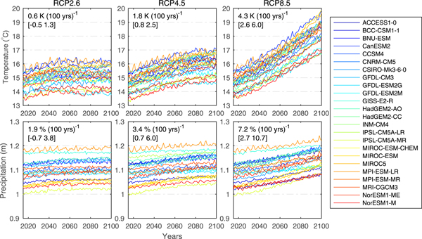
In response to an open call for data, six modeling groups submitted their annual glacier mass and area evolution projections to GlacierMIP. The data are available in the Supplementary Material. The models will hereafter be referred to either by the model acronyms introduced by the authors (GloGEM, HYOGA2), or, when no name was provided (four models), by abbreviations based on the most relevant reference (first three letters of first author's name followed by the publication year, Table 1). The six studies forced their glacier model with projections from 8 to 21 General Circulation Models (GCMs) from the fifth phase of the Coupled Model Intercomparison Project (CMIP5; Taylor and others, Reference Taylor, Stouffer and Meehl2012) and several emission scenarios (Tables 1, 2, Supplementary Table S1). Here we analyze the data from all available individual model runs (in total 214) forced by Representative Concentration Pathways RCP2.6, RCP4.5, RCP6.0 and RCP8.5 (van Vuuren and others, Reference van Vuuren, Edmonds and Kainuma2011). We note that most glacier models do not use all four RCPs. These emission scenarios describe a range of radiative forcing pathways and are named after radiative forcing relative to pre-industrial values (+2.6, +4.5, +6.0 and +8.5 W m−2) reached before year 2100 (RCP2.6, RCP4.5), beyond 2100 (RCP6.0), and ~2100 (RCP8.5). Globally-averaged projections of near-surface temperature and precipitation of all GCMs used in this study are shown in Figure 2.
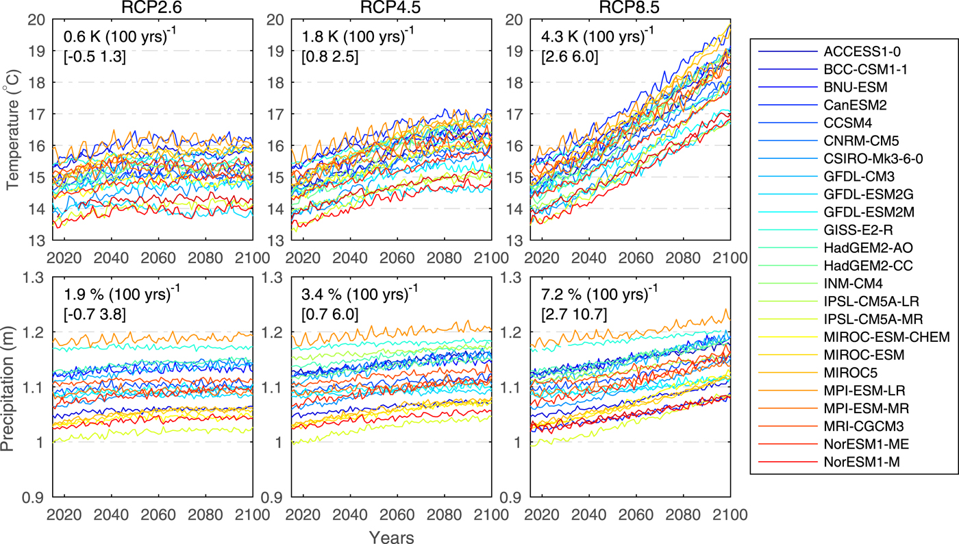
Fig. 2. Globally averaged annual mean near-surface air temperature and annual precipitation for the period 2015–2100 projected by the 25 GCMs used for the glacier modeling. Time series are shown for three emission scenarios (RCPs). Numbers in subplots refer to temperature and precipitation changes over the 86-year period expressed in K (100 a−1) and % (100 a−1), respectively, averaged over all GCMs. Minimum and maximum values are given in brackets.
In total 25 GCMs were used in the six modeling studies, but only four GCMs (CNRM-CM5, MRI-CGCM3, MPI-ESM-LR, NorESM1-M) were used by all six glacier models (Supplementary Figure S1). Three of the 25 GCMs were only used by one of the six glacier models (GIE2013). Most glacier model runs are available for RCP8.5 (88 out of 214 runs). Since only two studies used the RCP6.0 scenario (16 runs), we focus primarily on the results of the RCP2.6, RCP4.5 and RCP8.5 results. All GCM projections refer to the ‘r1i1p1’ model ensemble member.
For three models (MAR2012, SLA2012, GIE2013) the data analyzed here refer to updated results compared to the original publications (Table 2). SLA2012 and GIE2013 were re-run using CMIP5 rather than CMIP3 projections, which were used in Slangen and others (Reference Slangen, Katsman, van de Wal, Vermeersen and Riva2012) and Giesen and Oerlemans (Reference Giesen and Oerlemans2013). MAR2012 was rerun with updated input data (RGI 4.0 instead of RGI 1.0, RGI's elevation data, Climate Research Unit (CRU) temperature and precipitation data updated to TS 3.22 instead of TS3.0 compared to Marzeion and others (Reference Marzeion, Jarosch and Hofer2012)). Updated results for MAR2012 and SLA2012 are also shown in Slangen and others (Reference Slangen, Adloff, Jevrejeva, Leclercq, Marzeion, Wada and Winkelmann2017).
Huss and Hock (Reference Huss and Hock2015) report results for both a temperature-index and a simplified energy-balance model within GloGEM, but here we only analyze results from the former approach. Modeling periods varied between the studies (Table 2). Here we focus on century-scale projections and analyze the data from 2015 to 2100. Two models lack data for the last year (GIE2013) or last 5 years (SLA2012) of the 21st century, so we extrapolate the glacier mass time series using the rate of change of the preceding 5 years. Each model used slightly different values for the ocean area (360.0 × 10⁶ to 367.0 × 10⁶ km2) when converting glacier mass change into SLE. For consistency, we recompute each model's annual mass evolution series into SLE using an ocean area of 362.5 × 10⁶ km2 (Cogley and others, Reference Cogley2011) prior to further analysis. We assume that all glacier mass loss ends up in the ocean thus neglecting other processes affecting sea-level rise such as shoreline migration, isostatic surface movements or water flow into endorheic basins or deep groundwater aquifers.
3. OVERVIEW OF GLACIERMIP MODELS
A summary of the basic characteristics of the glacier models is given in Table 1. For detailed model descriptions, we refer to the original papers. Results from these models except those from GloGEM (Huss and Hock, Reference Huss and Hock2015) and HYOGA2 (Hirabayashi and others, Reference Hirabayashi, Zang, Watanabe, Koirala and Kanae2013) informed the sea-level projections in the Fifth Assessment Report of the Intergovernmental Panel on Climate Change (Church and others, 2013).
All glacier models combine a surface mass-balance model with a model that adjusts glacier geometry in response to mass change. Most models adopt a simple temperature-index approach for calculating glacier melt and derive snow accumulation from precipitation using an air temperature threshold to discriminate snow and rain. Air temperature and precipitation input are generally taken from the climate data gridcell closest to the glaciers. Most models apply some type of bias correction and also spatially distribute the data across the glaciers using lapse rates, but methods vary between the glacier models. Biases and lapse rates are derived from model calibration or the gridded datasets, or taken from the literature.
GIE2013 includes a simplified energy-balance model, while SLA2012 compute glacier mass changes based on mass-balance sensitivities, an approach taken by Assessment Reports of IPCC prior to the Fifth Report (IPCC, 2013). Frontal ablation (calving and subaqueous melt at marine- and lake-terminating glaciers) is neglected by all models but GloGEM, which parameterizes frontal ablation as a function of calving front width and water depth based on Oerlemans and Nick (Reference Oerlemans and Nick2005). All models account for glacier retreat and advance, although none of them include a prognostic ice dynamics model. Instead most glacier models use some form of scaling between volume and length or area (Bahr and others, Reference Bahr, Meier and Peckham1997), while GloGEM adjusts area and surface elevation using an empirical geometric model (Huss and others, Reference Huss, Jouvet, Farinotti and Bauder2010) that assumes no elevation change at the top of the glacier and maximum elevation change at the lowest elevation band as the glacier retreats. Both approaches assume that an equilibrium geometry is reached instantaneously in response to a volume change. Only MAR2012's scaling approach accounts for a delay through a relaxation timescale.
All glacier models use a set of model parameters that are calibrated. The number and type of parameters vary between the models but typical parameters include the degree-day factor, precipitation correction factor, temperature and/or precipitation lapse rates, temperature bias and a rain-snow temperature threshold. The model parameters were determined by maximizing the match between modeled and observed glacier mass balances. Observations included available glacier mass-balance observations from individual glaciers including seasonal and annual glacierwide and point balances as well as regional-scale mass-balance assessments (e.g., Dyurgerov and Meier, Reference Dyurgerov and Meier2005; Cogley, Reference Cogley2009; WGMS, 2012; Gardner and others, Reference Gardner2013). Observations not used for calibration were typically used for model validation and assessing model performance. Comparison of model performance is hampered since each model uses a different set of data and statistical criteria to evaluate model performance, and thus it is impossible to rank the models in terms of performance. However, all studies report reasonable agreement between modeled and observed mass balances for the past. We refer to the original publications for details on calibration and model performance.
GloGEM also accounts for the effect that ice currently grounded below sea level already displaces ocean water, while the other five models neglect this effect, but for direct comparability, GloGEM's data presented here do not include this effect. Huss and Hock (Reference Huss and Hock2015) found a reduction in sea-level contribution by 11–14% when this effect is accounted for. All studies convert volume change into mass change assuming a density of 900 kg m−3.
Five of the studies used the RGI as glacier inventory input albeit different versions. Four glacier models calculated the mass balance for each individual glacier of the RGI, while SLA2012 relied on size classes for each RGI region. GIE2013 adopted a different approach. A set of 89 glaciers is modeled using a distributed energy-balance approach with an hourly time step, and results were then upscaled to the remaining glaciers of the RGI using the relative volume change of the closest modeled glacier while accounting for differences in glacier size. HYOGA2 used a daily simulation time step and GIE2013 adopted an hourly step, while the other four models operated on the monthly resolution.
All studies provide data for the RGI primary regions (Fig. 1), whose delineations remained constant between the different versions applied in the modeling. However, not all models computed all 19 regions. HYOGA2 was not applied to the glaciers in the periphery of Antarctica and Greenland, and MAR2012 not in Antarctica, although Marzeion and others (Reference Marzeion, Jarosch and Hofer2012) approximated global mass changes by assuming globally-averaged specific mass balances to provide mass change estimates of all glaciers other than the ice sheets. For the Greenland periphery RGI region connectivity level 2 glaciers were excluded by all studies. SLA2012 results are reported for the two primary RGI regions in Arctic Canada (RGI regions 2 and 3) and the three RGI regions in High Mountain Asia (regions 13–15) combined rather than separated.
4. RESULTS
Mass and area changes are presented relative to the reference year 2015. Global glacier areas (excluding glaciers in the periphery of Antarctica and Greenland) in 2015 used by the six models (multi-GCM means) range from 469,400 to 500,100 km2. Differences are due to different versions of the RGI and also because all models start their model runs earlier, and volumes and areas evolve. For the three studies that include the Antarctic and Greenland periphery in their simulations, global glacier area varies between 705,900 and 746,100 km2 for the year 2015. Corresponding ice masses ranged between 400 and 657 mm SLE. The reference areas and masses (year 2015) for all RGI glacier regions and each glacier model are given in Supplementary Table S2 and S3, respectively. We show regionally differentiated time series primarily for the RCP8.5 scenario since it is the only scenario used by all six glacier models. Results for the other emission scenarios are visualized in the Supplementary Material.
4.1. Global glacier projections
All models project substantial 21st-century global glacier mass losses for all GCMs and emission scenarios, but losses vary greatly among the glacier models. Global mass losses by 2100 relative to 2015 (including the Antarctic and Greenland periphery) produced by the individual glacier models range from 14 ± 3% to 24 ± 7% (multi-GCM means ± 1 Std dev.) for the RCP2.6 scenario and 27 ± 5% to 48 ± 9% for RCP8.5 (four glacier models). Corresponding sea-level contributions by 2100 range from 87 ± 21 mm SLE to 115 ± 21 mm SLE for RCP2.6 and 165 ± 33 mm SLE to 221 ± 44 mm SLE for RCP8.5. Projected 21st-century global-scale mass losses for all glacier models and RCPs are given in Table 3, and time series of projected global glacier changes (excluding the Antarctic and Greenland periphery, since some glacier models did not compute these regions) are shown in Figure 3.
Table 3. Modeled global glacier mass and area losses by 2100 relative to 2015 (%) for four RCP emission scenarios. For each glacier model, data refer to multi-GCM means (± 1 Std dev.). Model mean refers to the arithmetic mean ± 1 Std dev. of all model runs for the same RCP regardless glacier model or GCM. Not all glacier models were run for all four RCPs. Results are also shown excluding the Antarctic periphery (A), and excluding the Antarctic and Greenland periphery (A + G) since some glacier models do not cover these regions


Fig. 3. Projected time series of global glacier mass evolution 2015–2100 from six glacier models using three emission scenarios (RCP2.6, RCP4.5, RCP8.5). (a–c) Normalized annual glacier mass relative to the mass in 2015; (d–f) annual glacier mass expressed in sea-level equivalent (SLE); (g–i) cumulative glacier mass change relative to 2015 (mm SLE); (j–l) rate of mass change in mm SLE a−1; (m–o) rate of mass change in m w.e. a−1 (specific mass balance rate). Thick lines show multi-GCM means and thin lines mark the results from individual GCMs. The glaciers in the Antarctic and Greenland periphery are excluded here, since not all glacier models computed these two regions. Note that specific balances are not shown for SLA2012 since glacier area data were not available.
Initial (year 2015) glacier volume (excluding the Antarctic and Greenland periphery) varies by almost a factor of two (247–453 mm SLE) among the six glacier models (Figs 3d–f), so caution should be used when comparing relative volume losses, as two models with the same amount of absolute volume loss, but different initial volumes will yield different relative volume losses. For example, the comparatively small relative volume losses for HYOGA2 and SLA2012 (Figs 3a–c) are consistent with considerably higher initial volumes compared to the other models. However, HYOGA2 also shows the least negative specific mass-balance rates throughout much of the 21st century (Fig. 3o) indicating additional factors driving its deviation in mass evolution from the other models.
As expected, for each glacier model, global mass losses increase as the radiative forcing of the emission scenarios increases. The four models using the RCP2.6 scenario project similar mass losses by 2100 (Fig. 3g), but relative mass losses are lower for SLA2012 and GIE2013 (Fig. 3a) due to larger initial mass in 2015 (Fig. 3d).
Projected rates of mass loss (in units mm SLE a−1) show distinctly different patterns between the RCPs for all models but SLA2012 (Figs 3j–l). For RCP2.6, rates remain relatively constant or increase only slightly until approximately year 2040 with a steady decline thereafter, arriving at rates at the end of the century lower than in 2015. This pattern is consistent with more negative specific mass-balance rates (m w.e. a−1) until ~2040 followed by less negative rates (Fig. 3m) as the glaciers retreat to higher elevations seeking new equilibrium, and atmospheric warming rates tend to decline (Fig. 2). A similar pattern is seen for RCP4.5 but mass loss rates in mm SLE a−1 peak later (~2050). Rates of mass loss decline thereafter although specific mass-balance rates (in m w.e. a−1) remain largely constant until the end of the century probably due to shrinkage and disappearance of many glaciers. In contrast, for RCP8.5, specific mass-balance rates decrease steadily over the 21st century for all glacier models (Fig. 3o), and rates are considerably more negative during most of the century than for the RCP4.5 scenario (Fig. 3n) indicating that on average the glaciers are increasingly out of equilibrium. Mass change rates in mm SLE a−1 (Fig. 3l) increase for all models for much of the century but tend to plateau or slightly decrease towards the end of the century as glaciers disappear.
For all scenarios, interannual variations in the rates of regional mass change are large. In contrast, SLA2012 projects steadily rising mass loss rates for all emission scenarios lacking interannual variability (Figs. 3j–l). This different behavior occurs because the model is forced by constant changes in temperature and precipitation that add up to the total 21st century projected change, rather than a yearly varying temperature and precipitation time series as used by all other models.
Rates of sea-level contribution in the year 2100 from all glaciers globally including the Antarctic and Greenland periphery for the different glacier models (multi-GCM means) range from 0.7 mm SLE a−1 (RCP2.6) to 3.2 mm SLE a−1 (RCP8.5). Three of the glacier models project maximum multi-GCM mean mass loss rates of 3.3 mm SLE a−1 in the second half of the century, which is more than the recent rate of global sea-level rise of 2.9 ± 0.4 mm a−1 during 1993–2017 (Nerem and others, Reference Nerem2018). Note that global rates shown in Figure 3l show slightly lower maximum values (~2.7 mm SLE a−1) since Antarctic and Greenland periphery glaciers are not included.
4.2. Regional glacier mass projections
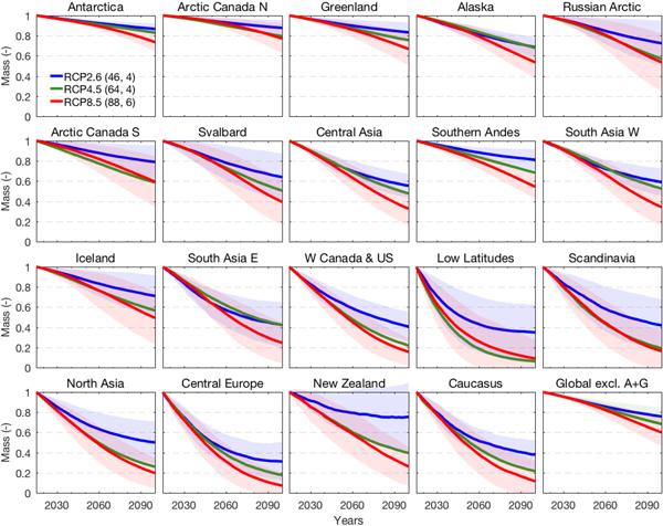
With few exceptions, all six glacier models project glacier mass losses in all regions by the end of the century relative to glacier mass in 2015 for all GCMs and emission scenarios, but losses vary substantially between regions (Fig. 4, Supplementary Figs S1 and S2). Relative volume losses by 2100 (average of all model runs ±1 Std dev.) range from 12 ± 8% (Arctic Canada N) to 69 ± 19% (Central Europe) for RCP2.6, and 23 ± 15% (Arctic Canada N) to 93 ± 10% (Central Europe) for RCP 8.5 (Fig. 5). Only one model's multi-GCM mean shows an increase in glacier mass over the 21st century in one region (New Zealand, RCP2.6, GIE2013, Supplementary Fig. S1). Regions with relatively little ice cover and generally smaller glacier sizes have the most drastic relative mass losses. For example, in Central Europe, Caucasus, Low Latitudes and Scandinavia most glacier model's multi-GCM means project the glaciers to almost completely disappear by the end of the century for the RCP8.5 scenario. In contrast, highly glacierized regions with generally large glaciers tend to have lower projected relative mass losses regardless of the emission scenario (e.g. Arctic Canada North, Antarctic periphery).

Fig. 4. Projected time series of glacier mass 2015–2100 for 19 regions, and globally excluding the Antarctica and Greenland periphery (A + G), based on RCP8.5. Glacier mass is normalized to mass in 2015. Thick lines show multi-GCM means and thin lines mark the results from individual GCMs. Projections for the two Arctic Canada and three High Mountain Asia regions are not available spatially differentiated from SLA2012. Regions are sorted according to initial glacier volume in 2015. Normalized projections for RCP2.6 and RCP4.5 are shown in Supplementary Figs S1 and S2, respectively, and projections in specific units (m w.e. a−1) in Supplementary Figs S3, S4 and S5).
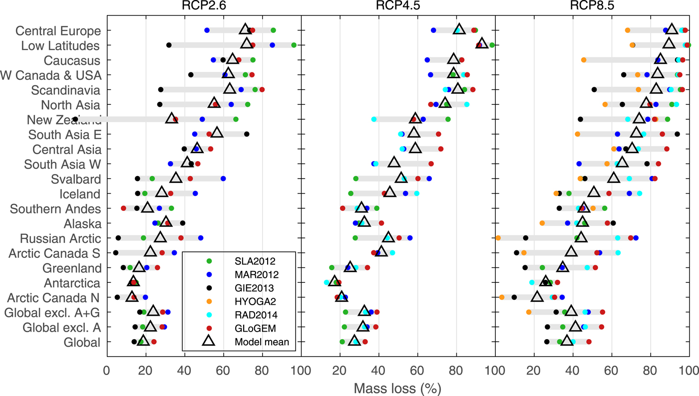
Fig. 5. Projected mass losses by 2100 in percent of the glacier mass in year 2015 for 19 RGI regions from six glacier models using three RCP emission scenarios. Dots mark the multi-GCM means for each glacier model connected by gray bars, and triangles show their arithmetic mean. Regional results are sorted by the glacier models' mean mass loss according to the RCP8.5 scenario. Results are also shown for all regions combined (global), and all regions excluding the Antarctica periphery (A), and excluding the Antarctica and Greenland periphery (A + G). Note that not all glacier models compute all regions or use all three emission scenarios. The data are available in the Supplementary Material.
The spread among projections within individual regions is generally larger than the spread of the global-scale projections (Fig. 4). The spread is particularly large in some Arctic or sub-Arctic regions (e.g. Iceland, Russian Arctic, Arctic Canada South, Svalbard). The largest spread is found in Iceland where individual runs of the six glacier models range from negligible mass losses to complete disappearance. For all emission scenarios, the spread between the model results tends to be comparatively small for MAR2012, RAD2014 and GloGEM, i.e. those models that are structurally relatively similar (Table 1), while results, especially from HYOGA2 and GIE2013, deviate substantially in many regions from most other relative volume evolutions (Figs 4, 5, Supplementary Figs S1 and S2). These two models generally project smaller relative volume changes than the other four models.
Figure 6 illustrates how time series of mass changes by 2100 relative to 2015 vary between the three RCPs. For almost all regions the differences between the three RCPs are negligible or small until the middle of the century but projections increasingly diverge towards the end of the century. As expected the spread of projections for the same RCP also increases throughout the century. In some regions projections based on RCP4.5 are similar to those based on RCP2.6 (Alaska, High Mountain Asia and Antarctic periphery) while in other regions they match more closely those based on RCP8.5 (W Canada & USA, Arctic Canada, Iceland, Russian Arctic, North Asia and Low Latitudes) possibly reflecting differences in regional temperature and precipitation trends. In Arctic Canada S and Low Latitudes modeled relative mass losses for RCP4.5 even slightly exceed those from the more aggressive RCP8.5 scenario which may be an artifact due to the different sets of GCMs and glacier models used for each RCP (see Section 5).

Fig. 6. Projected time series of glacier evolution 2015–2100 for 19 regions, and globally excluding the Antarctica and Greenland periphery (A + G), based on three RCPs. Glacier mass is normalized to mass in 2015. Thick lines show the means of all model projections (all available glacier models and GCMs) based on the same RCP, and the shading marks±1 Std dev. (not shown for RCP4.5 for better readability). Numbers in parentheses refer to number of model runs for each RCP followed by number of glacier models. Regions are sorted according to initial glacier mass in 2015.
Despite generally only modest relative volume losses compared to the other regions, the Antarctic periphery, Alaska, Arctic Canada N, Greenland periphery and the Russian Arctic are the largest regional-scale glacier contributors to sea level for all emission scenarios due to large glacier area (66% of global total (RGI Consortium, 2017); Fig. 7). The SLE contributions of these regions vary among the glacier models' projections, but on average these regions make up 60–67% of the contribution to global SLE by 2100 (average of glacier models' multi-GCM means), depending on the emission scenario. However, for these regions, there is considerable spread among the glacier models, especially for RCP8.5. For example, multi-GCM means for Arctic Canada N vary from ~5 mm SLE (HYOGA2) to 45 mm SLE (RAD2014) by 2100. The sea-level contributions from Low Latitudes, Scandinavia, North Asia, Central Europe, Caucasus and New Zealand combined are negligible (<1% of global) for all RCPs despite generally high relative glacier mass losses, but regional glacier areas are small.
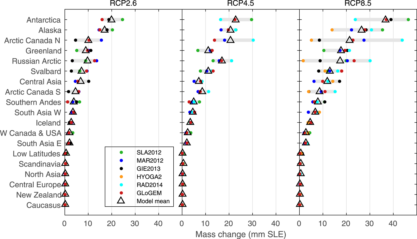
Fig. 7. Projected mass changes 2015–2100 in sea-level equivalent (SLE) for 19 RGI regions from six glacier models using three RCP scenarios. Dots mark the multi-GCM means for each glacier model connected by gray bars, and triangles show their arithmetic mean. Regional results are sorted by the models' mean according to the RCP8.5 scenario. The data are available in the Supplementary Material.
Time series of regional rates of sea-level contribution from glaciers for all regions and RCP8.5 are shown in Figure 8 (see Supplementary Figs S6 and S7 for RCP2.6 and RCP4.5, respectively). All model runs except for SLA2012 (which is not forced by transient meteorological time series) show considerable interannual variations. For all regions and all four emission scenarios, at least one glacier model shows some years with negative SLE rates (especially for the lowest emission scenario), indicating annual glacier mass gains, despite overall regional mass loss trends. In regions with relatively little ice cover (e.g. Caucasus, Central Europe, New Zealand) HYOGA2 shows considerably larger interannual variability with maximum rates an order of magnitude higher than the other glacier models and unrealistic rates of specific mass loss in some years (Supplementary Fig. S5). The causes are unclear but may be related to the implementation of the model, for example, the quantile method used to correct for biases in the GCM data, or the upscaling method used for glaciers <2 km2 (Hirabayashi and others, Reference Hirabayashi, Zang, Watanabe, Koirala and Kanae2013).

Fig. 8. Projected rates of glacier mass loss (mm SLE a−1) 2015–2100 for 19 RGI regions from six glacier models using RCP8.5. Also shown are global mass losses excluding Antarctica and Greenland (A + G). Note that not all glacier models compute all regions or use all emission scenarios. Projected rates for RCP2.6 and RCP4.5 are shown in Supplementary Figs S6 and S7, respectively. Note that the scale varies between regions. Regions are sorted according to initial glacier mass in 2015.
For all emission scenarios, the general temporal patterns of 21st-century rates of SLE varies strongly between the regions, and for some regions also between glacier models (Fig. 8). For RCP8.5, rates generally increase throughout most of the 21st century for regions with large ice cover (e.g. Arctic Canada N, Greenland periphery, Alaska) and where area losses relative to 2015 are small compared to other regions. In contrast regions with small initial ice cover (e.g. Central Europe, Scandinavia) show a steady decrease in rates of SLE consistent with their strongly shrinking mass and area. In some regions of intermediate glacierization (e.g., Central Asia, Iceland, Svalbard), rates first increase as air temperatures rise, and then decrease, despite continued temperature rise, since the glacier extent is progressively reduced.
4.3. Glacier area projections
Global area losses by 2100 relative to 2015 (excluding Antarctic and Greenland periphery) projected by the individual glacier models range from 22 ± 5% to 33 ± 9% (multi-GCM mean ± Std dev.) for the RCP2.6 scenario (three glacier models) and 32 ± 6% to 60 ± 10% for RCP8.5 (five glacier models). Figure 9 shows that regional and global glacier mass loss by 2100 relative to 2015 correlates linearly with corresponding relative area loss for all glacier models and all RCPs. A linear correlation is surprising given the strongly nonlinear relation between volume and area applied in the scaling methods used in most glacier models (Table 1). Possible causes may be related to the size distribution of the global glacier sample and the disappearance of many smaller glaciers by the end of the century but further analyses would be necessary to fully explain this linearity.
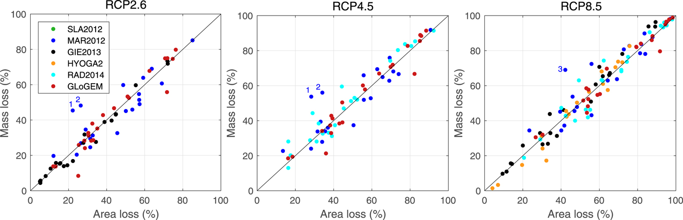
Fig. 9. Modeled regional mass losses versus area losses by 2100 relative to 2015 (%) for three RCP scenarios. Dots refer to multi-GCM means of five glacier models and all modeled RGI regions and the global means. Black line shows the 1:1 line. Area loss data are not available for model SLA2012. Outliers marked by 1, 2 and 3 refer to Iceland, Russian Arctic and Svalbard, respectively. The data are available in the Supplementary Material.
Results from MAR2012 show the largest spread. This is likely caused by their approach to parameterize glacier geometry change, which translates changes in glacier volume to changes in glacier area and length delayed by the glaciers' response times. This implies that if glaciers are losing mass fast compared to their response time, they get thinner first, and lose length and area later.
5. DISCUSSION
Despite consistency in the general pattern of mass loss projected over the 21st century, results indicate substantial spread in projected mass change, especially at the regional scale. The spread indicates that the glacier models have different sensitivities to climate change. We calculate global mass-balance sensitivity S to temperature for all glacier projections according to
 $$S = \displaystyle{{\overline {{\bar{B}}_{2091-2100}-{\bar{B}}_{2015-2024}}} \over {{\bar{T}}_{2091-2100}-{\bar{T}}_{2015-2024}}}$$
where  $\bar{B}$ is the global specific mass balance (mm w.e. a−1) resulting from each GCM scenario, $\bar{T}$ is the corresponding global mean near-surface air temperature of the forcing GCM, and subscripts refer to the averaging years. Sensitivities are plotted against $\bar{T}$ in Figure 10 indicating systematic differences between the glacier models, although the spread is large.
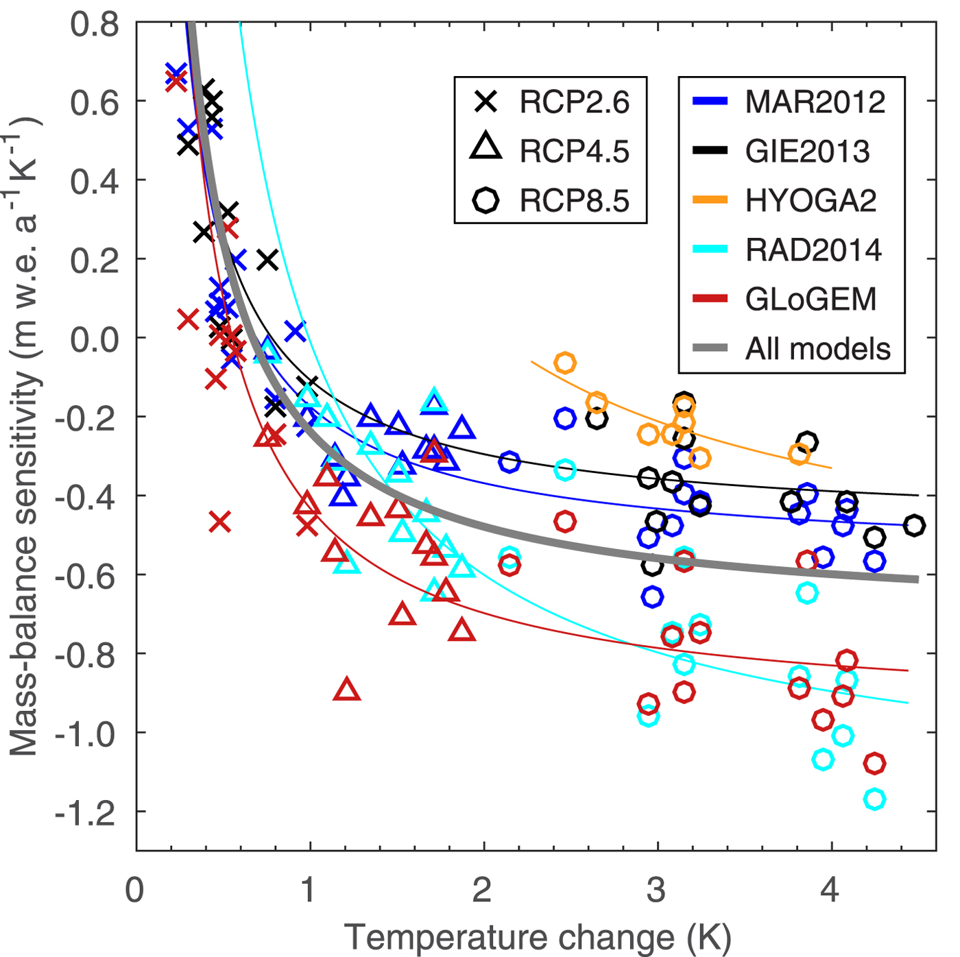
Fig. 10. Global mass-balance sensitivity (i.e. change in the specific global mass-balance rate per 1 K air temperature increase) as a function of changes in global mean near-surface air temperature 2015–2100. Sensitivities are computed from Eqn 1 for all glaciers globally excluding the Antarctic and Greenland periphery. Symbols refer to the three RCP emission scenario and colors mark five glacier models. Sensitivities could not be computed for SLA2012 since glacier area data are not available.
Results also suggest that absolute sensitivities increase as global mean air temperature rises, a pattern that is consistent between the glacier models. A growing disequilibrium between climate and glacier geometry is likely to contribute to this trend. Sensitivities vary from >0.5 m w.e. a−1 K−1 for small temperature increases to <−1 m w.e. a−1 K−1 for temperature increases of ~4 K. Positive sensitivities for global mean temperature increases are counterintuitive but can arise from regional temperature trends deviating from the global mean as well as changes in other meteorological variables affecting the glacier mass balance, in particular precipitation. For a temperature rise of ~1 K (0.8–1.2 K) the mean sensitivity is −0.26 m w.e. a−1 K−1 which is lower than global sensitivities reported in the literature based on modeling or mass-balance observations (−0.39 w.e. a−1 K−1 (Oerlemans, Reference Oerlemans1993); −0.37 w.e. a−1 K−1 (Dyurgerov and Meier, Reference Dyurgerov and Meier2000); −0.68 m w.e. a−1 K−1 (Hock and others, Reference Hock, de Woul, Radić and Dyurgerov2009)).
In addition to differences in sensitivities inherent to each model, the multi-GCM means for the same emission scenario may differ because each glacier model is forced by a different number and ensemble of GCMs with only partial overlap of GCMs (Supplementary Table S1). Temperature and precipitation trends over the investigated time period vary substantially among the GCMs (Fig. 2). Hence, the composition of the GCM ensemble can be expected to affect the projected glacier evolutions.
To address this problem, we compare relative mass losses by 2100 relative to 2015 for the four GCMs (CNRM-CM5, MRI-CGCM3, MIP-ESM-LR, NorESM1-M) forced by RCP8.5 that were used by all six glacier models (Fig. 11). Results indicate a substantial spread among the models for all GCMs with maximum differences in relative mass loss of more than 60% in several regions for at least one of the GCMs (e.g. Caucasus, Svalbard, Arctic Canada South). The largest spread is found in the Russian Arctic (CNRM-CM5), where the six glacier model projections range from <10% to more than 90% mass loss by 2100. Since all models are forced by the same GCM and emission scenarios, these differences result from other factors, such as differences in model physics, calibration procedures, input data and initial ice volume, and downscaling procedures (which in some models are inherently intertwined with the calibration process).
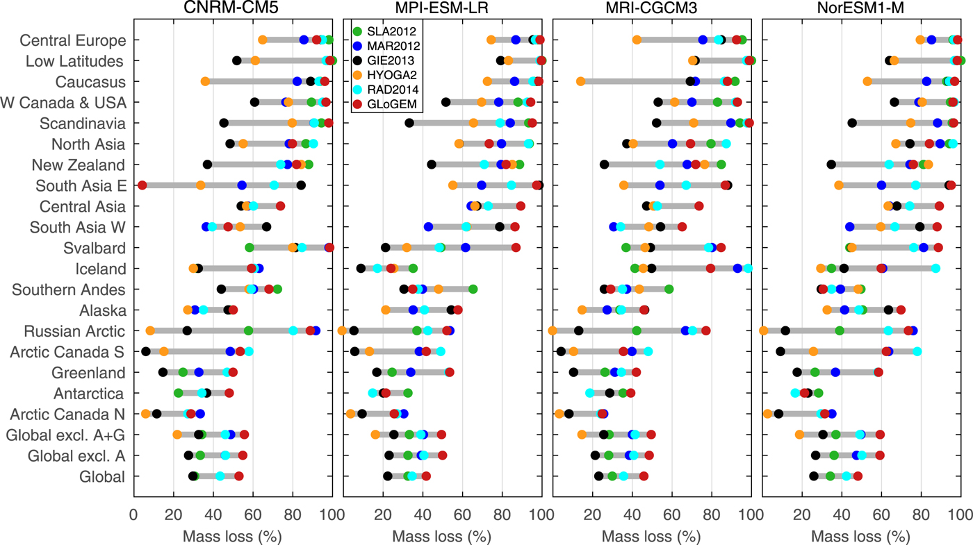
Fig. 11. Projected mass losses by 2100 in percent of the glacier mass in year 2015 for 19 RGI regions and globally excluding Antarctic and Greenland periphery (A + G) based on the four GCMs that were used by all six glaciers models. Results are based on RCP8.5. Dots mark the results for each glacier model connected by gray bars. Regional results are sorted as in Figure 5.
Quantifying the individual contributions of these factors to the model differences is hampered by feedback processes. For example, initial glacier volume varied by almost a factor of two (Figs 3d–f), directly affecting relative mass losses, and also the evolution of cumulative SLE and associated rates, since with less initial volume a region's glacier mass will be depleted earlier, which in turn will provoke further unique mass-balance elevation feedbacks (Bodvarsson, Reference Bodvarsson1955; Huss and others, Reference Huss, Hock, Bauder and Funk2012).
We suspect that the vastly different methods and datasets for calibrating model parameters of the six glacier models are an additional major contributor to differences in the results, especially in light of scarcity of high-resolution data that were available for these studies. Several models were calibrated using regional mass balances spanning multiple years (e.g. GloGEM, HYOGA2). However, modeled balances may match observations with parameter sets that produce small melt and small accumulation rates as well as parameters that lead to high rates of melt and accumulation, but the mass-balance sensitivities will be different thus affecting the projections. Using seasonal balances from individual glaciers allows for separate calibration of melt and accumulation parameters (e.g. RAD2014), or including the model's ability to mimic the temporal variance of observed annual mass balances in the calibration allows one to better constrain the sensitivities (e.g., MAR2012), but uncertainties arise from assigning model parameters to the unmeasured glaciers. All glacier models suffered from scarcity of data for calibration.
6. CONCLUSIONS
Glacier mass projections over the period 2015–2100 from six glacier models each forced by 8–21 GCMs and at least one of four RCP scenarios show substantial global-scale glacier mass losses, especially for the higher emission scenarios. Relative mass losses are generally largest in regions with little ice cover, but due to limited glacier area, their sea-level contribution is small or negligible. However, in these regions, the glacier losses may alter amounts and timing of basin runoff (e.g., Kaser and others, Reference Kaser, Großhauser and Marzeion2010; Huss and Hock, Reference Huss and Hock2018) thus potentially affecting livelihoods further downstream. A few highly glacierized regions account for most of the sea-level contribution although relative mass losses tend to be considerably smaller than for regions with less ice cover. We find large differences between results from the six glacier models for identical RCPs, especially for individual glacier regions, and attribute these to differences in model physics, calibration procedures, downscaling procedures, input data and initial ice volume, in addition to different number and ensembles of GCMs.
In recent years glacier inventory data necessary for model initialization (e.g. area, volume) have been updated and improved (e.g. RGI Consortium, 2017; Farinotti and others, Reference Farinotti2019) allowing future modeling efforts to reduce the uncertainties related to initial conditions. In addition, in particular due to major advances in remote-sensing technologies, many new datasets of glacier mass change with unprecedented coverage and temporal resolution have recently emerged (e.g., Zemp and others, Reference Zemp2015; Brun and others, Reference Brun, Berthier, Wagnon, Kääb and Treichler2017; Braun and others, Reference Braun2019; Zemp and others, Reference Zemp2019). These data provide unique opportunities to better constrain model parameters and also validate global glacier models, thus further reducing the uncertainties in future global and regional-scale glacier projections.
We further recommend standardized experiments for the next-generation global-scale glacier models that prescribe the glacier inventory version, initial glacier volumes and ensemble of GCMs and emission scenarios to guarantee better comparability of results from different glacier models and to evaluate the causes of differences in mass-balance sensitivities. Such standardization will help to guide further improvements in model physics and calibration procedures and is targeted in the next phase of GlacierMIP. Ideally, all models also use the same observational datasets for parameter calibration and validation, and model performance is evaluated with identical statistical criteria to allow direct comparison of the models' ability to reproduce past glacier mass and area changes.
AUTHOR CONTRIBUTIONS
AB, BM, RG, YH, MH and AS submitted their previously published data to GlacierMIP. AB compiled the data in a consistent format and provided initial code to read it. RH designed the study, performed all data analyses and calculations, made all figures except Figure 1, and wrote the paper. AB assisted with coding figures. All authors, in particular MH, commented on the paper.
SUPPLEMENTARY MATERIAL
The supplementary material for this article can be found at https://doi.org/10.1017/jog.2019.22
ACKNOWLEDGEMENTS
GlacierMIP is sponsored by the ‘Climate and Cryosphere’ (CliC) program, and we thank in particular Gwenaelle Hamon, for providing administrative support for GlacierMIP. RH was supported by NASA grants NNX17AB27 G and 80NSSC17K0566 and NSF award # 1543432, and AB by NASA grant NNX11AO23G. AS was supported by the NWO-Netherlands Polar Programme and a CSIRO Office of the Chief Executive Postdoctoral Fellowship, RG by the ice2sea project, funded by the European Commission's 7th Framework Programme through grant # 226375, and BM by the German Federal Ministry of Education and Research (grant 01LS1602A). Matvey Debolskiy provided invaluable help with coding the figures. Orie Sasaki made Figure 1. Haireti Alifu calculated the global mean GCM time series. David Rounce checked the language.


 Open access