

Introduction
The grounding zone is the transition between the grounded ice sheet and the floating ice shelf, and is one of the most sensitive parts of the ice-sheet system (Reference SchoofSchoof, 2007). It is an important boundary for ice-sheet modelling, as this is where the shear stress at the bed is removed, and ice accelerates, spreads and thins. Grounding zones are also regions of high basal melting, as the temperature of sea water in the ice-shelf cavity is above the pressure-melting point. This effect increases with ice draft (Reference Jacobs, Hellmer, Doake, Jenkins and FrolichJacobs and others, 1992; Reference Shepherd, Wingham and RignotShepherd and others, 2004; Reference Pritchard, Ligtenberg, Fricker, Vaughan, Van den Broeke and PadmanPritchard and others, 2012). As ocean properties are modified by climate change, melting in grounding zones is likely to increase, with the potential to greatly impact ice-flow dynamics (Reference Joughin, Alley and HollandJoughin and others, 2012). To properly estimate the effects of rising ocean temperatures on the mass balance of outlet glaciers and future stability of ice shelves, it is vital to know basal melt rates in this sensitive area, and to be able to precisely measure the mass input to the ice shelves from outlet glaciers. Both of these calculations require measurements of ice-thickness cross sections in the grounding zone.
Traditional satellite-based methods for measuring the thickness of floating ice assume that ice is close to hydrostatic equilibrium (and therefore make a simple calculation of thickness from freeboard and ice density; e.g. Reference StearnsStearns, 2011) but uncertainties may be in the range 80– 120 m in the grounding zone (Reference RignotRignot and others, 2008). A more accurate ice-thickness estimate can be made further downstream, where the ice is fully floating; however, this excludes the grounding-zone region which is typically several kilometres wide, depending on ice thickness and ice properties (Reference Fricker, Coleman, Padman, Scambos, Bohlander and BruntFricker and others, 2009; Reference BindschadlerBindschadler and others, 2011). This not only underestimates the ice thickness but potentially overlooks significant basal melting in the grounding zone. Conversely, applying the hydrostatic equilibrium assumption at the landward limit of tidal flexure results in an overestimate of the ice thickness, as the ice is at least partially grounded and supported by the land (Reference VaughanVaughan, 1995); downstream, however, the ice may be partly depressed below hydrostatic equilibrium (Reference Fricker and PadmanFricker and Padman, 2006) and thickness consequently underestimated. Because of both the limitations in deriving the ice-thickness cross sections in the grounding zone and the complications in observing horizontal ice flow by interferometry, tidal-flexure zones are sometimes excluded from the remote-sensing analysis of melt rates (Reference Neckel, Drews, Rack and SteinhageNeckel and others, 2012). Alternatively, ice thickness can be measured using ground-penetrating radar (GPR), but the spatial coverage is then confined to the tracks measured and, in many areas, there is limited potential for multiple repeat measurements to identify thickness change.
In this study, we demonstrate that an inverse formulation of plate-bending equations, based on simple elastic assumptions, can be used to solve for ice thickness using vertical deflection information. We use differential synthetic aperture radar (SAR) interferograms to estimate vertical displacement, which provide unprecedented accuracy and form the input for the model. We conduct a thorough sensitivity analysis of the model configuration and glaciological parameters in one and two dimensions. We then create satellite interferograms for Beardmore Glacier, an outlet glacier in the Transantarctic Mountains, and validate the numerical results against ground measurements of thickness which we collected in 2010. GPS measurements in this grounding zone allow us to validate vertical displacement in the interferograms and assess the applicability of an elastic-beam model by looking at temporal variation in our ‘effective’ Young’s modulus.
The Ice Shelf as an Elastic Beam
Tidal displacement of ice consists of an instantaneous elastic deformation accompanied by a time-dependent visco-plastic deformation (Reference HughesHughes, 1977). The vertical displacement of an elastic beam of ice due to ocean tides has been described by Reference HoldsworthHoldsworth (1969) and Reference VaughanVaughan (1995), and the theory has been expanded to cover two-dimensional (2-D) elastic plates (Reference Schmeltz, Rignot and MacAyealSchmeltz and others, 2002). Although GPS measurements in Greenland have shown that a viscoelastic deformation model more fully describes the vertical deflection in this region, reproducing both phase and amplitudes of tidal deflections (Reference Reeh, Mayer, Olesen, Christensen and ThomsenReeh and others, 2000, Reference Reeh, Lintz Christensen, Mayer and Olesen2003), elastic models are shown to widely replicate amplitudes of flexure in interferometric SAR (InSAR) observations when a lower ‘effective’ Young’s modulus is used (Reference RignotRignot, 1996; Reference Schmeltz, Rignot and MacAyealSchmeltz and others, 2002; Reference Jenkins, Corr, Nicholls, Stewart and DoakeJenkins and others, 2006; Reference Sykes, Murray and LuckmanSykes and others, 2009).
Ice subject to stresses for short durations exhibits elastic or viscoelastic behaviour, depending on the shear modulus of the ice, which, in turn, depends on ice temperature, density and degree of damage (Reference Schulson and DuvalSchulson and Duval, 2009). Reference GudmundssonGudmundsson (2007) shows that for periods of applied stress over a few seconds, ice behaves elastically with an elastic response equal to the instantaneous Young’s modulus of ice, E, similar to that measured in laboratory experiments (e.g. Reference Petrenko and WhitworthPetrenko and Whitworth, 1999). However, while a value of E = 9: 33 GPa is measured for isotropic polycrystal-line ice in laboratory studies (Reference Petrenko and WhitworthPetrenko and Whitworth, 1999), E = 0: 88 ± 0: 35 GPa is shown to fit better with field data collected on a number of glaciers in both Antarctica and Greenland (Reference VaughanVaughan, 1995). This difference can be attributed to the partially viscous deformation, the importance of which depends on the timescale under consideration. Over periods of a few minutes, ice behaves as a viscous material, while at periods of hours to days, ice behaves almost purely elastically, with a lower effective Young’s modulus producing a delayed elastic response (fig. A1 of Reference GudmundssonGudmundsson, 2007). Reference GudmundssonGudmundsson (2007) expects an almost purely elastic response on Rutford Ice Stream for cold ice subject to tidal oscillations of between 1 hour and 50 days, with the importance of viscous flow increasing rapidly with temperature. The maximum duration of applied stress for which ice remains in this elastic state depends on the effective viscosity, which is related to ice temperature and shear stress. The applicability of a purely elastic model will therefore vary from location to location.
The elastic deformation of a one dimensional (1-D) beam of variable flexural rigidity is given by the well-known fourth-order Euler–Bernoulli equation (Reference HoldsworthHoldsworth, 1969):
where ▽ is the gradient operator (∂/∂x), w is the vertical displacement, f is the applied load and D is the flexural rigidity given by
where E is the Young’s modulus,ν is Poisson’s ratio and h is ice thickness.
The flexural rigidity is exponentially dependent on the thickness. Published values of Poisson’s ratio do not vary significantly from ν = 0: 3, which is the value adopted throughout this study, but an order of magnitude in the range of values has been reported for E (Reference VaughanVaughan, 1995; Reference Schmeltz, Rignot and MacAyealSchmeltz and others, 2002). With the method described here it is not possible to distinguish between the separate glaciological parameters which determine the flexural rigidity of ice, so it is assumed that ν and E do not vary spatially across the domain and the observed variation in flexural rigidity depends only on ice thickness. The consequent potential error in thickness due to variation in the glaciological parameters is discussed in parallel with the sensitivity analysis of modelling and regularization parameters.
Equation (1) can be split into a system of two second-order differential equations (e.g. Reference Schmeltz, Rignot and MacAyealSchmeltz and others, 2002):
where M is the applied moment. For a beam supported by ocean water and affected by tidal forces, f = ρ w g (T – w) where T is the magnitude of the tide and ρ w is the density of ocean water.
The inverse formulation to estimate flexural rigidity (i.e. thickness assuming a constant value for E and) is ill-posed, meaning that small errors in initial data (the flexure measurements) can propagate into much larger errors and mesh-dependent oscillations about the correct value in the results (Reference Lucchinetti and StüssiLucchinetti and Stüssi, 2002). This issue can be overcome by regularization, which in this case involves penalizing solutions with steep gradients or change in gradient of thickness, minimizing either h or2 h. Additional constraints (e.g. the maximum allowed rate of change of thickness) can be imposed in order to expedite the convergence on a numerical solution.
Model Implementation
Calculating ice flexure for glaciers is essentially a three-dimensional (3-D) problem with stress and strain estimated in x, y and z, but, as we are solving for thickness it requires only a 2-D geometry. The elastic beam theory is first described for a 1-D case, with model configuration tested on synthetic profiles representing potential thickness distributions across an Antarctic grounding zone. The 1-D problem is essentially a cantilever beam, fixed at the grounding-line end, w( 0) = w 1 (0) = 0, and freely floating at the ice-shelf end, w″ (x max) = 0; w ″(xmax) = 0, with applied vertical load depending on vertical displacement, w. The load is due to the tidal force, which in the inverse model is known, a priori, from the interferogram. A clamped boundary with zero rotation is used to represent the grounded ice boundary (e.g. Reference VaughanVaughan,1995; Reference Reeh, Lintz Christensen, Mayer and OlesenReeh and others, 2003). Grounding-line migration is also disregarded. This treatment of the grounding line contrasts with the simply supported boundary approach tested elsewhere (Reference Sayag and WorsterSayag and Worster, 2011; Reference Walker, Parizek, Alley, Anandakrishnan, Riverman and ChristiansonWalker and others, 2013) but avoids the need for modeling stresses upstream of the grounding line and simplifies analysis of the inverse model for ice resting on a solid foundation. The 2-D version of the model relies on the same constituent equations for beam bending, applied to a 2-D domain, with lateral boundary conditions, w ” (y 0) = 0; w(y max) = 0.
The solution of the forward model for an elastic beam agrees well with the analytical solution (Reference HoldsworthHoldsworth, 1969; Reference Schmeltz, Rignot and MacAyealSchmeltz and others, 2002). Here we test the inverse approach using two synthetic beams of exponentially and linearly decaying thickness, as well as beams with additional Gaussian undulations in the centre. The model is initially run forward to predict vertical movement from known thickness and then a white noise Gaussian error is added to simulate uncertainty associated with the input interfero-grams caused by low phase coherence and resolution. The inverse model is then used to recalculate thickness and estimate the propagation of error associated with the optimization routine. A comparison of input and output thickness for these two scenarios shows the deviation resulting from the instability of the inverse approach (Fig. 1).

Fig. 1. Comparison of (a) input flexure with modelled flexure and (b) input thickness and modelled thickness for a 1-D exponentially decaying thickness profile. Input thickness is used to create flexure data, random noise in a normal Gaussian distribution is added to simulate the error in an interferogram and then the inverse model uses the flexure information to reproduce ice thickness. The error in modelled thickness introduced by this inversion is shown in (b).
As the inverse problem described here is ill-posed, there exist a number of unique solutions to the thickness profile which satisfy the observed flexure profile. The greater the number of nodes in the finite-element mesh, the more closely the problem approximates the ill-posed continuous problem and becomes more ill-conditioned (Reference Lesnic, Elliott and InghamLesnic and others, 1999). For conversion into a well-posed problem with an optimal solution, the objective function can be modified by adding a ‘penalty function’, and the thickness estimated using a least-squares optimization routine. The weighted sum of the data error and the penalty function is known as the Tikhonov functional (Reference Tikhonov and ArseninTikhonov and Arsenin, 1977):
Where λ is the regularization parameter and г is the regularization operator. In this case the second-derivative operator, ▽2, is used as the regularization operator. This minimizes the curvature of the thickness profile and skews the result towards a profile with a uniform change in thickness. Model runs were also conducted using the first-derivative operator, г = ▽ (i.e. minimizing the change in thickness and therefore skewing the results towards a constant value), but this was less effective at approximating the correct solution for undulating thickness profiles, potentially present in ice-sheet grounding zones (e.g. Reference DutrieuxDutrieux and others, 2013). Regularization reduces large fluctuations in thickness and as λ is increased, the solution becomes further biased towards a uniform thickness and ‘real’ oscillations in thickness are lost. The selection of a suitable value for λ is vital to sufficiently constrain the minimization near the floating margin without unnecessarily biasing the solution and smoothing out genuine thickness deviations closer to the grounded ice boundary.
All modelling of ice flexure was conducted with commercial finite-element software, COMSOL Multi-physics, using the SNOPT (Sparse Nonlinear Optimizer) algorithms for model optimization. This uses a forward-gradient method to return the spatial values of thickness which minimize the Tikhonov functional. The optimization routine iterates the forward model and compares the least-squares difference between modelled vertical displacement and the vertical displacement observed in the interferogram. Additional constraints are imposed on the minimization, including inequality bounds on values of thickness, and limits on maximum thickness gradient. These conditions act to stabilize the solution more rapidly and ensure that unrealistic thickness fluctuations cannot occur. Sensitivity of the output to each of these parameters is discussed in more detail in the following section.
Results from Sensitivity Analysis
We initially analysed a 1-D synthetic profile, in order to determine the viability of the inverse method and to identify the optimum parameters for the model across a straight grounding line given expected noise in the interferograms. After selection of model parameters, additional sensitivity tests were conducted in 2-D for a sinuous grounding line, in order to assess the potential range in final thickness results caused by the choice of parameterization at embayments and land protrusions. The sensitivity of the inverse approach is tested with regard to: noise in the interferogram; the Tikhonov regularization parameter, λ; glaciological parameters associated with the flexural rigidity (Young’s modulus, Poisson’s ratio, density of ice); model convergence parameters and runtime; shape and discretization of the mesh; and the size of the domain. The sensitivity is quantified by looking at the magnitude of variability in thickness output in relation to the magnitude of changes to the input variables. The percentage change in ice thickness at the grounding line and mean ice thickness in the grounding zone are calculated, as well as maximum deviation from the expected thickness within the grounding zone. The results for these tests on an exponentially decaying ice-thickness profile are given in Table 1, and examples of output profiles in Figures 2–4. Model convergence parameters had little effect on the final solution, except to modify the time taken for convergence, and with an appropriate choice of regularization parameter fining of the mesh also produced no improvement in output thickness. For this exponentially decaying thickness profile, increasing the size of the domain to greater than approximately double the grounding-zone width (in this case 12 km) does not affect the thickness results within the grounding zone. Reducing the size of the domain below 12 km, however, causes a divergence from the synthesized thickness close to the downstream margin of the grounding zone, where some residual flexure is observed and therefore does not match the freely floating condition specified in the model at this boundary, w ”(x max) = 0; w″ (x max) = 0. A reduction in the domain to 10 km caused a divergence of >25% from the expected thickness in the region between 7 and 10 km from the grounding line. The thickness results for the upstream 7 km were not affected. Reference Sayag and WorsterSayag and Worster (2011) suggest that for a domain greater than a threshold distance related to a set buoyancy-bending length scale, further increases in the domain size should have a negligible effect on the flexure pattern. A value of 12 km provides approximately 6–7 times their calculated length scale for ice of constant thickness with the synthesized stiffness used here.

Fig. 2. Sensitivity of the inverse 1-D model to additional noise added to a simulated interferogram. All runs are on an exponentially decaying thickness profile with λ = 1 × 10²².

Fig. 3. Sensitivity of the inverse 1-D model to the value of Young’s modulus, E. All runs are on an exponentially decaying thickness profile with λ = 1 × 10–22 and noise = 2%.

Fig. 4. Sensitivity of the inverse 1-D model to variation in . All runs are on an exponentially decaying thickness profile with constant noise at 2%.
Table 1 Sensitivity of 1-D model runs to changes in glaciological and regularization parameters using an exponentially decaying synthesized thickness profile. Model optimization was continued until a tolerance threshold was reached on the optimality criteria, or a maximum limit on the number of iterations was reached. Unless otherwise stated, parameters used are E = 1 GPa, ν = 0.3, noise = 2% and λ = 1 × 10–22

With ideal input parameters, the inverse model converges rapidly on a solution within 1% of the measured thickness close to the grounding line. Downstream of the point of maximum vertical displacement (~ 6 km in Fig. 1) the gradient of the flexure profile observed in the interferogram is reduced and deviation from the measured thickness becomes more pronounced. As the distance from the grounding line increases, changes in ice thickness become less important in determining the flexure pattern and small errors in the flexure can more greatly affect the resulting thickness. This is particularly highlighted by the 10% noise profile in Figure 2.
Glaciological parameters
Variations in Young’s modulus within the range observed for outlet glaciers (Reference VaughanVaughan, 1995) can have a significant effect on the estimated thickness at the grounding line and throughout the flexure zone (Fig. 3). The relative thickness remains representative when an incorrect value of E is used, but absolute thickness is incorrectly estimated with a constant percentage offset from the measured thickness, proportional to the error in the estimate of E. Where field measurements of thickness are not available to correct this offset to obtain a more appropriate value for E in the grounding zone (i.e. modifying E by matching modelled and observed thickness data), a best approximation can be made close to the downstream margin of the grounding zone using the hydrostatic equilibrium assumption. Adjusting the density of ice, ρ ice, and Poisson’s ratio, ν, within a realistic range for outlet glaciers had little effect on the thickness (Table 1). The effect of a firn layer on flexural rigidity is accounted for in the chosen value of Young’s modulus.
The regularization parameter, λ
The choice of λ depends on the difference between the observed flexure from the interferogram and the flexure predicted by the Euler–Bernoulli equations from a perfect thickness profile. The two main components that determine this parameter are therefore background noise within the interferogram (i.e. the interferogram not matching the actual ice flexure) and the assumptions within the model (e.g. the small but nonzero error in flexure caused by neglecting viscous effects, shear deformation and rotational inertia).
Sensitivity to interferogram noise and phase bias was analysed to assess the suitability of using interferograms with areas of low coherence as input to the model. White noise in a Gaussian distribution was added to the synthesized flexure profile before being used as input to the inverse model to simulate the interferogram. For reference, the high-frequency noise in the unsmoothed TerraSAR-X interferograms is ~ 1 cm, or ~ 2% of the observed tide in interferograms from Beardmore Glacier. Results are shown in Figure 4 and Table 1.
Thickness undulations
The 1-D model performs well in the grounding zone where ice thickness decays linearly or exponentially downstream. However, the Euler–Bernoulli equations do not account for shear deformation within the ice and cannot resolve small-scale undulations. Furthermore, the high dependence of the whole ice flexure profile on the ice thickness closest to the grounding line makes resolving small-scale undulations further downstream of this point more difficult. The regularization method penalizes these undulations in favour of a more smoothed profile and the strength of the regularization parameter is therefore also important in determining the width and amplitude of undulations which may be resolved. The model has been tested with a number of synthetic thickness bumps added to the profile at different locations, to estimate the potential of the model to capture these small-scale spatial variations in thickness. Gaussian pulses of different width and amplitude are introduced at three locations within the grounding zone: 1, 3 and 5 km, respectively, downstream of the grounding line. The results of this testing indicate that for E = 1 GPa, bumps greater than two to three ice thicknesses in width close to the grounding line can still be identified, but when they occur close to the freely floating margin their influence on the ice flexure decreases and they are not resolved in the inverse model.
Two-dimensional effects
Sensitivities for an elastic beam, as discussed above, are equivalent to the sensitivities for a perfectly straight grounding line in 2-D with uniform ice thickness and ice properties in the perpendicular direction. Grounding zones are rarely straight lines, however, and although the 1-D beam approach can work well in many glaciological situations, the numerical model can also be applied to thin elastic plates with irregular plan view geometry. Sensitivity tests in 2-D generally reproduce the results demonstrated in 1-D (Table 1) where the grounding zone is linear or concave downstream, although sensitivity appears to be greater at convex grounding lines. Sensitivity to the regularization parameter is shown in Figure 5 for a sinusoidal grounding zone with exponentially varying thickness. Figure 5f further demonstrates how the regularization parameter affects the thickness derived at the grounding line, with an increase in λ leading to smoothing of ice thickness with reduced accuracy, but a decrease in λ leading to unrealistic oscillations about the mean.

Fig. 5. Sensitivity to the regularization parameter in 2-D for a sinusoidal grounding line. (a) Mesh and model domain. (b) Input thickness. (c) Modelled thickness deviation from the input with initial conditions of h = 500 and λ = 1 × 10²¹. (d) As (c) with λ = 1 × 10²². (e) As (c) with λ = 1 × 10²³. (f) Thickness along the curved section of the grounding line (A–B), shown in (a).
In the forward model, concave embayments have a much greater effect on the observed flexure than convex protrusions (e.g. Reference Rabus and LangRabus and Lang, 2002). In contrast, the inverse model shows greater sensitivity to convex protrusions. The technique described here requires a higher value of the regularization parameter to smooth out fluctuations at these locations (Fig. 5). A possible explanation for this is that there is a reduced area of contact with the fixed boundary near the region for which a solution is sought. Overall, while the quality of the inverse model can be analysed using a synthetic flexure pattern with a simple grounding-line geometry, differences between a forward elastic-plate model and actual ice behaviour have also been observed at real grounding zones, particularly at embayments and inlets (e.g. Reference Schmeltz, Rignot and MacAyealSchmeltz and others, 2002). This cannot be tested using a synthesized flexure profile and is validated using field data.
Validation of Modelled Thickness for Beardmore Glacier
Beardmore Glacier (83.5° S, 172° E) drains a catchment of ~ 90 000 km2 from East Antarctica into the Ross Ice Shelf (Fig. 6) and is ~ 25 km wide at the grounding line. A notable feature of the grounding-zone region is a line of equidistant rifts propagating downstream from the grounding line, interpreted by Reference Collins and SwithinbankCollins and Swithinbank (1968) to be caused by ice passing over a high point on the bed, with thicker ice either side. This is supported by radio-echo sounding (RES) measurements from December 1967 (personal communication from C. Swithinbank, 2010). We acquired GPR data in the grounding zone during December 2010 using a 25 MHz pulseEKKO system (Fig. 7c). A domain for Beardmore Glacier is traced from differential interferograms based on the extent of the flexure zone. Expansion of the domain into the ice shelf has negligible effect on the thickness results, but identification and correct location of the fixed boundary at the grounding line are vital to produce reliable thickness maps. The grounding zone is identified here from the upstream limit of flexure observed in the interferogram (Fig. 8a and b) (e.g. Reference Rignot, Mouginot and ScheuchlRignot and others, 2011). The relative interferometric phase due to ice flexure is unwrapped using the average vertical displacement over the grounded ice to fix the displacement map to 0 (Fig. 8c).

Fig. 6. Location of Beardmore Glacier, East Antarctica.

Fig. 7. (a) A map of Beardmore Glacier grounding zone showing locations of ice-thickness cross sections, 2012 TerraSAR-X interferometric (dashed black) and ASAID (Antarctic Surface Accumulation and Ice Discharge; solid black) grounding lines (Reference BindschadlerBindschadler and others, 2011). (b–d) The thickness from our flexure model is compared to (b) thickness derived from ICESat surface elevations (orbit 1353 – L3B; A–B); (c) a GPR radar profile acquired in 2010 (C–D); and (d) thickness derived from an Advanced Spaceborne Thermal Emission and Reflection Radiometer (ASTER) digital elevation model (DEM), and airborne RES acquired in 1967 (E–F).
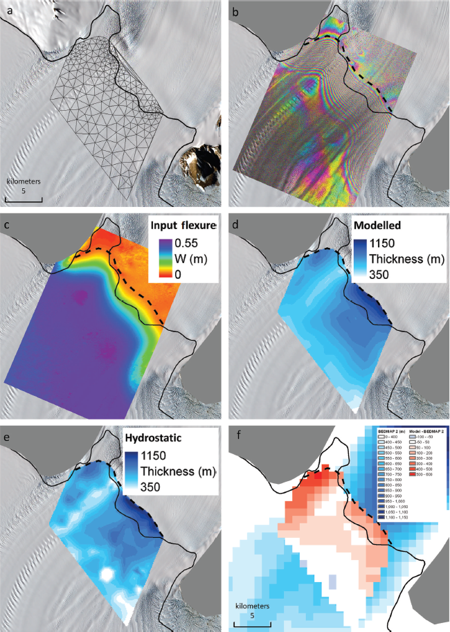
Fig. 8. (a) Beardmore grounding zone with model domain and mesh. (b) TerraSAR-X differential interferogram showing tidal-flexure fringes. (c) Differential vertical displacement derived from an unwrapped interferogram. (d) Inverse modelled ice thickness (λ = 1 × 10- 20). (e) Thickness assuming hydrostatic equilibrium from ASTER DEM. (f) Difference between Bedmap2 thickness data and model results.
Vertical displacement input data
As input for the model, we acquired vertical displacement information using InSAR. InSAR uses the phase difference in two or more SAR images acquired at different times and slightly different locations to accurately identify surface displacement (Reference Goldstein, Engelhardt, Kamb and FrolichGoldstein and others, 1993). Interference between the images allows centimetre-scale changes in slant range, either related to topography or surface deformation, to be identified. Differential InSAR (DInSAR) allows removal of the contribution of topography, leaving only information about the change in displacement between images. In the grounding zone, any change in displacement over satellite repeat periods is related strongly to vertical movement of the ice under the influence of ocean tides (Reference Marsh, Rack, Floricioiu, Golledge and LawsonMarsh and others, 2013), and the difference in movement between grounded and floating areas has been widely used to map grounding lines around Antarctica (Reference GrayGray and others, 2002; Reference Brunt, Fricker, Padman, Scambos and O’NeelBrunt and others, 2010; Reference Rignot, Mouginot and ScheuchlRignot and others, 2011).
We use InSAR data from the TerraSAR-X mission (Reference Breit, Fritz, Balss, Lachaise, Niedermeier and VonavkaBreit and others, 2010) in stripmap mode, which provides 9.65 GHz, 3.3 m azimuth resolution and ~ 2.5 m slant-range resolution data on an 11 day repeat cycle. Reference Rabus and LangRabus and Lang (2002) noted that care must be taken when looking at quadruple tide difference at four individual tides (i.e.t 1 − t 2) − (t 3 − t 4Þ) and that large errors can be made in locating the grounding line where this difference is less than ~ 10% of the dynamic variation in tide. Here TerraSAR-X triples are acquired at periods of significant tidal variation and differenced, (t 1 − t 2) – (t 2 − t 3), to maximize the signal-to-noise ratio of the flexure data (Table 2). Although two other triples were acquired, they failed to produce good-quality, coherent displacement maps for this glacier. As the differential baseline for the TerraSAR-X pairs is small, the topography is neglected in calculating the tidal flexure.
Table 2 TerraSAR-X acquisitions with radar incidence angle at the scene centre for the Beardmore grounding zone, with corresponding values of modelled ocean tide from CATS2008a_opt (Reference Padman, Fricker, Coleman, Howard and ErofeevaPadman and others, 2002). All acquisitions are in stripmap mode from beam 014, track 039 in descending orbit

Validity of the elastic-plate model
Flowline modelling shows that the basal ice temperature at the grounding line of Beardmore Glacier is around − 5°, with average surface temperatures of − 25°C (N.R. Golledge and others, unpublished information). Calculation of the complex modulus of ice suggests that the amplitude of deformation caused by diurnal tidal oscillations should be well described by an elastic model at this location, despite requiring a modified (and lower) value for the Young’s modulus to account for the deformation due to primary creep over shorter timescales. GPS data obtained in the grounding zone of Beardmore Glacier also support a time-invariant value for the effective Young’s modulus at this location (GPS-3 of Reference Marsh, Rack, Floricioiu, Golledge and LawsonMarsh and others, 2013). A time series of vertical deflection from this study lags behind a regional tide model (CATS2008a_opt) by 22 min. However, assuming a fixed grounding-line position and thickness derived from GPR, the deflections observed in the GPS data produce a constant value for ‘effective’ E at the centre of the glacier of 1: 5 ± 0: 5 GPa.
Initial thickness estimate
Thickness can only be estimated from the flexure profile up to 5–10 km from the grounding line, where there is still differential vertical displacement. Ice that is further away than this (i.e. where the ice moves vertically in synchronicity with the tides) should, however, be in hydrostatic equilibrium and its thickness can be estimated from the freeboard. An initial estimate for the equivalent ice thickness is inferred using the principle of hydrostatic equilibrium. Where ice is in hydrostatic equilibrium its thickness is given by
where h eq is the equivalent thickness, h f is the freeboard, F c is the firn correction andw andi are the densities of water and ice, respectively. Grounding-line position and the geometry of the model domain is obtained from the extent of TerraSAR-X imagery and the interferograms used to map flexure. Grounding-line migration is limited at this location due to steep topography. A triangular mesh is used which decreases in size towards the grounding line, with spacing between nodes of 1 km on the ice shelf and ~ 500 m in sensitive areas close to the grounding line (Fig. 8a). The model is not sensitive to the initial estimate for thickness near the grounding line, as a difference of <1% is observed when comparing a model run with constant initial thickness and initial thickness based on the freeboard estimate. The sensitivity to initial conditions is higher close to the floating margin of the domain, increasing to almost complete dependence on initial thickness outside of the flexure zone, due to the progressively lower importance of ice thickness in this region in determining flexure.
We produced ice surface elevations for Beardmore Glacier from an Advanced Spaceborne Thermal Emission and Reflection Radiometer (ASTER) stereographic satellite image pair at 30 m resolution. The ASTER digital elevation model (DEM) was linearly adjusted to fit Ice, Cloud and land Elevation Satellite (ICESat) elevations. Photogrammetry produces high-quality DEMs in grounding zones of steep outlet glaciers and, although there is probably no systematic offset due to the applied ICESat correction, this DEM still has a standard deviation of 16 m at the grounding line in comparison to ‘best-available’ elevation measurements from the Antarctic Surface Accumulation and Ice Discharge (ASAID) project (Reference BindschadlerBindschadler and others, 2011). Modelled firn density varies between 13.5 and 14.5 m in this area, and a constant firn correction of 14 m is applied to the elevation data to obtain an initial thickness estimate (Van den Reference Van den BroekeBroeke, 2008). All data are linearly interpolated onto the mesh. A ground-based longitudinal thickness transect across Beard-more Glacier at a central point is used here as field validation and to obtain a reliable estimate of the Young’s modulus, although close agreement with ice thickness from ICESat-based hydrostatic equilibrium calculations close to the hydrostatic line suggests that a satellite-only technique could also be used at this location. Output for the model is shown in Figure 8d with a direct comparison of GPR and RES thicknesses, hydrostatic-equilibrium-derived thickness and model thickness at linear transects in Figure 7.
Discussion
Sensitivity analysis shows that changes in model domain extent, discretization and tolerance on convergence have a small effect on the final thickness distribution. Initial conditions are also unimportant with regard to data quality close to the grounding line, although a reasonable initial approximation of ice thickness and Young’s modulus reduces the time taken for the model to converge to a solution which agrees with GPR measurements. In the 1-D case, the inverse model reproduces steady variation in ice thickness well, with models of both linearly and exponentially decaying thickness profiles downstream of the grounding line agreeing to within 1–2% with actual thickness. The 1-D analysis shows that the inverse approach may be a useful tool for calculating ice thickness in the grounding zone where the grounding line is relatively straight. The quality of thickness results in this simple case depends on the amount of noise in the initial input data (the interferogram) as well as the value of the Tikhonov regularization parameter. The Tikhonov parameter must be tuned to reduce the effect of the noise within the interferogram but not bias the thickness close to the grounding line by excessive smoothing. At Beardmore Glacier, for low interferogram noise levels (where phase unwrapping is possible) and with a tidal amplitude of 50 cm, a regularization parameter of 1 × 10⁻²⁰ allows for a stable thickness map which agrees with radar measurements to within 50 m root-mean-square error. The optimum value of this parameter depends on the rate of spatial thickness variation and model domain characteristics and may therefore be site-specific. The synthetic 2-D case (Fig. 5) suggests that a value of ~ 1 × 10–21 yields best results across the grounding zone. Methods of calculating the optimum value for this parameter without additional information are discussed elsewhere (e.g. Reference Lucchinetti and StüssiLucchinetti and Stüssi, 2002) but are beyond the scope of this study and require further work.
In 2-D, the pattern of flexure also depends on grounding-zone shape, with complex grounding zones affecting the observed flexure pattern. As demonstrated by sensitivity testing on synthetic flexure profiles, where the elastic-theory describes the flexure pattern in the forward model, the inverse model reproduces thickness well. It requires further investigation using real observed flexure patterns at other locations to determine the wider applicability of this technique, particularly at convex grounding zones, where the observed flexure is probably not as well described by the simple model, and for warmer glaciers, where viscoelastic effects may have a greater influence on the observed amplitude of vertical displacement.
Where glacier thickness varies smoothly across the grounding zone, the thickness produced from flexure is shown to agree to within 10% with the thickness used to produce those flexure data. In contrast, synthetic flexure profiles produced from profiles with an introduced bump in thickness highlight the current limitations of this method in complex or undulating grounding zones. As the flexure profile already incorporates a smoothing based on the local rigidity, small undulations do not affect the interferogram and cannot be estimated using the inverse model. In particular the model fails to resolve asperities less than two to three ice thicknesses in width. More significant features, however, such as the relatively thin-ice region of rifting around 5 km wide on Beardmore Glacier are still resolved, and ice-thickness changes can be identified. In the cross section shown in Figure 7b the modelled thickness deviates by up to 150 m from the thickness predicted by an assumption of hydrostatic equilibrium based on ICESat data from 2009. This deviation is similar to that expected if the ice is supported above hydrostatic equilibrium at the grounding line and depressed below hydrostatic equilibrium a few kilometres downstream. The model agrees reasonably well with radar data, although it tends to smooth out large features (Fig. 7c and d). Differences in the long profile are likely due to GPR errors induced by side reflectors if the pattern seen in Figure 7d is a typical cross section. Large percentage differences between modelled and hydrostatic thickness on the ice shelf in Figure 8e are due to the exaggerated sensitivity of thickness derived from the DEM to small artefacts in the surface elevation. Agreement with Bedmap2 thickness (Reference FretwellFretwell and others, 2013) is also within the range of expected error at this location (300 m), except to the east of the rifts where the modelled thickness is much greater but Bedmap2 disagrees with GPR measurements (Fig. 8f).
The sensitivity analysis highlights the importance of a good value of ‘effective’ E to ascertain the correct thickness at the grounding line. Although the ‘effective’ E may vary within a small range for Antarctic outlet glacier grounding zones, a 50% error in E can introduce an ~ 18% error in grounding-line thickness. E can be inferred by adjusting the mean modelled thickness at the downstream boundary of the grounding zone (here 10 km) to the value expected from hydrostatic equilibrium. We find a value of 1.4 GPa suitable for the Beardmore Glacier grounding zone for this particular time period, which is at the upper limit of values found by Reference VaughanVaughan (1995) in grounding zones around Antarctica, but within the range observed by Reference Schmeltz, Rignot and MacAyealSchmeltz and others (2002) using a similar approach. Comparison of the tidal-flexure pattern from the forward model driven by Circum-Antarctic Tidal Simulation (CATS) tidal data and our GPS measurements in the grounding zone (Reference Marsh, Rack, Floricioiu, Golledge and LawsonMarsh and others, 2013) suggests that the value of the effective E does not vary over time at this location.
Conclusion
We have shown that information about the way in which ice responds to ocean tides can be used to estimate ice thickness in the Antarctic grounding zone. Centimetre-scale variations in ice movement are obtained from satellite data by creating differential interferograms. This can be converted into thickness estimates using an inverse formulation of the elastic-plate equations. A regularization parameter constrains the minimization routine. This is a novel technique which provides a method of measuring ice thickness in this sensitive area without the need for surface or airborne GPR measurements. Modelled ice-thickness results on Beard-more Glacier agree with GPR measurements that we collected in the field. The accuracy of the ice thickness produced depends on the value taken for the effective Young’s modulus, but a good approximation of the Young’s modulus can be made at point locations where ice thickness is known, either through a hydrostatic equilibrium calculation outside the grounding zone or from GPR measurements. The satellite-based technique could also, therefore, be used to spatially extend existing thickness data generated from sparse, linear ice-thickness transects.
In order to obtain high-accuracy vertical displacement information we have created high-resolution, low-noise interferograms using TerraSAR-X data. Under normal circumstances, interferograms which are able to be unwrapped have sufficiently low noise for this technique, and can easily be further smoothed with only a minor impact on the resulting ice thickness. As undulations less than a few ice thicknesses do not strongly influence the flexure pattern, they cannot be resolved by this method. Nonetheless, the improvement in ice thickness at the grounding line compared to the standard hydrostatic equilibrium thickness method is expected to be 10–15%, even where the quality of the available freeboard data for the hydrostatic method is very high.
The model used here is sensitive to noise in the input interferogram and particularly relies on accurate location of the landward limit of the grounding zone, but it is possible to obtain this location to a sufficient degree of accuracy in interferograms where phase coherence is high. The double difference tidal range of 0.5 m observed here is relatively small compared to the mean tidal range around the perimeter of Antarctica (Reference Padman, Fricker, Coleman, Howard and ErofeevaPadman and others, 2002). Larger differences in tidal displacement increase the ability to model the thickness by reducing both background noise in the inter-ferograms and the contribution of viscoelastic effects to the flexure pattern.
We validated our ice-thickness retrievals with in situ data at Beardmore Glacier, and obtained good agreement with centre-line thicknesses of 900 m from our GPR data and 800 m from Bedmap2 (Reference FretwellFretwell and others, 2013). As the pattern of the tidal flexure depends on the geometry of the grounding line, it remains to be investigated how well the method performs for more complex grounding-line configurations or fjord-like embayments. The application of a purely elastic model to warmer glaciers experiencing more viscous deformation also requires further investigation. We expect improved results compared to the freeboard-thickness method, where the interferometric grounding-line position is well defined and the elastic model accurately describes the pattern of tidal flexure.
Acknowledgements
We thank Charles Swithinbank for information pertaining to the 1967 Beardmore Glacier RES data, and Antarctic New Zealand Event K001B-Ice and Dean Arthur for field and logistical support. This research was funded, in part, by the Ministry of Business, Innovation and Employment, through research contract CO5X1001 to GNS Science. TerraSAR-X data were provided by DLR from science proposal HYD1421. ASTER data were provided through the Global Land Ice Measurements from Space (GLIMS) project. Comments from Helen Amanda Fricker and three anonymous reviewers led to substantial revisions and improvement of the paper.


