


A Notable contribution to the structure of the ice shelf at the Little America V I.G.Y. station, Antarctica, was made in November and December 1958, when a 14.6 cm. wide hole was drilled to a depth of 255 m. or to within about 5 m. of the bottom. This was done by a U.S. Army-S.I.P.R.E. drill team as part of the U.S.-I.G.Y. Antarctic Program. w cm. cores and temperatures were obtained to the bottom of the hole. Details of the drill operation and measurement of temperature are being published.Reference Ragle, Hansen, Gow and Patenaude 1 In the present paper an attempt will be made to interpret the Little America vertical temperature profile in terms of real heat and latent heat of fusion supplied to the ice shelf by the underlying ocean, using as supplementary or verifying data, observations of ice thickness and motion. Also, a steady-state solution associated with vertical motions will be discussed. Comparisons will be made with the ice shelves near Maudheim and the Ellsworth I.G.Y. station.
The Observed Temperature Profile
In Fig. 1 are plotted the observed temperatures of the Little America hole (lat. 78° 11′ S., long. 162° 10′ W.; 44 m. a.s.l.). The temperatures are believed to be accurate to ±0.1° C. The snow temperature of −22.3° C. at 10 m. depth was measured 25 m. away from the deep hole by H. Neuberg. The −22° C. snow temperature at 12.2 m. depth was observed below the floor of the snow laboratory a few meters from the deep hole. Four points, designated by squares, represent air temperatures at designated depths in the hole where the thermometer had been allowed to come to equilibrium for 12 or more hours. The remaining points, designated by circles, are temperatures observed by a thermometer in contact with the bottom of the hole and presumably embedded in a thin layer of ice “dust” remaining after the drilling bit was withdrawn. Both the air and snow temperatures agree quite well in the region of overlap between 60 and 110 m. However, the two air temperatures at 12.2 and 43 m. appear to be slightly too high, perhaps caused by the steel casing extending 41 m. into the hole.

Fig. 1. Little America observed temperatures in ice shelf designated by points. Computed temperatures based on heating with and without melting
The temperature increases with depth, more and more rapidly with increasing depth. The bottom temperature of −4.4° C. was observed at 250 m.; the drilling was continued to 255 m. where the ice cores still showed no signs of salinity. Later, sea-water seeped into the hole and froze. Re-drilling was attempted but no temperatures at greater depth were obtained. The extrapolation of a smooth curve going through the observed points intersects −1.8° C., the freezing point of salt water of 33 parts per thousand salinity, at 259 m. depth,Footnote * which is the upper limit of ice thickness that N. A. Ostenso detected by seismic shooting near the drill hole in November 1958.
Computed Temperature Profiles with No Melting
A curve drawn through the observed temperatures in Fig. 1 appears to depart from the near-straight line quasi-equilibrium temperature profile which would result if an ice shelf, 259 m. thick, initially isothermal at −22.3° C., had remained over a −1.8° C. ocean for 400 yr. without melting or vertical motions. Other profiles are drawn for residence times of 200, 100 and 50 yr., with no melting. Footnote † Curve “a”, drawn for 100 yr. residence time over the ocean, agrees so well with the observed temperatures (mean deviation of only 0.85° C.), that it is tempting to state that the problem is solved, that Little America V is on an ice shelf that has been over the ocean for 100 yr., that in this interval the ice shelf has moved northward from the nearest land, Roosevelt Island, whose closest point to Little America V is 60 km. (see Fig. 5, p. 635). This would mean a movement of 0.60 km./yr. or 1.65 m./day, a value in quite reasonable agreement with an earlier estimate by Gould.Reference Gould 2 In essence this analysis would mean that the Little America V ice shelf is just an ice “run-off” from Roosevelt Island, whose ice cover is believed to be an ice cap formed from local accumulation on the island and not part of the original Ross Ice Shelf which moved over the island in its northward motion.Reference Zumberge 3
However, the assumption of no melt during the century of residence over the ocean is a worrisome matter which requires further consideration. (The possibility of significant accretion of ice from below because of sea-water freezing is eliminated because of lack of saline ice within 5 m. of the bottom of the ice.) Our doubts are further increased by the fact that the ice at the northern tip of Roosevelt Island is about 400 m. thick,Reference Crary 4 greater than that found at Little America V, 259 m. If this is the same ice layer moving northward one would have to account for the vertical loss of 141 m. of old ice plus 20 m. of accumulated ice during the century the ice took to move 60 km. to the north. The effect of melting at the bottom must be considered; no appreciable melting and run-off occur at the top surface in summer, since the average December–January surface air temperature at Little America V is −6.1° C. Also there is a possibility that sinking motions caused by horizontal divergence of the ice shelf Reference Robin 5 could account for some of the thinning of Roosevelt Island ice in its motion northward; this effect will be discussed later.
Computed Temperature Profile with Bottom Melting—I
In Fig. 1 we add a new curve “b” for 100 yr. of heating and bottom melting. This new curve is computed under the assumption that the energy is conducted to the bottom of the ice from an ocean whose temperature stays “just above” the −1.8° C. freezing point of 33 parts per thousand saline sea-water and that this energy is partitioned equally between heating the ice shelf and melting a portion of it.Footnote * In 100 yr. 9.3 m. of ice are melted and the temperature profile becomes the curve designated by curve “b” in Fig. 1. This curve agrees somewhat better with the observed temperatures (see Table I) but both computed curves suffer from the same defect of large positive departures from the observed temperatures in the lower half of the ice shelf. In fact, in the lowest 30 m., the observed temperatures fall almost exactly on the 50 yr. no melt curve.
Table I. Little America V Hole, Observed Temperatures and Computed Minus Observed Deviations (°C.)

The melting of 9.3 m. of ice in 100 yr., or an average of 9.3 cm./yr. would be only 6 per cent of the observed thinning if the ice had moved from Roosevelt Island, and less than half of the annual water accumulation at Little America V. Let us now see what the result would be without arbitrarily assuming equipartition of energy into heating and melting.
Computed Temperature Profile with Bottom Melting-II
The rate of melting and heating of an ice shelf lying on an ocean will be influenced by the rate at which energy is transported to the ice bottom by the warmer ocean. The ice-water interface is assumed to remain always at the freezing point of sea-water of salinity 33 parts per thousand, or −1.8° C. If the water far below the ice bottom (or more precisely at a depth corresponding to the bottom of the ice before melting began; see Appendix B) is kept at a temperature, ΔT, above the freezing point, then the heat transport to the ice bottom will be conducted primarily by eddies created by turbulent motions in the ocean currents under the ice.
One way of measuring the coefficient of eddy conductivity in the oceans is by observing the variations of the seasonal amplitude and lag of temperatures at various depths. In the open ocean this can vary from 16.4. to 2.1 g. cm.−1 sec.−1 at 0 to 50 m. in the Bay of Biscay and from 78 to 23 g. cm.−1 sec.−1 in the Kuroshio Current.Reference Sverdrup 6 The strong current of the Kuroshio Current would lead to greater eddying motions than in the Bay of Biscay and the latter would probably also have stronger eddying motions than the water under the Ross Ice Shelf. Hence a value of eddy conductivity equal to 1 g. cm.−1 sec.−1 was initially assumed for the calculations outlined in Appendix B.
In Fig. 2 is drawn curve “c” computed under the assumption that ice, initially isothermal at −22.3° C., is in contact for 100 yr. with water whose deep temperature is −1.7° C., or 0.1° C. above the freezing point, and which has an eddy conductivity of 1 g. cm.−1 sec.−1. During these 100 yr. 24.4 m. of ice would be melted from the bottom. Curve “c” is in fairly good agreement with the observed temperatures below 175 m. but has quite large negative deviations above.

Fig. 2. Little America observed temperatures in ice shelf designated by points. Computed temperatures based on heating with melting
In Fig. 2, curve “d” is plotted under the assumption that ice, initially isothermal at −22.3° C., is in contact for 200 yr. with water whose temperature below the ice bottom is −0.8° C. and which has an eddy conductivity of 1 g. cm.−1 sec.−1. During this 200 yr. period 120.1 m. of ice would be melted from the bottom. The temperature profile is given by curve “d” which agrees better with the observed temperatures than any of the previous computed curves.
Of all four curves constructed thus far, curve “d” fits the observed points best with curves “b” and “c” next and curve “a” last.
It should be emphasized that the four curves discussed herein were computed under the assumption that there exists in the ice shelf no vertical motions. Because of the constant thickness of the Maudheim Is-shelf despite an annual accumulation of 40 cm. water equivalent, Robin has stressed this process and has shown that there exists a steady-state temperature profile which is not linear.Reference Robin 5
Let the origin of the x-axis be located in the surface of an ice shelf of thickness H, with x positive downward.
Assume that the shelf thickness, H, remains constant by an annual accumulation, W 0, which is off-set by a sinking of the ice layers at a speed of w 0 and a melting rate at the bottom of w 0 cm. yr.−1. If the ice layers move with no change of temperature, then
represents the local change of temperature.
If conduction of heat occurs, then (1) becomes
where
-
κ = K/ρc = 1.15×10⁻² c.g.s. units is the thermal diffusivity of ice,
-
K = 5.3×10⁻³ is its thermal conductivity,
-
ρ = 0.92 is its density,
-
c = 0.5 is its specific heat.
Equation (2) has been solved by BenfieldReference Benfield 7 in finding the temperature of an accumulating snow field subjected to a periodic surface temperature.
For a steady-state
which can be easily solved if κ and w 0 w are independent of x. The solution is
where a = −w 0/κ and C 1 and C 2 are constants.
Although not written explicitly in his 1955 paper, this is Robin’s solution for the special case of bottom melting equal to surface accumulation. Introducing the boundary conditions:
Taking T0 = −22.3° C. and T H = −1.8° C., two curves are plotted in Fig. 3: curve “e” for w 0 = 50 cm. yr.−1 and curve “f” for w 0 = 20 cm. yr.−1. The respective equations are:

Fig. 3. Little America observed and computed temperatures for steady-state sinking, with constant shelf thickness
As may be seen in Fig. 3, the observed temperatures of the Little America hole fit curve “e” quite well but depart widely from curve “f”. As shown by Table I, the average deviation of the points from curve “e” is 0.18° C. with the maximum deviation of only 0.5° C.
At Little America V, the average annual accumulation is about 20 cm. ice equivalent. Suppose that the ice shelf thickness remains constant despite this annual accumulation; then the ice layers in the shelf must sink at a rate of 20 cm. per annum (except for the surface layer where greater motions occur because of compaction of the snow and firn). But the resulting steady-state temperature profile, curve “f”, fits the observed temperatures very poorly, while curve “e” drawn-for a 50 cm. per annum sinking, fits the observed points almost perfectly. As is well known the accumulation apparently can vary greatly in short distances. For example, at Little America I, located 60 km. south-west of Little America V, 20 m. of two 21.5 m. high radio towers erected in January 1929, were covered by snow in 30 yr.Footnote * Extrapolating Schytt’s formula II relating water accumulation to depthReference Schytt 8 gives an accumulation of about 38 cm. water equivalent or 41 cm. ice equivalent. But even this higher, probably nonrepresentative, accumulation rate is less than the 50 cm. of ice accumulation which yields the curve of best fit. If the good agreement of curve “e” is not merely a coincidence but has physical significance, this means that the sinking rate is 2.5 to 1.2 times larger than the annual accumulation, i.e. the shelf is not maintaining constant thickness but is thinning at a rate of 30 to 9 cm. per annum. This can be brought about by a melting rate larger than the annual accumulation or by a horizontal spreading of the ice shelf or both, but each of these processes would violate two of the basic assumptions underlying the above calculations, namely, constant shelf thickness and constant sinking rate of ice through the shelf.
It is important to note that there exists a fundamental difference in assumption between the two models of best fit, “d” and “e”, considered here. For model “d” the ice is assumed to have originated in isothermal state over land and moved without vertical motion over the ocean 200 yr. ago, during which time it lost by melting 120 m. of ice and did not attain a state of thermal equilibrium. For model “e” no earlier land history of the ice need be assumed: a steady-state temperature profile exists which agrees remarkably with the observed temperatures provided the sinking rate of the ice layers is 50 cm. per annum, or about 2.5 times the annual accumulation. Because of the difficulty in devising a reasonable physical interpretation of the results of model “e” (despite its nearly perfect agreement with observations) attention will be directed to the results of model “d”.
Energy and Oceanographic Considerations
The great depth of water (300 to 600 m.) beneath the shelf ice at Little America VReference Poulter 9 would permit ample means for water currents to transport heat to the ice bottom. According to PoulterReference Poulter 9 “A current of one to three knots enters Okuma Bay and moves in a south-westerly direction, partly along and partly under the ice at Kainan Bay”. Assume that this current is in contact with an average of 100 km. of ice as it passes under the ice shelf from Okuma Bay to Kainan Bay (see Fig. 5). Let us now compute how much energy this current would have to transport in 200 yr. to heat to the melting point and melt 120.1 m. of ice along a strip 1 cm. wide and 200 km. long and at the same time heat the remaining ice to the temperatures observed in the Little America hole. The assumptions made are that the ice is initially isothermal at −22.3° C. and that the Little America ice heating and melting represent typical conditions in that portion of the ice shelf affected by the ocean current.

We shall assume that as the water emerges from under the ice its temperature is at the freezing point. If ΔT is the initial deviation of the water temperature above its freezing point as the water first comes in contact with the ice bottom, and ΔH is the thickness of the water layer from which energy is abstracted to heat and melt the ice, then in 200 yr. the energy transport by an ocean current of width 1 cm. and speed V cm. sec.−1, is VΔTΔH × 109 cal. This must therefore equal the energy given up to a 1 cm. wide strip of ice along the 100 km. current trajectory, 1055·3×1010 cal.
Thus ΔTΔH = 1.67V −1 × 10².
Some pairs of values of ΔH and ΔT which satisfy this equation for various values of V are shown in Table II.
Table II Initial Temperature, ΔT (above the Freezing Point), and Thickness, ΔH, of the Water Layer Transporting Heat to the Bottom of the Ice Shelf, for Various Current Speeds, V

For example, if 50 m. is the thickness of the water layer below the ice which is the principal source of heat for melting and warming the ice above, then its initial temperature departure from the freezing point of sea-water need only be 0.027° C. for a 0.25 knot current and 0.007° C. for a 1 knot current.
Let us compare the values shown in Table II with observed ocean temperatures in the vicinity of the ice shelf.
Oceanographic soundings made a few kilometers north of the ice shelf at. Little America 10 , 11 revealed temperatures and other data shown in Table III.
Table III Oceanographic Soundings near Little America V (Lat. 78° 11′ S., long. 162° 10′ W.)

The values below the horizontal line correspond to depths below the bottom of the ice shelf at Little America V. The water temperatures at these depths are quite close, within a few tenths of the temperature at which sea-water of the observed salinity and pressure begins to freeze, as shown by the figures in the column headed Tf .Reference Thompson 12
It thus appears unlikely that the temperature of the sea-water under the ice shelf at Little America V can depart from the freezing point of that sea-water by as much as the 1° C. which was assumed in computing the curve of second-best fit, “d”, even if allowance is made for possibly lower salinity and hence higher freezing point. On the other hand curve “c”, which was computed on the assumption of a 0.1° C. deviation from the freezing point, is only the curve of third-best fit (see Table I). Another variable, of course, is the intensity of the mixing processes which transport heat to the bottom of the ice. A low value 1 g. cm.−1 sec.−1 was assumed in computing curves “c” and “d”. The values may be higher, and it is therefore of some interest to compute melting rates as a function of eddy conductivity, A, and temperature above the freezing point of sea-water, ΔT. This can be done by means of equation (14) given in Appendix B. The results for an ice shelf, initially isothermal at 20.5° C. below the freezing point of sea-water, are shown in Fig. 4 for both 100 and 200 yr. melting (the latter melting rates are the numbers in parentheses).

Fig. 4. 100 and 200 yr. curves of constant ice melt as function of ocean eddy conductivity, A, and temperature of seawater above its freezing point, ΔT
As expected the curves of equal melt are hyperbolic in appearance. It is seen that at a given ΔT, the melting rate increases slower than A. Thus for ΔT = 0.2 °C. and A = 2, the 100 yr. melt is 50 m.; for A = 16, it is 150 m. An inspection of Fig. 4 reveals that for a given ΔT the melting rate is approximately proportional to √A.
Returning to the problem of the ice shelf melt it is seen from Fig. 4 that one can achieve compatibility of the second-best fit curve “d” and its 120 m. of melt with a ΔT = 0.1° C instead of 1° C., by increasing the eddy conductivity, A, from 1 to about 10. (As explained in Appendix B, the temperature distribution in the ice and water will remain the same so long as one selects pairs of values, ΔT and A, from the same curve of constant melt.) Since data on ΔT and A under the Ross Ice Shelf are not available,Footnote * it does not appear possible to arrive at an unambiguous estimate of the time of duration over water and melting rate of the ice shelf at Little America V. Nevertheless, it appears worth while to carry out an exercise using the results of the computation which led to second-best fit curve “d”, and 120 m. of bottom melting in 200 yr., to see if this result is compatible with observations of the speed and direction of motion of the ice shelf near Little America.
Observed Motions of the Ice Shelf near Little America V
In trying to obtain motions of the Ross Ice Shelf in the neighbourhood of Little America V, use has been made of old and new positions of certain ice shelf features such as Framheim (Amundsen’s 1911–12 camp), Kainan Bay, the site of Little America I and the site of Little America III (Fig. 5).

Fig. 5. Eastern portion of Ross Ice Shelf. Large numerals refer to ice thickness in meters at Little America V and northern tip of Roosevelt Island
The data are summarized in Table IV.
Table IV Motions of Ross Ice Shelf near Little America

There is surprisingly good agreement in the absolute motions of the ice shelf taken at various places 60 km. apart. Although each station has a component of motion westward, there are differences in direction. Taking the average of the two values near Kainan Bay, Little America V appears to have moved north-north-west or north-west at 390 m./yr.Footnote * The direction of motion appears to be reasonable if it is interpreted to be along a vector resultant of nearby Roosevelt Island ice cap moving northward and the inland ice of the more distant Marie Byrd Land moving westward towards Roosevelt Island whence it is deflected north-westward or north-north-westward.
Assuming that the motion of 390 m./yr. obtained over the past 200 yr., which is the period of time Little America V ice is presumed to have been in contact with the ocean, we shall try to find its position in 1758. This would be somewhere on an arc of 78 km. radius with Little America V as the center as shown in Fig. 5.
Suppose the ice is moving to the north-north-west, then 200 yr. ago it would have been at the intersection X (Fig. 5) of the 78 km. arc and the north-eastern coast of Roosevelt Island where the present ice thickness is presumably near 400 m.; this could have been the thickness 200 yr. ago.Footnote * If this were so, then 400–259 = 141 m. +40 m. of water equivalent of accumulated snow, or a total of 181 m., would have had to be lost during the 200 yr. journey of the ice to Little America V where the present ice thickness is 259 m. If all this loss of vertical thickness of 181 m. were caused by melting then by interpolation between the 200 yr. (141.4 m.) and (212 m.) curves in Fig. 4, it is seen that this melting could occur with fairly large values of ΔT, compared to those shown in Table III, or with fairly large values of A, compared to the range shown at the bottom of Fig. 4 —neither of which are likely possibilities.
It thus appears that the thinning of the ice shelf as it moves 78 km. from a presumed point X (Fig. 5) to Little America V could not have all been caused by melting from below and that a horizontal spreading of the ice probably plays an important rôle. Since the channel between Marie Byrd Land and Roosevelt Island widens appreciably north of lat. 79° S. (see Fig. 5), this should encourage horizontal spreading. A lateral spreading of the ice by only 16 per cent, in moving from point X to Little America with uniform speed seaward throughout, could account for the thinning from 440 m. of ice at point X (440 = 400 observed + 40 accumulated in 200 yr.) to 379 m. at LAS V (379 = 259 observed + 120 melted). If the speed of the ice seaward increases near the edge of the ice as observed at MaudheimReference Swithinbanle 24 this would also contribute to the thinning of the ice. Of course, the nearer to the sea the more rapid should also be the melting but, as stated above, it would hardly seem possible to explain by melting alone the loss of 181 m. of ice in the presumed 200 yr. of motion from point X to Little America.
The Maudheim Is-Shelf
The availability of temperatures to a depth of 100 m. in the Maudheim Is-shelfReference Schytt 23 permits another case to be examined under conditions different from those of Little America. At Maudheim (lat. 71° 03′ S., long. 10° 56′ W.; 38 m. a.s.l.), the average annual temperature in the top 7 m. of the snow is −17.4° C. instead of −22.3° C. at Little America, the accumulation is close to 40 cm. of water instead of 20 cm. and the shelf thickness is close to 200 m. instead of 259 m. Although the temperatures were measured only to a depth of 100 m., Schytt extrapolated the profile to the sea-water freezing point at the bottom of the ice shelf, which in 1954 he estimated was 185 m. thick.
In Fig. 6 are plotted Schytt’s observed and extrapolated temperatures for the Maudheim Is-shelf. The writer is indebted to Dr. Schytt for furnishing him in advance of publication the numerical values of the observed temperatures, a smoothed curve of which was published in 1954; the extrapolated values were scaled from Schytt’s extension of this curve.Reference Schytt 23 In the following computations the writer used a bottom temperature of −1.8° C., a surface temperature of −17.4° C. and a thickness of 185 m.Footnote †
Three curves are drawn in Fig. 6. The first, curve “a”, is copied from curve (2) of Robin’s Fig. 4 Reference Robin 5 which was drawn on the assumption of bottom melting equal to accumulation in a steady-state model, where the downward velocity of the ice is equal to the annual accumulation and thus the bottom melt rate. Although Robin gives no figure for the ice accumulation value he used in deriving his curve, presumably he took the Maudheim value of 40 cm. yr.−1. This curve departs widely from the observed and extrapolated temperatures.

Fig. 6. Maudheim observed and computed temperatures. Curves “a” and “b” are for steady-state accumulation (sinking) with constant shelf thickness. Curve “c” is for 75 yr. of heating and melting
In Fig. 6 is another curve, “b”, based on the same steady-state model, but using a 109 cm. yr.−1 ice accumulation; this curve fits the observed and extrapolated temperatures quite well. Curve “c” is a non-steady-state solution resulting from the residence for 75 yr. of an ice sheet, initially isothermal at −17.4° C., over an ocean whose deep water temperature under the ice shelf is taken as −0.8° C. and whose eddy conductivity coefficient, A, equals unity. In 75 yr. 75 m. of ice are melted. Curves for 50 yr. (61.1 m. melt) and for 100 yr. (86.5 m. melt), not shown here, depart more widely from the observed temperature than the 75 yr. curve.
Here again, as in the case of Little America, the curve of best-fit is a steady-state model wherein the sinking speed of the ice, 109 cm. yr.−1, is more than double the annual accumulation, 40 cm. yr.−1.
Again, taking into account the assumptions underlying this particular steady-state model, a physical interpretation is difficult. Therefore, once again, we pursue the consequences of the non-steady-state heating and melting model whose 75 yr. curve, “c”, is associated with 75 m. of melted ice. As in the case of the Little America hole, let us back-track the Maudheim hole to where it might have been 75 yr. before 1950.
SwithinbankReference Swithinbanle 24 has estimated the average movement of the Maudheim Is-shelf across the 36 km. width of its discharge channel to be 280 m./yr. In 75 yr., if the speed of motion remained the same, the ice would have been somewhere on an arc of 21 km. radius from Maudheim. The only direction where ice 21 km. from Maudheim is on land instead of ocean is due east, on the coast of Hill A (see Fig. 2, SwithinbankReference Swithinbanle 24 ). If the Maudheim ice had been originally at this spot and had the same thickness there as now it would have been somewhere between 309 and 420 m. thick; these are the respective thicknesses of the two seismic stations straddling the hypothetical point: the first, Station 40, is on the ice shelf and the second, Station 175, is on Hill A.Reference Robin and de 25 If we take an average value, then the thickness of the ice now at Maudheim could have been 365 m. 75 yr. ago. Thus the decrease from 395 (365 m. initially plus 30 m. accumulation in 75 yr.) to 275 m. (200 m. thick now plus 75 m. melt) equals 120 m., which would have to be accounted for by horizontal spreading and vertical shrinking. A horizontal spreading of 43 per cent in the 75 yr. of motion could account for the observed thinning. Swithinbank’s largest area increase in 6 months, 0.176 per cent, was measured for a small triangular area directly east of Maudheim. In 75 yr. this would equal 30 per cent, too small to account for the observed thinning. If the initial ice thickness had been that of the closest observed shelf thickness, 309 m. at Station 40, located 3.7 km. south-west of the hypothetical point, the divergence in 75 yr. need only have been 23 per cent, in fair agreement with Swithinbank’s measurement cited above.
This “exercise” is, of course, interesting but not very conclusive, since it is based on the results of one particular theoretical model and an assumed direction of motion from the nearest grounded ice area (Hill A). From geographical considerations Swithinbank estimated the direction of motion of the Maudheim Is-shelf to be slightly west of north as compared to the due west direction assumed in the above computations.
Because of an apparent discontinuity at 70 m. in the vertical profile of ice crystal area in the Maudheim hole, Schytt speculated that this represented a change from local (shelf) accumulation to the original inland ice.Reference Schytt 8 Since it would take 140 yr. to lay down 70 m. of ice, Schytt believed it took 140 yr. tor the ice to travel from the 650 m. high ridge 45 km. to the south-east of Maudheim, or an average rate of movement of 320 (±80) m. per annum to the north-west. This compares with Swithinbank’s speed of 280 m. per annum in a direction slightly west of north.Reference Swithinbanle 24
According to Fig. 6, Schytt’s estimate of 140 yr. for time of passage of the Maudheim Is-shelf over the ocean would yield temperatures too high in the layer 50 to 100 m. depth; the observed temperatures are colder than the 100 yr. heating curve and of course would be even colder than the 140 yr. curve. But it should be pointed out that for shallow profiles such as Maudheim’s, where most of the temperature measurements are made in ice laid down by accumulation in transit, it is difficult to analyse the thermal history of the entire thickness of the ice shelf. For example, if the inland ice had initially a temperature several degrees lower than the −17.4° C. assumed here, which seems likely, then those temperatures near the bottom of the Maudheim hole are not necessarily incompatible with a 140 yr. residence time over the ocean (see Fig. 9).
The Ice Shelf at the Ellsworth I.G.Y. Station
At the Ellsworth I.G.Y. station (lat. 77° 43′ S., long. 41° 08′ W.; 41 m. a.s.l.) a deep pit was dug to a depth of 31.3 m., and a to cm. hole was drilled in the pit floor to a depth of 56.91 m.Reference Augenbaugh, Neuberg and Walker 26 The pit and hole were located in a north-south oriented trough in the ice shelf 150 m. east of the station and 3.5 m. below the station elevation. Temperatures in the pit were obtained by inserting a thermohm 3 m. into the pit wall at each depth; temperatures in the drill hole were obtained by placing a thermohm at the bottom of the drill hole at the end of each day’s drilling (Table V). The depth at 0.0 m. is the average annual air temperature as measured in the meteorological shelter at the camp site.
The temperatures are plotted in Fig. 7 and show decreasing temperatures from the surface, −23.1 ° C. to −26.7° C. at 43.91 m., a minimum of −26.74° C. at 54.74 m. and finally what appears to be a slight increase to −26.72° C. at 56.91 m., the bottom of the hole. This decreasing temperature with depth at Ellsworth station differs from Little America and Maudheim, where the temperatures increase slowly with depth in the top 57 m. (see Figs. 1 and 6).

Fig. 7. Ellsworth observed and computed temperatures, heating and melting
It would appear that that portion of Filchner Ice Shelf near Ellsworth station differs significantly in thermal history from the ice shelves at Little America and Maudheim. It is tempting to consider that the Ellsworth ice is being heated from above by a warmer atmospheric environment (including accumulation) as well as from below by the warm ocean under the ice shelf which is 232 m. thick and is floating on an ocean 792 m. deep.Reference Thiel 27
Table V Ellsworth Station Deep Pit Temperatures, 1957Reference Augenbaugh, Neuberg and Walker 26

Let us assume a model having these properties: an ice shelf, initially isothermal at −26.74° C., the minimum temperature in the Ellsworth hole, moves from land and floats on an ocean, whose deep temperature is −0.8° C., or 1° C. above the freezing point of sea-water. Using the theory outlined in Appendix B we construct two temperature profiles: “a”, for 50 yr. residence time, during which 58.8 m. of ice are melted, and “b”, for 100 yr. residence time, during which 83.1 m. of ice are melted (Fig. 7). In both cases the eddy conductivity of the ocean beneath the ice shelf was assumed to be A = 1 g. cm.−1 sec.−1 and the effect of sinking of ice was neglected.
In comparing the observed temperatures with the theoretical curves it is seen that curve “b”, the 100 yr. curve, is slightly warmer than the observed points from 57 to 47 m., but that these latter points fall on the 50 yr. curve which, indeed, is isothermal from about 90 m. to the surface.
In attempting to base an estimate of age on the observed points it is critical to know whether the observed temperatures below 41 m. are truly isothermal or decrease to a slight minimum and begin to increase. Since we are dealing with temperatures in the second decimal place we cannot say with certainty whether additional points would follow the 50 yr. curve or perhaps a 75 yr. (72 m. melt) curve. We shall assume the latter curve to be the correct one and attempt to follow through the consequences.
The nearest (ice-covered) land areas from Ellsworth station are Coats Land, 122 km. to the east, and a large island the same distance to the west. Southward along the ice shelf between these two land masses the Ellsworth traverse made its way during the 1957–58 season (Fig. 8). Temperatures observed at 9 m. depths at various stations on this traverse are plotted in Fig. 8.Reference Augenbaugh, Neuberg and Walker 26 The temperatures decrease southward, reaching a minimum of −28.39° C. at Station 5, in the ice shelf 175 km. south of Ellsworth station. The 9 m. temperature then rises to a maximum of −24.03° C. at Station 7 on the large unnamed island and drops again to −26.39° C. and −27.37° C. at the next two stations on the ice-covered island.

Fig. 8. Eastern portion of Fikhner Ice Shelf 9 m. snow temperatures are given in minus degrees Celsius.
Because of the greater out-pouring of glaciers (e.g. Slessor Glacier) from the elevated Coats Land we assume that the ice at Ellsworth has come from that portion of Coats Land closest (55 km.) to Station 4, or a distance of 155 km. to the south-east of Ellsworth station. If the ice, after moving to the ocean at that point, had remained over water for 75 yr. while moving to Ellsworth station, this would mean a speed of 2 km. yr.−1, as compared to 0.39 km. yr.−1 for Little America and 0.28 km. yr.−1 for Maudheim.Footnote *
During this rapid movement north-westward for 75 yr., the ice would not only heat from below as indicated in Fig. 7, but would heat from above, both by a wanner atmosphere and accumulation of snow of higher temperature. Let us look at the upper portion of the Ellsworth temperature profile assuming that initially it was isothermal at −26.74° C. and in 75 yr. moved 155 km. to the present location of Ellsworth station whose 9 m. temperature is −24.2° C. Since the annual accumulation at the station is about 20 cm. water equivalent,Reference Vickers 28 in 75 yr. this would amount to 15 m.
Application of Schytt’s formula,Reference Schytt 8 associating water equivalent accumulation (15 m.) and depth of accumulation, yields a depth of 26 m. which is close to the depth in the Ellsworth hole at which the temperature becomes practically constant (Table V). It thus appears that the upper warm layer of the Ellsworth ice represents snow which accumulated as the ice moved rapidly (~2 km. yr.−1) towards the north-west.
Shelf Heating from Above and Below
It is likely that the Ellsworth temperature profile represents an early stage of the Little America ice after it started on its journey from the presumed point X to Little America V (see Fig. 5). Although the temperature gradient on the Ellsworth trailReference Augenbaugh, Neuberg and Walker 26 is only 0.4 that of the Little America gradientReference Crary 4 the Ellsworth ice is apparently moving 5 times faster, thus cutting across isotherms at twice the speed of the Little America ice. This is probably the reason why no sign of the minimum temperature is found in the Little America hole.
The process of warming up a moving ice shelf both from below and above is illustrated schematically in Fig. 9 where the ice shelf is assumed to maintain constant thickness.

Fig. 9. Warming of an initially isothermal ice shelffrom above and below (schematic)
The curve for time “o”, when the ice leaves the land for the sea, is assumed to be isothermal at the average temperature of the land area where the ice was laid down (practically all of geothermal heat influx will be transmitted throughout the thin ice during its initial years of growth so that its temperature will be nearly isothermalReference Wexler 29 ).
After time “1” in the journey of the ice to a warmer region, curve “1” shows the influence of both oceanic heating and a warmer atmospheric environment. At time “2” the process continues, while at time “3” a curve similar to the Ellsworth profile emerges. After time “4” a curve is found similar to those for Little America and Maudheim.
It thus appears as if a more realistic theoretical model must be constructed whereby the combined effects of heating from below and above should be taken into account, together with effects of sinking of the ice layers. The mathematical aspects of such a combined model would be formidable and it would be helpful if deep temperature profiles could be obtained “up-stream” from such places on an ice shelf as Little America, Maudheim and Ellsworth.
Acknowledgements
It is a pleasure to acknowledge the helpful comments by Dr. Gordon de. Q. Robin who reviewed the original manuscript and detected a numerical error in the Maudheim steady-state solution.
Appendix A
Heating of an Ice Shelf, No Melting
In Fig. 10, consider an ice shelf of thickness, H, whose uniform temperature at time t = 0 is T 0 and at time t = t is T = T(x). Take x = 0 as the bottom of the ice shelf and positive upward. Then, if Tw is the temperature of the ocean in contact with the ice at x = 0, and if T 0 = constant at x = H for all t, the temperature of the ice shelf isReference Carslaw and Jaeger 30

where x′ is a running variable,
-
κi = Ki /ρici = thermal diffusivity of ice = 1.15 × 10⁻² c.g.s. units
-
Ki = thermal conductivity of ice = 5.3 × 10⁻³
-
ρi = density of ice = 0.92
-
ci = specific heat of ice = 0.5

Fig. 10. Heating of an initially isothermal ice shelf ouer a warmer ocean, no melting
After integration (1) can be reduced to
For the range of values of interest (t of the order of 100 yr. and H of the order of 100 m.) the infinite series in (2) converges so rapidly that only three or four terms need be computed. The solutions of (2) for H = 259 m. and t = 50, 100, 200 and 400 yr. are shown in Fig. 1.
The underlying assumption in this calculation is that within the span of time considered, there is no significant change in T 0. This is not true when the ice moves to warmer regions as discussed earlier. But so far as seasonal changes in temperature are concerned these arc usually confined to the top 10 m. or so of the ice shelf so that in absence of secular trends, T 0, is taken as the temperature of the ice about 10 m. below the surface.
Another important assumption, of course, is the neglect of any phase changes in the ice. Melting is considered in Appendix B.
Appendix B
Heating and Melting of an Ice Shelf
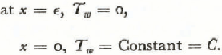
In Fig. 11, consider a semi-infinite ice mass whose bottom at time t = 0 was originally at x = 0 but at t = t is now at x = ϵ. In other words, in time t, a layer of ice of thickness, ϵ, has melted.

Fig. 11. Heating of an initially isothermal ice half-space over a warmer ocean, no melting
If Ki is the thermal (molecular) conductivity of ice, A is the eddy conductivity of sea-water and L is the heat of fusion of (fresh-water) ice, there is the following exchange of energy at the ice-water interface:
The temperature distributions in the ice and water will satisfy the Fourier heat conduction equations:
and
where A is assumed to be constant, and ρ w , and c w are very nearly equal to unity.
The solutions are given by
and
where the B’s and D’s are constant, and

The boundary conditions are
for ice:

for water:
Then, as shown by Neumann,Reference Neumann 31 the only non-trivial solution satisfying (4) and (5) and the boundary conditions, requires that
The solutions then become
and
where
By inspection (12) and (13) are seen to satisfy the boundary conditions (9) and (10). Differentiating (12) and (13) with respect to x and substituting in the energy exchange equation (3), we arrive at
If the temperature of the sea-water is everywhere “just above” the freezing point of sea-water (taken as 0° C. for convenience) then in (3) the term on the left side vanishes. If we assume further, that the energy used in melting the ice is exactly equal to that used in heating the ice, i.e.
which leads to Stefan’s solution,Reference Stefan 32 a special case of Neumann’s solution.
When (15) is solved for b and the value inserted in (12), it gives the solution for the first case, referred to in the preceding text, and is the equation from which curve “b” in Fig. 1 was drawn.
Equation (14) which does not assume uniform “freezing” temperature of the water nor equipartition of energy, gives the solution for the second case, and is the equation from which curves “c” and “d” in Fig. 2 were drawn. Since equation (14) is transcendental, the solution for b must be sought numerically after values have been substituted for the physical constants, K i , A, κ i , κ w , L, ρ i , and for the boundary temperatures, T 0 (of ice) and C (of seawater).
The curves of constant melt shown in Fig. 4 as functions of ΔT (deviation of sea-water temperature from its freezing point at x = 0) and A (eddy conductivity of sea-water), were drawn from (14) for t = 100 and 200 yr., under the assumption that T, the initial (and uniform) temperature of the ice shelf was 20.5° C. below the freezing point of sea-water (assumed for convenience in these calculations to be 0° C.). The parameter, b = ϵ/√t, is constant along a curve of constant melt. Since the thickness of the melted ice varies with √t, the curves in Fig. 4 may be re-labeled for any time, t yr., by multiplying the 100 yr. melt amounts by √t/10.
So long as one selects pairs of values, ΔT (or C) and A, from the same curve of equal melt in Fig. 4 (along which b is constant), the temperature distributions in the ice and water (x ≥ 0), Ti and Tw , for any time, t, will be the same regardless of the choice of ΔT or A, as may be seen by inspection of equations (12) and (13).


