2.1. GAP (γ-attenuation profiling)

The absorption and scattering of g-rays originating from a radioactive source (¹³⁷Cs) and passing in the transverse direction through the ice core to the detector (Reference WilhelmsWilhelms, 1996, 2000) are used for g-attenuation profiling. The radiation is monochromatic and thus the mass absorption coefficient is known with 0.1% relative error. The statistical intensity measurement errors of the free-air reference and at each sampling position are determined from direct analysis of the recorded data collection of at least 20 measurements. The calibrated detector signal is corrected for variations in core diameter. Furthermore, the possible influence at maximum misalignment of the core within the bench is estimated and a propagation of error is performed for each single measurement. The precision of the density measurement is typically in the range 0.006–0.01 gcm^–3 for a 100 mm diameter core. Unreliable data in the vicinity of core breaks are removed from the dataset. Along the EDML ice-core density was measured to 450 m depth in 5 mm increments (Fig. 1).

2.2. DEP (dielectric profiling)

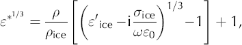
We express the complex parts of the relative dielectric permittivity as

(1)

where the real part, ɛ′, is the ordinary relative permittivity of the medium. The imaginary part, the dielectric loss factor, is related to conductivity, σ, and radian frequency, ω, by ɛ″ = σ(ɛ₀ω)^–1, where ɛ₀ is the permittivity of free space. Both parts of ɛ* can be determined with DEP (Reference Moore and ParenMoore and Paren, 1987). An improved DEP scanner (Reference WilhelmsWilhelms, 2000), operating at 250kHz, was used over the full depth of the EDML ice core (2565.55 m). The upper 12.6 m of the dataset are missing because of the operational set-up of the deep drilling. They are replaced by adjusted profiles of the shallow ice core B32, located 1.5km to the west. The calibrated DEP record is corrected for variations in core diameter and temperature. Unreliable data in the vicinity of core breaks, as for GAP, are removed. The correct interpretation of DEP requires that the effects of mixing of air and ice are taken into account. This is done by applying the formula for density and conductivity mixed permittivity (Reference WilhelmsWilhelms, 2005) explained below.

2.3. ECM (electrical conductivity measurements)

ECM is essentially a measure of d.c. conductance. It has traditionally been carried out by dragging a pair of electrodes with a high voltage between them along a core, and measuring the current between the electrodes (Reference HammerHammer, 1980; Reference Neftel, Moor, Oeschger and StaufferNeftel and others, 1985). A new ECM system, developed at the University of Bern, was used in the field at Dome Concordia (Reference Wolff, Basile, Petit and SchwanderWolff and others, 1999) and later in the laboratory for measuring the EDML ice core. In brief, a flat surface is prepared in the ice-core processing line along its full length using a horizontal band-saw and a microtome knife. The electrode assembly consists of seven electrodes at an inter-electrode spacing of 8 mm across the core. The electrodes are made of a carbon-doped silicon rubber. They are lowered onto the flat surface of the core and 350 V is applied across each adjacent pair of electrodes in turn. The current between the electrodes is sampled at regular intervals after a settling time, and averaged. The electrodes are lifted and moved 1 mm along the core and the sequence is repeated. This procedure yields six sets of data at 1 mm resolution. The data presented here are averaged over 10 mm and corrected to –15°C. Documented major core breaks and ends are removed from the ECM record. To date, corrected ECM data are available along the EDML ice core from 113.01 to 2563.98 m depth.

2.4. DECOMP (density and conductivity mixed permittivity)

Reference Kovacs, Gow and MoreyKovacs and others (1995) match a comprehensive dataset with a simple empirical formula relating the ordinary relative permittivity ɛ′ to density ρ: ɛ′ = (1 + 0.845ρ)². They obtain a standard error of ±0.031 for ɛ′, about 1% of the permittivity of pure ice (i.e. ice without bubbles and impurities). Reference LooyengaLooyenga (1965) derives a theoretical mixing model for air distributed in a dielectric medium based on spherical approximations of bubbles. Extension of his relation to complex space (Reference WilhelmsWilhelms, 2005) leads to

(2)

where the subscript ‘ice’ refers to values of the pure-ice (i.e. bubble-free) volume fraction, taking into account impurities that contribute to conductivity, like acids. Variables without a subscript refer to bulk values of the ice–air mixture. Reference WilhelmsWilhelms (2005) demonstrates that neglect of complex mixing for the density–permittivity relation could result in significant errors in ɛ*. Combination of γ-attenuation density and DEP data for the upper 450 m of the EDML core, analogously to Reference WilhelmsWilhelms (2005), yields and ρ_ice = 926 kgm^–3. Based on these values for the pure-ice fraction, which are the most consistent available for our site, we numerically invert Equation (2) to derive density and conductivity from the DEP measurements at 250 kHz (Fig. 1). Directly applying Equation (2) to the inverted DEP density and conductivity yields ɛ* at 150 MHz, assuming that ɛ’ does not change with frequency. This is done for the combinations of density (GAP and DEP) and DEP conductivity shown in Table 1. Each combination serves as input to a run of the wave-propagation model described below and results in a synthetic trace, designated S _i (i = 1, ..., 5) (Table 1). For ice, a Debye relaxation occurs below 10 kHz (Reference Bittelli, Flury and RothBittelli and others, 2004). Its tail causes a tiny frequency dependence of complex permittivity ɛ* in the MHz range (Reference Fujita, Matsuoka, Ishida, Matsuoka, Mae and HondohFujita and others, 2000, figs 2 and 3). Our calibration of the pure-ice permittivity described later implicitly takes care of this small effect for ɛ . Moreover, Equation (2) suffices to scale the conductivity with frequency, as the Debye relaxation frequency has been found to be constant near and at conductivity peaks (Wilhelms, unpublished data).

Table 1. Description of radargram origin

Fig. 2. Location of airborne profile 023150 and of ground-recorded profile 033042. The numbers refer to 10-fold stacked traces along profile 023150. The circle indicates the position of the EPICA drilling site. Reference radargram R ₁ corresponds to trace number 4204, which is closest to the drilling site. R ₂ is calculated from stacking all ~14 000 traces of profile 033042.

Fig. 3. Comparison of RES- and FD-radargram envelopes on a logarithmic scale (arbitrary units). From top to bottom: trace 4204 of profile 023150 (R ₁); 14 000-trace stack of profile 033042 (R ₂); nomenclature of synthetic radargrams (Table 1): plain symbols, S _i: ɛ′ = 3.09; primed symbols, indicates the filter length for ɛ′; specifically: S ₁ and S ₂ are based on DEP and GAP profiles, respectively, and using and a 0.2 m running mean filter applied to ɛ′ (indicated by l〈ɛ′〉); S ₃ and S ₄, which are the same as S ₁ and S ₂, respectively, but with a 20 m running mean filter applied to which is the same as S ₃, but using and based on DEP-density and ECM-conductivity profiles with and l〈ɛ′〉 = 20m. The magnitude of the synthetic radargrams is linearly scaled with travel time to compensate for the logarithmic pre-amplification of the RES system. Note the different scale of the 2–5 µs (the length of the GAP record) and 5–20 µs range.

ECM measurements along the EDML core were not carried out simultaneously with GAP and DEP, therefore restricting the use of Equation (2). An exact transfer of measured d.c.-ECM conductivity values to the frequency of radio waves requires knowledge of chemical composition and frequency-dependent properties of the constituents (Reference Moore, Wolff, Clausen, Hammer, Legrand and FuhrerMoore and others, 1992, 1994). Moreover, ECM is not a direct measure of electrical d.c. conductivity, as currents depend on the contact area of the electrodes which is difficult to keep constant, and are predominantly influenced by the conductivity in the vicinity of the contact area. ECM currents are also affected by electrode polarization (Reference Maidique, von Hippel, Knoll and WestphalMaidique and others, 1971). For our ‘proof-of-concept’ study, which is based on conductivity changes rather than on the absolute values, we choose a simpler approach. We scale the ECM record so that the mean ECM conductivity equals the mean DEP conductivity, the latter corrected for dielectric mixing and transferred to the MHz range, so that their means agree over the whole depth range. For all model runs S ₅ (Table 1) the DEP-conductivity data are then replaced by the scaled ECM-conductivity record.

3.1. Reference radargrams from airborne RES

We use RES data obtained with the Alfred Wegener Institute airborne system operated on the Polar2, a Dornier 228-101 aircraft, from Antarctic seasons 2002 and 2003. The system generates a 150 MHz burst of 60 ns duration with a peak power of 1.6 kW and 20MHz bandwidth (Reference NixdorfNixdorf and others, 1999). The receiver system includes a logarithmic amplifier and rectifies the received signal, i.e. the phase information is not recovered. An analog-to-digital converter samples at an interval of 13.33 ns and records over a window of 50 µs. Two hundred consecutive traces are stacked and the averaged traces are stored on tape. The overall system performance figure is 190 dB. During airborne surveys the ground speed is 65 ms^–1 (130 knots), resulting in a trace spacing of 6.5 m (Reference NixdorfNixdorf and others, 1999).

Two RES profiles are considered, the locations of which are displayed in Figure 2. Profile 023150 was recorded during flight at an altitude of 450 m. It runs parallel to the ice divide in an east-southeast–west-northwest direction and passes the drilling location at a distance of ~100m to the north-northeast. Horizontal stacking was applied to ensembles of ten consecutive traces stored on tape. The stacked trace 4204 is used as reference radargram R₁. To provide a higher spatial coverage and at the same time avoid uncertainties in the orientations of the airplane during flight, profile 033042 was recorded with the airplane sliding on the ground. An area of 200 x 300 m² about 500 m west- northwest of the drilling site was covered with some 14 000 traces recorded with multiple orientations of the airplane. Stacking of all traces results in the reference radargram R ₂. No additional filtering or gain control is applied to the RES data. The reference radargrams R ₁₂ (Fig. 3) are shifted in time such that their first break (the reflection from the surface) occurs at 0. We omit the time interval 0–2 µs as the strength of the surface reflection saturated the RES system receiver.

It is obvious from Figure 3 that the signal-to-noise ratio (SNR) in R₂ is remarkably lower than in R₁ because of the much higher stacking coverage. Despite the higher SNR, maximum amplitudes of reflections are slightly lower than for R₁ for two reasons. First, the profile 033042 covers an area that is larger than the first Fresnel zone of the transmitted wave. Second, the stacked traces were recorded with different antenna orientations, and thus did not take account of the anisotropic and birefringent properties of the ice (Reference HargreavesHargreaves, 1978; Reference Fujita, Matsuoka, Ishida, Matsuoka, Mae and HondohFujita and others, 2000). Both these contribute to destructive interference and thus lower amplitudes. At times >18 µs the reflections are very close to the system noise level, and result in a lower boundary in amplitude with no further decrease with travel time. In this interval, several reflections can be more clearly identified in R₂ than in R₁. Within each radargram a reflection maximum can be located with an uncertainty of one sample interval (±13 ns). The position of numerous major reflections, rising more than three times above the surrounding magnitude and present in each reference radargram, are in very good agreement with each other. The remaining differences in travel times of temporally corresponding reflections in R1 and R₂ are most likely caused by the 0.5 km separation of the locations. For the differences in travel time we obtain 0 ≥ Δt _R2—R1 ≥ —50 ns for travel times less than 10 µs, that is reflections of R ₁ occur slightly later than those of R ₂. For travel times beyond 20µs, 0 ≤ Δt _R2–R1 ≤ 80 ns, reflections of R ₁ occur earlier than those of R ₂.

3.2. Calculation of synthetic radargrams

We use a one-dimensional version of the parallelized finite- difference (FD) time-domain model successfully applied to the simulation of shallow ground-penetrating radar radargrams by Reference Eisen, Wilhelms, Nixdorf and MillerEisen and others (2003), which are based on the staggered-grid formulation of Maxwell’s curl equations (Reference YeeYee, 1966). The model operates with a spatial increment of 0.02 m and a time-step of 0.02 ns, ensuring numerical stability and dispersion criteria (Reference Eisen, Wilhelms, Nixdorf and MillerEisen and others, 2003). The data domain extends from 0 to 2565 m (the ice-core length). The model domain is chosen large enough that reflections from the model boundaries do not interfere with physical reflections caused by ice-core properties. Profiles of ɛ* at 150 MHz serve as model input, which are calculated from different combinations of DEP-, GAP- and ECM-based permittivity and conductivity data introduced above (Table 1).

The rectification and logarithmic amplification of the RES receiver signal prevents the phase retrieval of the signal transmitted into the ice. Theoretically, the 60 ns burst should contain nine sinusoidal waves of 150MHz. Hardware- related finite rise and decay times of the burst-trigger switches, common for RES transmitters (Reference Matsuoka, Saito and NaruseMatsuoka and others, 2004b), and the limited bandwidth of the transmitter antenna (Reference NixdorfNixdorf and others, 1999) lead to signal broadening and changes in the frequency spectrum. This is evident from the envelope shape of the received reflection from the air–ice interface. It has a total width of roughly 140 ns at half maximum, i.e. more than twice the theoretical pulse length (which partly results from reverberations of the surface).

Radargrams produced by wave-propagation modeling as well as real measurements are sensitive to the transmitted signal (e.g. Reference MinersMiners, 1998). Especially long wavelets easily lead to interference and reduced resolution; in the worst case even destructive interference. Unfortunately, the exact characteristics of the radiated wavelet of the airborne system are unknown. We have two aims: first, our main concern is to identify the depth of origin of a reflector at high resolution; and, second, we aim to determine the type of physical signal that causes the reflection. For the first aim a short synthetic source pulse should be used, as a long one could cause a degradation in the quality of the synthetic radargrams, which do not occur in the real measurements. However, our second aim requires a longer pulse, as a short one (e.g. a Ricker wavelet) could not reproduce the physical smoothing effect, i.e. interference, of a longer pulse. As a trade-off we use a synthetic wavelet consisting of only 2.5 150 MHz cycles of unit amplitude for modeling. In addition, half-wavelength oscillations of lower amplitude are added that precede and follow the synthetic wavelet, as is typical for burst and pulse radar systems (Reference Miners, Wolff, Moore, Jacobel and HempelMiners and others, 2002).

The following processing steps could be regarded as a filtering procedure that aims to conciliate our apparently incompatible aims. To synchronize the occurrence of maximum power of the RES direct coupling signal and the synthetic transmitter signal, the FD radargrams are shifted by +0.1 µs. Further processing includes application of a Hilbert magnitude transformation to the synthetic radargrams to obtain envelopes. Additional smoothing with a 100 ns Gaussian running mean filter adjusts the visual effect of the shorter FD-source signal to that of the broader RES reflection characteristics.

To reduce the effect of differences in resolution and statistical uncertainty of the various ice-core measuring devices on the synthetic results discussed below, we first apply a 2 cm running mean to all input data. This filter length is below the typical peak width of conductivity signals (e.g. from volcanic eruptions). Statistical noise is thus reduced, but the signal is preserved. The characteristics of ε′ show fluctuations at scales of centimeters to decimeters. As will be shown next, these are related to the measurements so that additional filtering is necessary to recover the reflections present in the RES reference radargrams.

3.3. RES vs FD: the role of ε′

Over the whole travel-time range of 2–26 µs the comparison of the synthetic radargram S ₁ calculated from DEP data, with an additional 0.2 m running mean filter applied to ε′ (Table 1), shows few features in common with the RES reference radargrams R ₁₂ (Fig. 3). However, the synthetic radargram S ₃, based on ε′ data filtered with a 20m window and ε″ data with a 0.02 m running mean, contains several events which are found in both reference radargrams. The higher variability in S ₁ reflectivity relative to that of radargram S3 implies that the density signal underlying S1 is too noisy to reproduce reflections present in RES radargrams. Moreover, the stronger decrease of reflected magnitude in S ₁ with travel time beyond 10µs in comparison to S ₃ indicates that the unrealistic noise present in ε′ produces higher reflection loss, meaning that less energy is transmitted to deeper ice.

A second set of numerical modeling runs based on the GAP-density and DEP-conductivity records in the depth range 0–450m (a time range of 5 µs) produces the same result (S ₂ and S ₄ in Fig. 3). Despite the different origin of the GAP-density data, low-pass filtering on the order of tens of meters of ε′ (S ₄) is necessary to achieve an agreement in the reflection pattern, with the synthetic radargram S3, as well as the reference radargrams R ₁ and R ₂. Therefore density signals derived from either DEP or GAP contain too much noise to reproduce radargrams with a sufficiently high SNR for regions below the firn–ice transition, in a depth range where conductivity signals become important. In the remaining part of the paper we consequently restrict our RES–FD comparison to synthetic data for which ε′ has been filtered over 20 m. Note that the smoothing has a negligible influence on the travel-time–depth relation (which depends on integrated ε′’);it merely improves the quality of reproduced reflections.

3.4. RES vs FD: characteristic peaks and time shift

A number of reflection patterns visible in the RES reference radargrams R ₁ and R ₂ are reproduced in the synthetic radargram S3 (Fig. 3). However, the synthetic reflections in S ₃, which is based on occur earlier than the corresponding RES signals. To reduce this systematic time shift we model another set of synthetic radargrams i = 3, 5 (Fig. 3), based on ɛ* calculated with in the forward mixing application at 150 MHz of the DECOMP formula (2). Possible reasons for this observation will be discussed below.

A cross-correlation analysis of the synthetic radargrams with the reference radargrams (denoted by S × R) for the time interval 10–26 µs demonstrates the improved agreement (Fig. 4). (As density variations contribute to reflections down to 10 µs, extending the cross-correlation to shorter travel times includes the uncertainty related to density measurements and leads to less clear results, but is nevertheless feasible.) Prior to cross-correlation all synthetic and RES radargrams are unified to a common sample interval of 1 ns by linear interpolation. The cross-correlation is applied to the logarithmic magnitudes, which are, in the case of the synthetic radargrams, linearly scaled with time to compensate for the RES system’s pre-amplification, and for the progressive decrease of magnitudes caused by geometric spreading and losses. The cross-correlation function of S ₃ × R ₁ and S 3 × R ₂ has a broad maximum (Fig. 4). S ₃ leads R ₁ and R ₂ by 164 and 153 ns, with correlation maxima of 0.69 and 0.65, respectively. The cross-correlation of S3 × R ₁ and S ₃ × R ₂ results in slightly changed maximum correlation coefficients of 0.64 and 0.66, respectively. However, the time shift now changes to a lag of with respect to R ₁ and R ₂ of 36 and 12 ns, respectively, that is only 1–3 RES sample points. Moreover, the cross-correlation function related to shows a more pronounced peak of maximum correlation than is the case for S3. Based on these results, the in situ travel time underlying the RES radargrams appears to be about 1.6% lower than that arising from the ice-core data in the synthetic radargrams. To identify the originating depth of reflections, our main goal, we use ice-core data processed with for our further modeling. The related synthetic traces are marked with primed symbols ( where only i = 3 and 5 will be used; see Table 1).

Fig. 4. Cross-correlation functions of S ₃ (ɛ′_ice = 3.094) and (ɛ′_ice = 3.20) with R ₁ (thin line) and R ₂ (thick line) for the time interval 10–26 µs with a maximum lag of ±500 ns.

Several sections of show exceptionally good agreement with R ₁ and R ₂ (Fig. 5) Most prominent are the series of signals at 5–6 µs and 19.5–20.5 µs, the double peaks at 12.6 and 13.7µs, and the single events at 7.2, 7.7, 10.2, 15.5, 18.4, 22.1 and 24.7µs. Not only do the times of the reflections correspond to each other, in several cases their structures are also similar. For example, the narrow double peak at 12.6 µs, almost at the limit of temporal resolution in the RES radargrams, is reproduced in the synthetic radar- gram. Distressingly, the synthetic reflection at 21.1 µs occurring in has no counterpart in R ₁ or R ₂. Possible reasons are discussed at the end of section 4.3.

Fig. 5. Comparison of RES- and FD-radargram envelopes on a logarithmic scale in arbitrary units. For nomenclature of FD radargrams see Table 1. On top of (black) radargram (gray) is plotted. Reflections not present in therefore appear black. The same is the case for and Dominant reflections mentioned in the text are enframed by gray dotted lines. Black boxes on the x axis indicate truncated conductivity peaks used in and No time- variant scaling is applied above 18 µs. Beyond 18 µs the square root of magnitudes multiplied by travel time is displayed to compensate for logarithmic pre-amplification and decreasing SNR of the reference radargrams.

To investigate the reproducibility of the above comparison based on DEP conductivity, we calculate another synthetic radargram, based on ECM conductivity ( Table 1). The reflection sequences (Figs 3 and 5) are in general very similar to , especially at 5–6, 7.7, 10–12, 12.6, 13.8, 15.5, 18.4, 19.5 and 22.1 µs. However, the reflections resulting from ECM conductivity are less significantly greater than the background variability, compared to the reflections from DEP conductivity (e.g. at 12.6 and 15.5 µs). The low amplitudes of around 7.3 µs are caused by missing ECM data. The reflections produced by DEP conductivity at 19.8–20.5 and 24.7 µs are not reproduced by the ECM conductivity.

4.1. Depth and type of reflector origin

Having identified a number of reflections in the reference radargrams that are reproduced in the synthetic radargrams, we now proceed to determine the physical origin of the synthetic peaks, and thus their originating depth. A correlation between conductivity and reflections has been demonstrated by other studies (Reference Hempel, Thyssen, Gundestrup, Clausen and MillerHempel and others, 2000; Reference Miners, Wolff, Moore, Jacobel and HempelMiners and others, 2002). We therefore test if individual conductivity peaks present in the DEP and ECM data are also responsible for the strong reflections. (Remember that the permittivity for all S ₃ radargrams is smoothed so that all synthetic reflections should be caused only by conductivity signals.) A number of strong conductivity peaks in the ɛ* profile are removed (Table 2). The gaps are then closed by linear interpolation (Fig. 6). All of the considered conductivity peaks rise about 2–5 times above the background conductivity of ~10 µSm^–1, are less than 0.5 m wide and are most likely of volcanic origin. The synthetic radargrams calculated from these data with truncated conductivity peaks (denoted with a tilde, and ) lack a number of the prominent reflections present in and respectively, which have counterparts in the RES radargrams (Fig. 5). For clear correspondence occurs for the reflections at 7.2, 7.7, 12.6, 13.7, 15.5, 18.4, 22.1 and 24.7 µs. In these unambiguous cases the good agreement between synthetic and reference radargrams and the identification of reflection origins enables us to relate the travel time observed in the RES radargrams to the depth of the removed single conductivity peaks. For the agreement and effect of the truncation is somewhat different. Unambiguous cases occur at 12.6 and 19.5 µs. The RES travel times are taken from R₁ , as this radargram stems from a continuous long-distance profile which is closest to EDML, in contrast to the spatially confined radargram R ₂. We determine the travel time at maximum amplitudes for ten reflections (Table 2). They are accurate with respect to other reflections to within one sample interval, in our case 13 ns.

Table 2. Travel-time–depth relationship for selected reflections from trace R ₁

Fig. 6. DEP-conductivity peaks (black) for the depth range 800–2100 m (~10–25 µs), considered in the sensitivity study to calculate for comparison with The peaks are removed and the gaps subsequently linearly interpolated (gray), plotted on top of the original curve. Each x-axis segment covers 1 m depth with ticks every 0.1 m.

Two observations indicate not only that single large conductivity peaks cause reflections, but that constructive interference between reflected signals also occurs. The reflections at 18.4 and 22.1 µs require that a series of two and three conductivity peaks, respectively, has to be truncated to completely remove the reflections (Table 2). Interpolation of only one peak of the series merely results in a reduced amplitude of the corresponding reflection. In other cases, the truncation of conductivity peaks does not lead to a significant change in the reflection structure. For instance, the reflection sequence in the range 5–6µs, the three broad reflections from 19.5 to 20.5 µs and the single reflection at 10.2 µs.

4.2. Error analysis

The accuracy of the established travel-time–depth relations differs for the different types of reflections selected here. According to Ricker’s criterion for resolution limits, two signals can be resolved if the separation of their maxima is larger than the full width at half maximum. The RES reflections typically have a full width at half maximum of some 50 ns travel time, which corresponds to about 4m depth in solid ice. For the processed synthetic traces this value is around 25 ns or 2 m, the higher accuracy because of the shorter source wavelet. Where a single strong conductivity peak causes a synthetic reflection which is in accordance with the RES radargrams, the relation of reflection travel time and reflector depth is unambiguous. The centers of the conductivity peaks in the DEP profile are taken as the depths of origin of the reflections, and the peak width determines the accuracy in depth (Table 2). As all conductivity peaks are less than 0.5 m wide, the error of the depth estimate is less than ±0.5 m. This accuracy cannot be achieved for reflections stemming from constructive interference occurring at closely spaced conductivity peaks, such that the resolution criterion given above is not fulfilled. Nevertheless, it is still possible to pin down the depth of origin, though with a larger uncertainty. The two conductivity peaks related to the reflection at 18.4 µs are separated by 1.1 m and together cover a total depth range of 1.3 m, implying a depth estimate accurate to within ±0.7 m. The series of three peaks from 1866.5 to 1869.6 m are separated by at most 1.9 m and cover a range of 3.1 m, which is still smaller than the possible resolution of the RES radargrams. In other cases, for instance for the groups of reflections around 5.3 and 19.5–20.5 µs, several meters of the conductivity profile have to be truncated to completely remove the reflection signature. The uncertainty of the depth estimates in these cases ranges from 2 to 5 m, depending on the profile structure.

4.3. Comparison to other methods

Usually a certain wave-speed–depth function is integrated from the surface to a certain depth to determine the relevant travel time. As any wave-speed estimate is subject to an error, the integration results in an increasing absolute uncertainty with increasing travel time and depth and thus also for the subsequent travel-time–depth conversion. A relative error in wave speed is linearly translated into an equivalent error in depth.

The method introduced here significantly reduces this relative uncertainty by correlating synthetic and RES radargrams in the time domain based on reflection patterns to identify the reflection origin in the depth domain of the ice-core data. Given the physical properties, the model produces the reflections at the right position and enables us to accurately connect reflectors and ice-core properties. Our travel-time–depth relationship is subject to an absolute uncertainty, which mainly depends on the quality of correspondence between the RES and synthetic reflections. Simultaneously, it takes into account the small depth- dependent variations of wave speed. Given a 1% uncertainty in measured wave speeds (a realistic estimate as demonstrated in Fig. 1), the corresponding depth uncertainty for an ordinary travel-time–depth conversion will likewise be 1%, increasing from 1 m at 100 m depth to 20 m at 2000 m depth. In contrast, our travel-time–depth relationship established above is only subject to an absolute error on the order of 1 m, independent of depth. This simple example illustrates that our method is therefore especially useful for deeper reflections.

A tough constraint for reliable functionality is put on the method by the high SNR demanded of RES and synthetic radargrams. As demonstrated, RES data with high SNR can be produced by increased spatial and temporal coverage. Whereas this is no problem for ground-based surveys, it might not be always possible during airborne measurements.

In polar ice, reflection coefficients for electromagnetic waves at radio frequencies are dominated by changes in ɛ″ and are less sensitive to impedance contrasts of ɛ″. Masking of most reflections originating from conductivity peaks in the synthetic radargrams by noise in the density profiles can be overcome by low-pass filtering of ɛ;. Unfortunately, this also eliminates the information related to small-scale variations in ɛ′ (from permittivity or anisotropy) in the synthetic radargram. This explains why the agreement of RES and synthetic traces is better below 10 µs than above.

In general, core breaks or only a few centimeters of cracks could also easily mask reflections from conductivity peaks or lead to a rejection of a core section in the quality check. Apart from the difference in conduction mechanisms, this is probably one reason why some reflectors appear in the DEP radargrams, but not in the ECM radargrams (e.g. at 19.8–20.5 and 24.7 µs Fig. 5). In addition, it can also happen that reflections in the reference radargrams are not reproduced by the DEP or the ECM conductivity. As recently shown by Reference Wolff, Cook, Barnes and MulvaneyWolff and others (2005), it is difficult to reproduce the conductivity profile for replicate ice cores. In their study at Dome Concordia, two 800 m long conductivity profiles of two ice cores 10 m apart do reproduce individual peaks, but their magnitude varies, typically by a factor of 1.5. Some signals are even completely missing in one of the cores. It is therefore unlikely that synthetic radargrams will reproduce all the RES radargram peaks, even if the measurements take place at exactly the same location, and more so if the locations are separated by a few tens to hundreds of meters.