


1. Introduction
Fast-moving glaciers move predominantly by slip along the glacier sole, which largely controls the rate at which outlet glaciers discharge ice into the ocean (Rignot and others, Reference Rignot, Mouginot and Scheuchl2011) and contribute to sea-level rise. For accurate forecasts of glacier contributions to sea-level rise, process-based parameterizations of glacier slip need to be implemented in large-scale ice-sheet models (e.g. Ritz and others, Reference Ritz2015; Pollard and Deconto, Reference Pollard and Deconto2016; Kopp and others, Reference Kopp2017). Importantly, hard-bedded (i.e. bedrock) regions of glaciers may supply disproportionately large basal drag compared to soft-bedded (i.e. sediment) regions (Koellner and others, Reference Koellner, Parizek, Alley, Muto and Holschuh2019; Maier and others, Reference Maier, Humphrey, Harper and Meierbachtol2019, Reference Maier, Gimbert, Gillet-Chaulet and Gilbert2021; Muto and others, Reference Muto2019) owing to the higher effective stresses commonly sustained in hard-bedded areas (Tulaczyk and others, Reference Tulaczyk, Kamb and Engelhardt2000). Incorporating improved hard-bed slip parameterizations in large-scale ice-sheet models would help improve estimates of glacier discharge.
Slip behavior can be generalized with a slip law that relates the magnitude of basal drag (τ b) acting on the glacier sole to a given slip velocity (u s) or effective pressure (N, overburden pressure minus water pressure). Attempts to estimate the form of the slip law started with the ‘tombstone’ model of Weertman (Reference Weertman1957). This model describes glacier slip resulting from regelation and viscous creep around rigid, cubic obstacles at the bed (Weertman, Reference Weertman1957). The resulting slip law, which has been widely used in modern ice-sheet models (Larour and others, Reference Larour, Seroussi, Morlighem and Rignot2012; Nick and others, Reference Nick2013; DeConto and others, Reference DeConto2021), has a power-law form with unbounded basal drag at a given effective pressure (τ b/N) as u s increases (Fig. 1). However, in addition to its unrealistic bed geometry, this model does not describe the effects of ice-bed separation in the lee of bed obstacles (i.e. cavities), which reduces the area of ice-bed contact, thereby affecting τ b (Fig. 2).
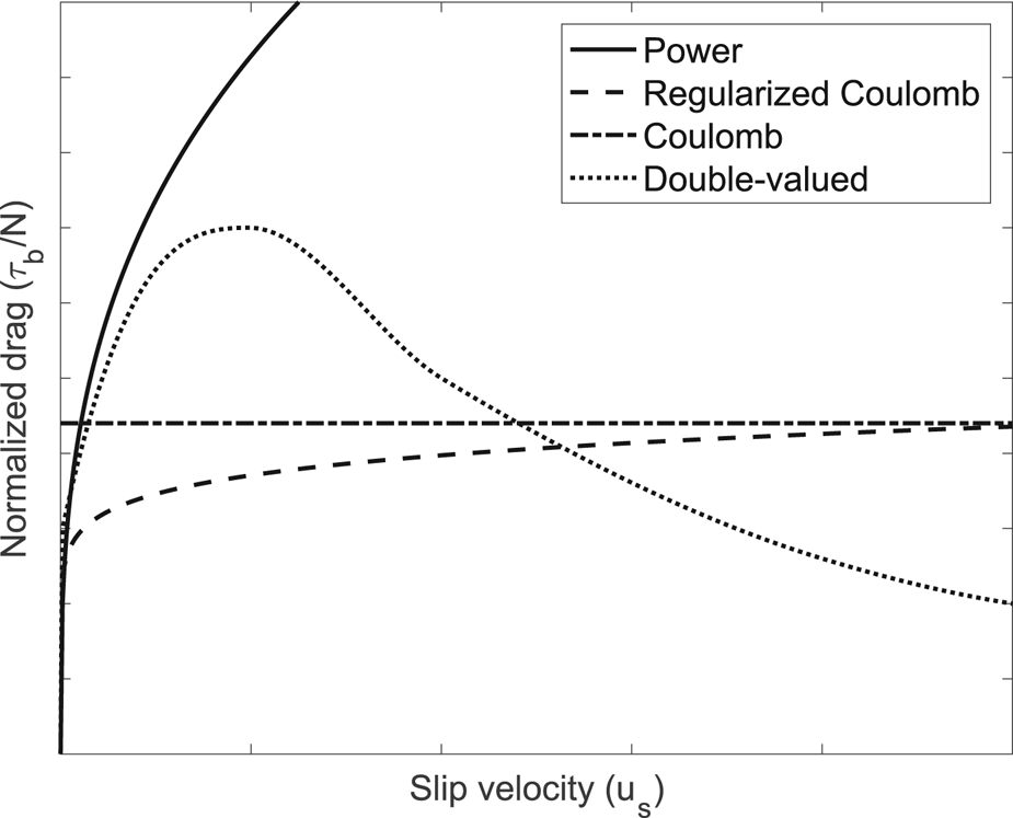
Fig. 1. Illustration of different slip-law forms that show the change in normalized drag (τ b/N) with slip velocity (u s).

Fig. 2. Treatment of subglacial cavities. (a) An idealized representation of the bed geometry (blue line), cavity geometry (green line) and the areas of ice bed contact (red line). Variables used to calculate the shadow function are also illustrated (see methods). (b) Example of an along-flow bed profile from Schwarzburg illustrating the estimated cavity geometries (green lines), cavity detachment points (red stars), reattachment points (blue circles) and periodic wrapper (black squares). Ice flow direction is from left to right along the horizontal axes.
More recently, laboratory experiments (Zoet and Iverson, Reference Zoet and Iverson2015) and process-based models (Lliboutry, Reference Lliboutry1968; Fowler, Reference Fowler1987; Schoof, Reference Schoof2005; Gagliardini and others, Reference Gagliardini2007; Helanow and others, Reference Helanow, Iverson, Zoet and Gagliardini2020) based on idealized, periodic morphologies yield a ‘double-valued’ slip law (Fig. 1). That is, τ b/N increases with u s (rate-strengthening slip) up to some threshold, above which τ b/N decreases (rate-weakening slip). The double-valued slip law results from the change in bedrock slope in areas of ice-bed contact as cavities grow with increasing slip rates. For a simple sinusoidal bed, rate-strengthening occurs as the leeside ice cavities grow and ice-bed reattachment points approach the inflection points of the stoss bump surfaces immediately downstream, thereby increasing the mean bed slope in contact with the ice (Fig. 2). Rate-weakening slip behavior begins when the ice reattachment point extends beyond the sinusoidal bed's inflection point, decreasing the mean slope of the bed in contact with the ice with further cavity growth. These more recent process-based models neglect regelation, which is justifiable owing to the observed rarity of short bump wavelengths (<0.5 m, Hooke, Reference Hooke2020). Although slip models with ice-bed separation have been shown to be largely correct for their simplified geometries (Zoet and Iverson, Reference Zoet and Iverson2015, Reference Zoet and Iverson2016), their viability for more realistic irregular bed geometries was uncertain.
Process-based numerical models of slip with ice-bed separation provide slip laws for measured three-dimensional (3-D) bed geometries (Helanow and others, Reference Helanow, Iverson, Woodard and Zoet2021) and demonstrate that the rate-weakening slip associated with idealized, periodic beds is unrealistic. In contrast to slip laws for sinusoidal beds, numerical results for 3-D bedrock topographies from four recently exposed proglacial areas demonstrate that their associated slip laws are best described by a regularized Coulomb relation (Joughin and others, Reference Joughin, Smith and Schoof2019), where τ b/N increases toward a limiting value (Helanow and others, Reference Helanow, Iverson, Woodard and Zoet2021) (Fig. 1). This slip behavior arises from the irregular along-flow bed morphologies of actual beds, which prevent widespread reduction of bed slopes in contact with the ice with increasing cavity size. Importantly for this study, these modeling results demonstrate that variations in computed basal drag closely correlate with variations in the mean along-flow slope of the bed in areas of ice-bed contact,$\;{\bar m}$ . Thus, by determining the mean bed slope in areas of ice-bed contact, ${\bar m}$
 , at variable u s or N, the form of the slip law can be inferred.
Here we present a method for estimating the extent of cavities on an irregular 3-D bedrock surface, so the mean along-flow slope of the bed in contact with ice can be estimated. The method avoids computationally expensive numerical simulations (Helanow and others, Reference Helanow, Iverson, Woodard and Zoet2021), so it can be readily applied to large areas. We apply the method to 618 high-resolution (10 cm), 20 × 20 m, digital elevation models (DEMs) of bedrock topography from four proglacial areas. We first describe the field sites and measurements of bed topography and then discuss the method for estimating the mean slope of the bed in contact with the ice. We compare the results to those indicated by 3-D modeling of cavity geometry during glacier slip (Helanow and others, Reference Helanow, Iverson, Woodard and Zoet2021). This comparison allows us to infer the slip-law forms for all bedrock subsections spanning the proglacial areas.
2. Methods
2.1. Digital elevation models
Proglacial bedrock areas in the Swiss Alps and Canadian Rockies, exposed by glacier recession, are surveyed using photogrammetry techniques and a terrestrial laser scanner to create 0.1 m resolution DEMs (Fig. 3). Tsanfleuron, Schwarzburg and Rhône glaciers are located in Valais Canton, Switzerland, and consist of limestone, granitic gneiss and granite bedrock, respectively (Fig. 4a). Castleguard is a limestone-bedded glacier in Alberta, Canada (Fig. 4b). The survey designs, methods for DEM creation and determination of ice flow vector fields are detailed in Helanow and others (Reference Helanow, Iverson, Woodard and Zoet2021). To examine the full range of slip-law forms expected over a variety of bed topographies available in the proglacial areas, the DEMs are divided into 20 × 20 m adjacent grid sections oriented so that the mean ice flow direction of the section, as determined from striation orientations, is from left to right along the x-axis. Sensitivity analyses show that adjustments in the ice flow direction by up to 30° have little effect on the inferred slip-law forms (Fig. S1). The DEM subsection dimensions were chosen to include expected cavity lengths based on slip rates and effective pressures of mountain glaciers (Cuffey and Paterson, Reference Cuffey and Paterson2010). The subsections are detrended and tapered on both their upstream and downstream margins to assure periodicity in the along-flow direction while leaving most of the subsection unmodified. We adopt a different tapering method than Helanow and others (Reference Helanow, Iverson, Woodard and Zoet2021) for computational efficiency and because our new method of estimating ${\bar m}$ considers only the along-flow shape of the bed. A Tukey (tapered cosine) window is applied by subtracting the mean elevation from the along-flow profile, applying the Tukey taper (0.4 cosine fraction), then adding back the previously subtracted mean elevation to the profile. Comparing the estimates of ${\bar m}$
 between the Tukey taper and the taper used by Helanow and others (Reference Helanow, Iverson, Woodard and Zoet2021) indicates that the Tukey taper results in comparable slip-law forms (Figs S2 and S3). Detrending the subsections may change the magnitudes of the bed slopes but will not affect the form of the estimated slip laws. The tapering is required to permit cavity growth beyond the boundaries of the subsection and to simulate cavity formation over an infinitely long, repeating subsection morphology (see Fig. 2).

Fig. 3. Shaded relief map of the four proglacial areas: (a) Tsanfleuron, (b) Schwarzburg, (c) Rhône and (d) Castleguard. The mean ice flow direction for each proglacial area is from left to right.

Fig. 4. Locations of the four proglacial areas studied.
2.2. Estimation of average bed slope in contact with ice
To estimate the average slope in contact with the ice, ${\bar m}$ , we apply a cavity roof trajectory to each row (i.e. along-flow profile) of a proglacial DEM subsection, z(x, y). The slope of the cavity roof trajectory is dictated by the prescribed slip velocity, u s, effective pressure, N, and bed topography. From these roof trajectories we find the segments of each along-flow profile in contact with the ice (Fig. 2). The ice-roof trajectories can be thought of as oblique rays that ‘illuminate’ the bed profile where the ice and bed are in contact – similar to the ‘shadow’ function proposed by Lliboutry (Reference Lliboutry1968, Reference Lliboutry1979). Compiling the results from each profile of the DEM subsection, we determine the areas of the bed in contact with the ice and their average along-flow slope, ${\bar m}$
 . This method of determining ${\bar m}$
 neglects transverse strain rates and variations in mean slope of the cavity roof expected with different bump sizes along the profiles (Lliboutry, Reference Lliboutry1968). We do not use the model in Lliboutry (Reference Lliboutry1979) for determining the ice roof trajectories because the results vary significantly from the numerical solutions in Helanow and others (Reference Helanow, Iverson, Woodard and Zoet2021) (Fig. S4).
We determine the average slope of each profile's cavity roof by adapting the cavity geometry derived by Kamb (Reference Kamb1987) for 1-D sinusoidal profiles. Kamb's analytical model incorporates the non-linear rheology of ice but neglects the effects of basal melting and regelation. However, his solution for cavity geometry closely matches observations from lab experiments (Zoet and Iverson, Reference Zoet and Iverson2015). Although our profiles are not perfectly sinusoidal, approximating them as such to derive the slope of the cavity roof provided reasonable results. Following Kamb (Reference Kamb1987) the cavity length, l, of a sinusoid of wavelength λ and amplitude a is given by

where E is the wave cavitation parameter:

The parameter n is the stress exponent of the ice flow law (Glen, Reference Glen1952), taken to be 3.0, e is Euler's number and B is the viscosity parameter (Hooke, Reference Hooke2020). The value of λ is considered to be the profile wavelength with the highest spectral power (i.e. most variance) and is determined using the power spectral density of the bed profile. In the majority of the profiles (91%), λ was approximately equal to the largest wavelength (20 m). The dependence of λ on the dimensions of the subsection, among other simplifications, restricts the comparison to only the form of the slip law and not the magnitude of basal drag. Since λ is near the largest wavelength for most profiles, a is set to be half the profile relief range (half because of the sinusoid amplitude). The methods for choosing a and λ are heuristic, but by using the highest relief amplitude and the wavelength with the highest spectral power, we approximate the geometries of cavities with the greatest potential for shadowing the bed and thereby influencing ${\bar m}$ . Variation in these parameters would change the magnitude of ${\bar m}$
 with slip velocity but not the overall slip law form. Power spectral density, P(k), of the profile is estimated with the discrete Fourier transform periodogram (Press and others, Reference Press, Flannery, Teukolsky and Vetterling1986; Perron and others, Reference Perron, Kirchner and Dietrich2008):


Here k is the wavenumber, k = (2π/λ), j is the index of the profile, M is the number indices within the profile, W is the Hann tapering window and Z(k) is the discrete 1-D fast Fourier transform of the profile. The detachment point of the cavity roof, x o, is located a distance (3/8)l upstream from the sinusoid's inflection point (Kamb, Reference Kamb1987) and the reattachment point, x c, is located a distance l downstream from x o (see Fig. 2). The profile height at points x o and x c of a pure sinusoidal function of the form z o(x) = acos (kx) is used to calculate ${\bar s}$ of the cavity roof:

To determine ${\bar m}$ , we estimate the geometry of the cavity roofs by applying a ray tracing technique with the rays projecting with a slope ${\bar s}$
 and the areas illuminated by the rays representing areas of ice-bed contact. This procedure is carried out for each profile of a DEM subsection over a range of u s at a specific N. Computing the average slope of segments of ice-bed contact for z(x, y) must take into account the length of the contact areas for each profile. As such, we estimate the total length of the ice-bed contact segments of a profile within a DEM subsection, S, to determine ${\bar m}$
 :
:

where i is the profile index, m is the mean slope of the profile's ice-bed contact segments and i o is the total number of along-flow profiles (i.e. rows) in the DEM subsection.
Our first objective is to test this method for estimating ${\bar m}$ by applying it to the same representative subsections of proglacial topography where basal drag and ${\bar m}$
 were calculated using a 3-D full-Stokes simulation of cavity geometry during glacier slip in Helanow and others (Reference Helanow, Iverson, Woodard and Zoet2021). Assumptions made in this modeling were a free-slip boundary at the ice sole, uniform water pressure in the cavities, temperate ice and negligible effects of basal melting and regelation (see Helanow and others (Reference Helanow, Iverson, Woodard and Zoet2021) for more details). To compare values of ${\bar m}$
 with those calculated numerically by Helanow and others (Reference Helanow, Iverson, Woodard and Zoet2021), we use the normalized slip velocity, u s/N n. Values of N and B considered are 0.4 MPa and 73.3 MPa s1/3 (Cuffey and Paterson, Reference Cuffey and Paterson2010), respectively. Although the values of B at each site could vary (Chandler and others, Reference Chandler, Hubbard, Hubbard, Murray and Rippin2008), these differences would not affect the slip-law form estimated with the new method or the numerical model. As in Helanow and others (Reference Helanow, Iverson, Woodard and Zoet2021), we consider velocities of 0–100 m a−1 and use the same 3-D edge tapering, detrending and topographic filtering of representative subsections as in that study, to allow a valid comparison of the two approaches for estimating ${\bar m}$
 (Fig. 5). All other subsections were adjusted as described in section 2.1 for computational efficiency while maintaining good agreement with the numerical results (Fig. S2 and Fig. 6).

Fig. 5. Average bed slope, ${\bar m}$ , in contact with ice, as a function of scaled slip velocity, computed from full-Stokes modeling of basal cavities (Helanow and others, Reference Helanow, Iverson, Woodard and Zoet2021) and estimated with the new method. Also shown are values of τ b/N calculated by Helanow and others (Reference Helanow, Iverson, Woodard and Zoet2021). Results are for morphologically representative subsections of the (a) Tsanfleuron, (b) Schwarzburg, (c) Rhône and (d) Castleguard proglacial areas with the 3-D taper described in Helanow and others (Reference Helanow, Iverson, Woodard and Zoet2021).

Fig. 6. Average bed slope, ${\bar m}$ , as a function of scaled slip velocity for all surveyed subsections of the (a) Tsanfleuron, (b) Schwarzburg, (c) Rhône and (d) Castleguard proglacial areas, estimated using the new method. Solid black lines show the median ${\bar m}$
 values and the dashed black lines show the interquartile range. Bold lines highlight the individual DEM subsections that deviate from a regularized Coulomb slip law.
3. Results
Our method for estimating mean bed slopes in contact with the ice successfully approximates ${\bar m}$ computed from the 3-D numerical slip modeling of Helanow and others (Reference Helanow, Iverson, Woodard and Zoet2021). Figure 5 shows the estimates of ${\bar m}$
 from our method (red line) and the numerical model (black solid dots) using the 3-D taper described in Helanow and others (Reference Helanow, Iverson, Woodard and Zoet2021). Also shown in Figure 5 are the τ b/N values computed in Helanow and others (Reference Helanow, Iverson, Woodard and Zoet2021) (black open circles) to illustrate the strong correlation between ${\bar m}$
 and τ b/N. However, there is not a one-to-one correspondence between these values, indicating that ${\bar m}$
 cannot be used to directly estimate the magnitude of τ b/N. The magnitude of ${\bar m}\;$
 and its dependence on the scaled slip velocity are very similar for the two methods, indicating that the new method is an effective alternative for estimating the form of the slip-law. The greatest discrepancy is for the Tsanfleuron subsection, where the numerical solutions show slight rate weakening, but the new method indicates a regularized Coulomb form (Fig. 5).
The overall success of this relatively simple method for estimating ${\bar m}$ and the correlation between ${\bar m}$
 and τ b/N determined by Helanow and others (Reference Helanow, Iverson, Woodard and Zoet2021) (Fig. 5) makes it possible to infer the slip-law forms in more areas, so we now consider the results of applying the new method to 618 unique DEM subsections. The majority of them exhibit ${\bar m}$
 values that increase toward a limiting value (Fig. 6). The range of ${\bar m}$
 values for each proglacial subsection varies among the proglacial areas, with Tsanfleuron presenting the lowest median values (black line), and Rhône displaying the highest median values. Additionally, within a given proglacial area, ${\bar m}$
 values of subsections are variable, as shown by the 25th and 75th percentile bounds (dashed lines). Castleguard displays the narrowest ${\bar m}$
 bounds. The other DEMs have a few subsections with notably high ${\bar m}$
 values, but most subsections fall within a limited range (Fig. 6). Additionally, some of the proglacial areas contain a few subsections (~2% of all the subsections) that display a non-Coulomb slip relation (i.e. rate-weakening or rate-strengthening) at high velocities (bold colored lines), but otherwise proglacial subsections exhibit regularized Coulomb slip (Fig. 6).
4. Discussion
The general agreement between the estimates of ${\bar m}$ from the numerical model of Helanow and others (Reference Helanow, Iverson, Woodard and Zoet2021) and our new method indicates that our simpler method can approximate the more complete physics of the numerical slip model for estimating cavity geometry and the form of the slip law. However, the new method does not include the transverse component of ice flow, local variations in glacier slip velocity and variations in cavity closure rates on bumps of different sizes and shapes. The success of the method, despite these simplifications, implies that transverse strain rates and local variations in slip velocity tend to have a small effect on cavity geometries and associated spatial distributions of ice-bed contact. The success of the method may also reflect, in part, the extensive shadowing effects of larger bumps, which result in large cavities with roof slopes that are well approximated by the new method. Smaller bumps with cavity-roof slopes that are less accurately modeled with the new method tend to be drowned in larger cavities or, if not drowned, create cavities that affect only small areas of the bed. The least agreement between the numerical results and those of the new method is from Tsanfleuron, where the numerical model indicates slight rate-weakening slip. However, Helanow and others (Reference Helanow, Iverson, Woodard and Zoet2021, their Fig. S7) showed that for this domain the sensitivity of the model results to the details of the domain-tapering algorithm was too high to distinguish the computed slight rate-weakening from a regularized Coulomb slip relation. Thus, the results obtained with our method fall within the uncertainty of the results of the numerical modeling. Additionally, both the numerical model and the new method omit the effects of debris in the basal ice being in frictional contact with the rock-bed. However, the effects of this omission are likely minimal (see Iverson and others, Reference Iverson, Helanow and Zoet2019).
The consistent regularized Coulomb form of the slip laws across the proglacial areas is due to the similarity of the proglacial bed topographies (Woodard and others, Reference Woodard, Zoet, Iverson and Helanow2021). For instance, the narrow range of the magnitude of ${\bar m}$ at Castleguard (Fig. 6) reflects the uniformity of the stepped topography within that proglacial area (Fig. S5) (Hallet and Anderson, Reference Hallet and Anderson1980). There are some subsections of proglacial areas with bed topographies that result in non-Coulomb behavior at high velocities. Examples of topographies that produce the different slip-law forms are shown in Figure 7. The large, isolated bump in Figure 7a likely causes the rate-weakening behavior because it has the same convex shape as the sinusoidal bed that produced the double-valued slip law in experiments (Zoet and Iverson, Reference Zoet and Iverson2015, Reference Zoet and Iverson2016). As cavity size increases, the contact area is confined to areas near the bump's convex crest, causing the reduction in ${\bar m}$
 . The subsection (Fig. 7b) that displays rate strengthening, even at high velocities, also includes a prominent bump, but the bump's stoss side is concave. As the cavity grows and the reattachment point migrates up the concave surface, ${\bar m}$
 will increase. However, most subsections are not dominated by these morphologies that result in non-Coulomb slip (e.g. Fig. 7c). The small variations in topography that result in different slip-law forms illustrate the need for high-resolution elevation data to estimate ${\bar m}$
 , as coarser data would conceal the small topographic variations superimposed on larger bumps that lead to different slip-law forms (Fig. 7). Such fine resolution beneath most ice sheets and glaciers is unachievable with modern geophysical tools (Holschuh and others, Reference Holschuh, Christianson, Paden, Alley and Anandakrishnan2020). Until geophysical datasets combined with geostatistical methods (e.g. MacKie and others, Reference MacKie, Schroeder, Caers, Siegfried and Scheidt2020) can provide better constraints on small-scale topography, field measurements from deglaciated terrains (Woodard and others, Reference Woodard, Zoet, Iverson and Helanow2021) provide the only means to capture the morphological information on the relevant spatial scales.

Fig. 7. Shaded relief maps of bed subsections from Rhône that exhibit (a) rate weakening at high velocities, (b) rate strengthening across the full range of velocity and (c) regularized Coulomb slip behavior as inferred from our estimates of ${\bar m}$ . The black line shows the location of the topographic profile plotted below each DEM. The DEMs are detrended and tapered as described in the methods. The mean ice flow direction for each DEM is from the left to the right.
The small portions of the bed that exhibit rate strengthening slip across the full velocity range have the potential to act as ‘sticky spots’ that apply increasing resisting stress with increasing velocity compared to the surrounding bedrock (Anandakrishnan and Alley, Reference Anandakrishnan and Alley1994; Zoet and others, Reference Zoet, Alley, Anandakrishnan and Christianson2013). This supports the hypothesis proposed by Maier and others (Reference Maier, Humphrey, Harper and Meierbachtol2019), whose models indicated that the most likely basal setting to produce borehole tilting patterns measured on the Greenland ice sheet is one with isolated bedrock areas that account for a disproportionately large slip resistance. Tsanfleuron, for example, has a few subsections that indicate rate strengthening slip across the full range of velocity (Fig. 6a). In contrast, Castleguard has only one subsection with rate strengthening at elevated velocities, and the range of ${\bar m}$ values is relatively small (Fig. 6d), causing drag to remain fairly constant across the bed with increased velocity.
The processes examined in this study occur within a basal ‘boundary layer’ that scales in thickness with the sizes of bumps on the bed (Fowler, Reference Fowler1981; Schoof, Reference Schoof2005). To operate under the assumptions of this boundary layer we do not apply our method to an entire proglacial DEM at once. Our consideration of bed subsections of 20 m leaves out larger bump wavelengths that will contribute to the magnitude of τ b/N. Examination of the effects of larger and smaller DEM subsections show that domain size, and so maximum wavelength, does not significantly affect the inferred forms of slip laws (Fig. S6). We attribute this relative insensitivity to the finite length of along-flow cavities beneath glaciers (<20 m), which help control the slip-law form. Except very near glacier margins, steady, larger cavities are unlikely to be sustained with available subglacial water discharges (Helanow and others, Reference Helanow, Iverson, Woodard and Zoet2021). The finite scale of subglacial cavities suggests larger bumps beneath ice sheets should manifest the same regularized-Coulomb slip-law form shown by our results: it is the smaller bumps, similar to the scales modeled here, superimposed on the larger bumps that control the changes in ${\bar m}$ that result from fluctuations in cavity size.
The regularized Coulomb relation suggested by most of the bedrock regions studied adds support to the suggestion from previous studies (Minchew and Joughin, Reference Minchew and Joughin2020; Zoet and Iverson, Reference Zoet and Iverson2020) that it applies generally to beds consisting of either rough rock or deformable sediment. The 618 different bedrock subsections display diverse morphologies but overwhelmingly (98%) exhibit regularized Coulomb slip behavior. Additionally, experiments in which temperate ice was dragged over a soft bed (Zoet and Iverson, Reference Zoet and Iverson2020) and some remote-sensing observations of wet-based glaciers (Gillet-Chaulet and others, Reference Gillet-Chaulet2016; Minchew and others, Reference Minchew2016; Joughin and others, Reference Joughin, Smith and Schoof2019) also indicate a regularized Coulomb slip relation. Although more work is needed to verify the applicability of this slip law to soft beds, our results indicate that a generalized Coulomb slip relation is generally appropriate for parts of glaciers resting on hard beds and should be incorporated in ice-sheet models.
5. Conclusions
A simple method for estimating the extents of water-filled cavities between sliding ice and a hard bed and associated values of ${\bar m}$ reasonably approximates values determined by full-Stokes modeling of cavity geometry. Values of ${\bar m}$
 vary similarly with slip velocity scaled to effective pressure among four proglacial areas with diverse bedrock morphology and indicate that a regularized Coulomb slip law is generally appropriate for hard beds. A minority of bedrock subsections (~2%) exhibit either rate-strengthening or rate-weakening slip, even at high velocities. Rate-strengthening sections of glacier beds help inhibit unbounded glacier acceleration. Future work could explore the effectiveness of our new method for estimating cavity volumes and ice-bed contact areas for applications to subglacial hydrology and erosion.
Supplementary material
The supplementary material for this article can be found at https://doi.org/10.1017/jog.2022.63.
Acknowledgements
This project was supported by the US National Science Foundation Division of Earth Sciences Program grant EAR166104 to NRI and LKZ. We thank Keith Williams and Anna Thompson for their technical and field assistance. The data used in this study are available at http://digital.library.wisc.edu/1793/81414.


 Open access