Introduction

During the first of the several expeditions to Greenland led by M. Paul-Émile Victor, we found an opportunity for making crystal measurements by Seligman’s methodReference Seligman ¹ at Eqe, near PortQuervain (lat. 69° 42′ 56″ N., long. 50° 07′ 50″ W.), and we would like to acknowledge here the help Mr. Seligman gave us both before leaving and also by checking our results after our return.

Rubbings were taken of an area of about 400 cm.Reference Bouché ² on the western ice wall of a marginal crevasse parallel to the ice-cap boundary. This crevasse (alt. 580 m.) was on the true border of the inland ice, 200 m. from the terminal moraine on the route from Sondagsfjeld (on Yderland) to Camp III (on the glacier), see Fig. 1, p. 325. To the south the nearest outflowing ice tongue was Sermeq Kujadlek, a minor tongue, whose axis was 1.5 km. from the crevasse; to the north, the left margin of Eqip Sermia, a major ice tongue flowing down to the sea, was 7 km. away.

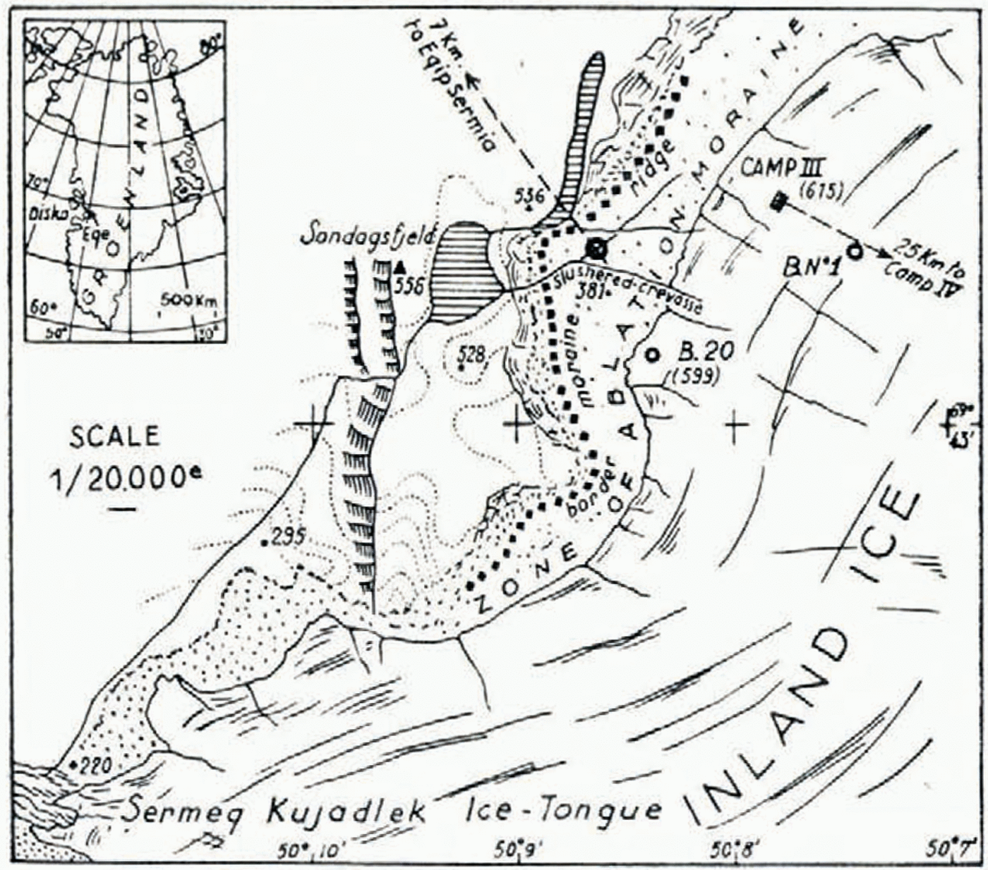
Fig.1 The border of the Inland Ice at Eqe, West Greenland

As the crevasse cut through the ablation moraine and was used as a channel for slush, the bottom was half filled with morainic boulders; so that rubbings could not be taken more than 2 m. below the surface.

Meteorological And Glaciological Data

We cannot give any accurate figures for the mean temperatures of air and ice at this spot throughout the year; the only available data on air temperatures are those in Bouché’s report.Reference Bouché ² At Camp III (alt. 615 m.), 600 m. east, observations from 14 July to 26 August gave a maximum of +7° C. and a minimum of –8.5° C., although temperatures of about –15° C. were occasionally recorded at the beginning of September. The mean annual temperature of the air is certainly below 0° C. since this is true even at the coast.

There are no local data on the mean temperature of the ice, but we know from several thermometric records from borings made during the 1449 and 1950 expeditions,Reference Cailleus ³ that the inland ice remains in overall thermal equilibrium with a slight negative vertical gradient instead of the positive gradient expected. In other words the inland ice is too cold for the present climate to a depth of at least 100 m. However, close to the ‘border of the cap, the ice seems to be less than 100 m. thick —at B.20 (Fig. 1), 400 m. south-east, it is 40–41 m. thick according to MartinReference Martin ⁴ —and it is therefore not at all certain that the vertical thermal gradient would be the same as further in.

The speed of ice flow was measured at the Ba beacon near Camp III; it was 0.10 m./day, to the south-west.Reference Nevière and Bauer ⁵ The total distance that this ice has flowed since precipitation cannot be computed with any certainty, because precipitation occurs over the whole ice cap; nor is it possible to know from what depth the measured crystals have come, because of the overthrusting and folding of the ice. The results of the geodetic. party in 1950Reference Nevière ⁶ shows that at Camp IV, 25 km. east-south-east of Camp III, the annual flow was 35 m., which gives the same mean velocity as that recorded at beacon B.1, so that this figure would seem to be typical of the ice edge.

Experimental Method

Four rubbings were taken, partly superposed on each other. After they had been photographed they were collected on a single drawing (Fig. 2, below), on which the crystals are numbered 1–77. In numbering we neglected partially recorded crystals; if such a crystal is large, like those marked E, F, the statistics might be altered by its omission, but in fact sufficient crystals are included to overcome this objection. Moreover, owing to melting, the paper quickly became soaked, and the outlines did not always appear satisfactorily, especially in the case of some smaller grains (see the top right of Fig. 2 between Nos. 13 and 69). The ratio between the number of large and small neglected crystals is much the same as for the measured crystals, so the results should not be seriously in error.

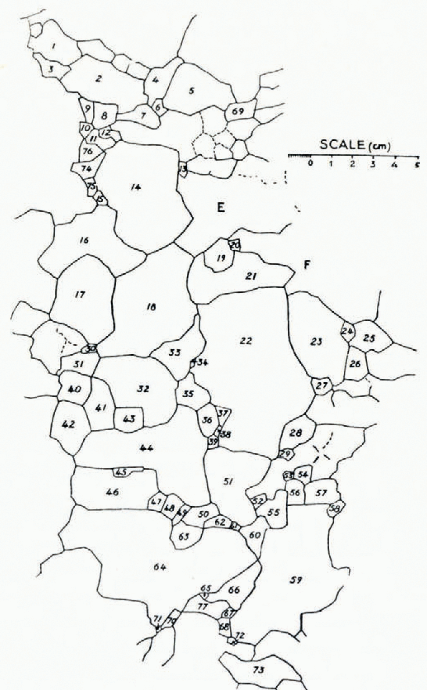
Fig. 2 The assemblage of the four rubbings; crystals numbered 1–77

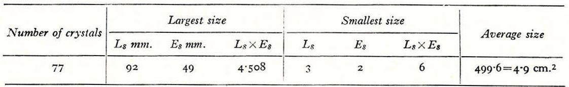
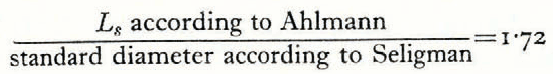
Areas were computed using Seligman’s method of comparison with standard circles of logarithmically increasing diameterReference Seligman ¹ ; and the root mean square diameter was calculated. We also calculated the average grain area by Ahlmann’s method,Reference Ahlmann ⁷ in which the longest dimension of each crystal’s section, L _s , is multiplied by the greatest breadth, E _s , measured perpendicular to the vector, L _s .

Results

The results obtained on Seligman’s method are summarized in Table I. The assemblage (Fig. 2) was referred to Mr. Seligman, who found 84 crystals as against our 77, and made the root mean square diameter 2.20 cm. as against our 2.16. This agreement shows that the method yields reasonably consistent results from one observer to another.

The results obtained using Ahlmann’s method are summarized in Table II.

TABLE I Grain size determined by Seligman’s method

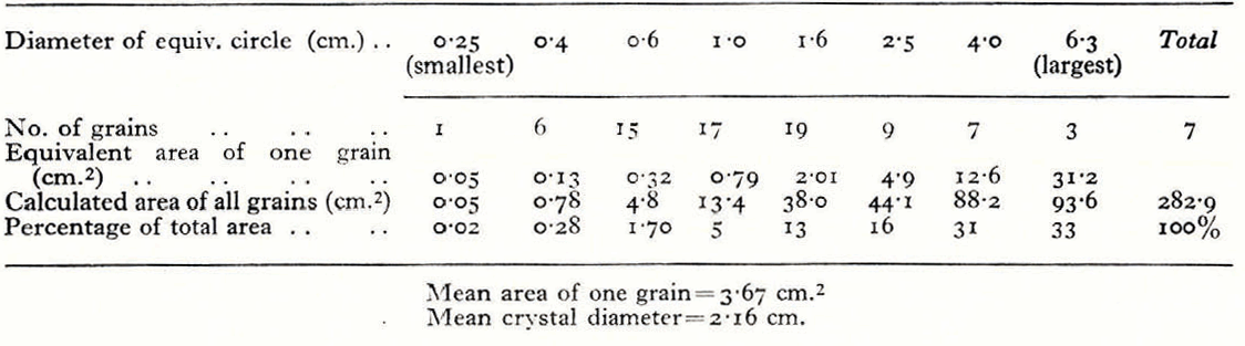
Table II Grain size determined by Ahlmam’s method

Discussion

The mean diameter (2.16 cm.) w area (4.9 cm.²) are close to those found by AhlmannReference Ahlmann ⁷ for the marginal stagnant ice of Isfallsglaciären in Swedish Lapland (2.4 cm. and 4.5 cm.). Similarly the mean diameter is within the range of values found by Seligman (2.05 to 2.34 cm.) at the snouts of various glaciers in the Swiss Alps which had a mean slope from bergschrund to snout of less than 10° (the Findelen Glacier, the Gorner Glacier and the two main streams of the Great Aletsch Glacier).

More data from other places are needed to know whether this agreement is a mere coincidence, or whether a diameter of 2 to 2.4 cm. is actually characteristic of the crystals at the end of a glacier, where melting can occur.

In order to compare the two methods, we have drawn granulometric curves (distribution curves of grain size), plotting diameter on a logarithmic scale against the cumulated area (Fig. 3, p. 327). Curve I was obtained by summing up the areas computed by Seligman’s method; this gave 8 points (▴) corresponding to percentages at the standard diameters. From the areas calculated using Ahlmann’s method, percentages were plotted against L _s dimensions. More points (Ο) are obtained by this method, but the calculation is more tedious.

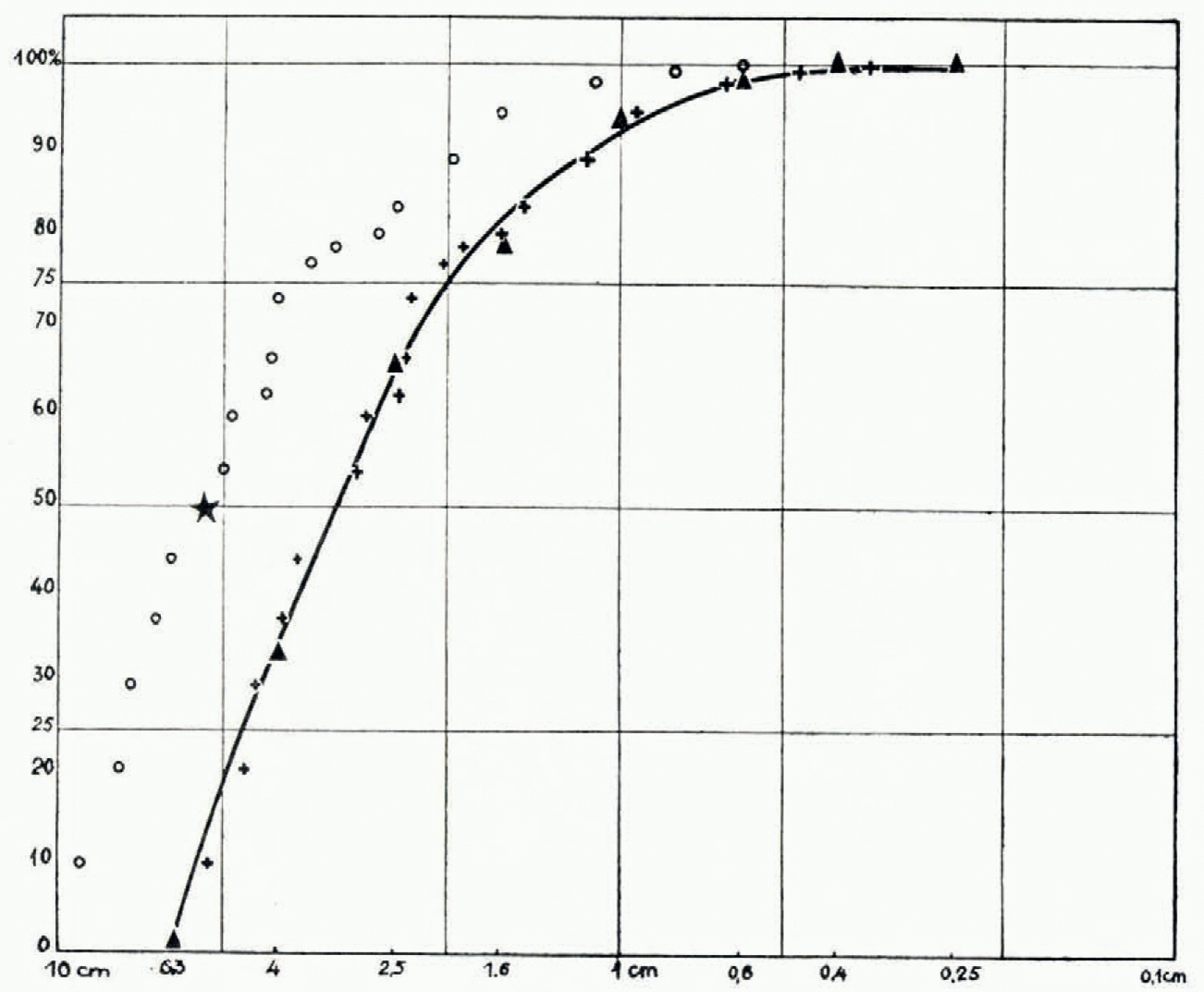
Fig. 3. (▲)—Curve I computed by Seligman’s method, (Ο)—Points computed by. Ahlmann’s method (+)—Points Ο translated by the distance needed to bring them onto Curve I

The two distributions are exactly similar. To verify this we moved all the points (Ο) to the right by the amount necessary to bring the “50% point” onto the Curve I. In this way we see that all the moved points (+) coincide with Curve I. The systematic space between the two curves means that:

()

This agreement emphasizes the value of Seligman’s method, for it is much quicker than Ahlmann’s method, and is just as accurate.

In order to compare the variation in size of the grains from an ice cap with the granulometric distribution of various detrital formations, the “indice d’hétérométrie” (heterometry index) was measured on Curve I by Cailleux’s method.Reference Cailleux ⁸

Using the statisticians’ “method of quartiles,” Cailleux has defined this index as the minimum value reached by the ratio

()

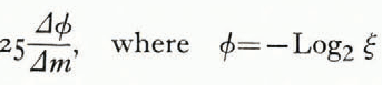
m is the cumulated mass (of pebbles, for instance) expressed as a percentage and plotted on ordinates (arithmetic scale) against the dimensions of grains, ξ, on abscissae (logarithmic scale). Consequently the scale of ϕ is arithmetic (Fig. 4, p. 329).

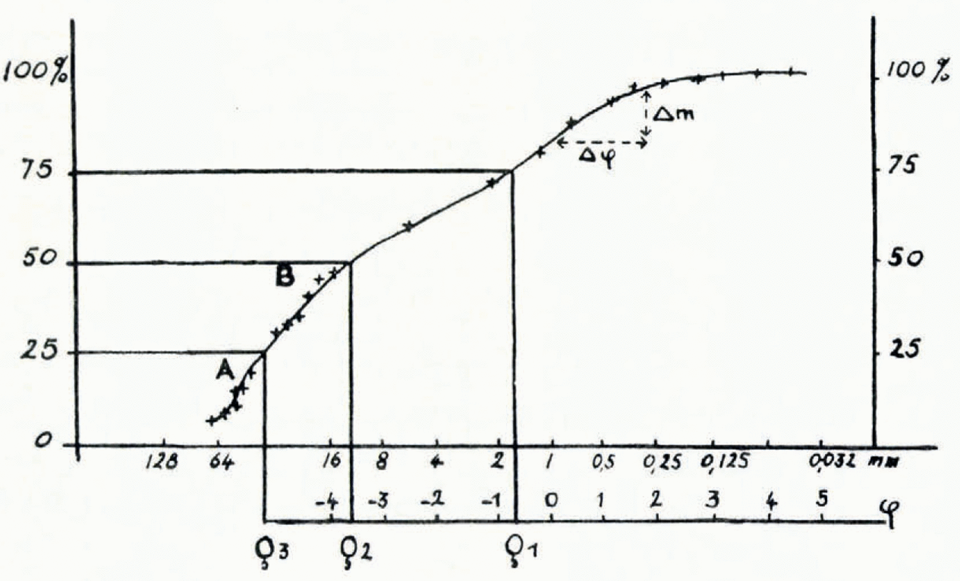
Fig. 4 Granulontetrie curve of quaternary alluvium from the River Marne near Champigny (Seine)—after Cailleux.Reference Cailleux ⁸ Abscissae show the dimension, ξ, of the pebbles and grains in mm., with a scale of ϕ below. Ordinates show the mass of pebbles and grains of dimensions larger than ξ as a percentage of the total mass. Q₂ is the median, Q₁ and Q₃ are quartiles. 25 is lowest between A and B.

Thus this index is the inverse of the slope of the steepest part of the curve corresponding to an interval of a quartile (Δm = 25%; so selected to avoid errors from defects in drawing the curve); see the example in Fig. 4. In other words, as Cailleux saysReference Cailleux ⁸ : “Dire que 25 est égal à 1,2,3 ou 4, revient à dire que la dimension des éléments [here, ice crystals] est divisée respectivement par 2, 4, 8 ou 16, lorsque, descendant l’échelle, on franchit un intervalle égal au quart (25%) de la masse totale de l’échantillon.” That is to say the heterometry index is small if grains are of similar size and large if they vary over wide limits.

On Curve I, m expresses the areas of crystals summed up in percentages; ξ, the standard diameters. The index is:

This value is rather low when compared with those found for detrital materials (pebbles, gravel or sand: from 0.2 to 3 or 4); so that crystallization seems to produce crystals of rather homogeneous dimensions. Indeed, as the dispersion in section is small, in volume it would be even smaller, because certain small areas on the section may be the cut of larger crystals. This may be evidence that melting accelerates the drainage of the liquid phase from the smallest crystals, which consequently melt faster as Seligman has suggestedReference Seligman ¹ leaving a higher percentage of larger crystals in the aggregate.

Melt water percolating through the interstices ought to wear away the crystal boundaries to a certain extent. To investigate this, we measured the “indices d’émoussé” (indices of smoothness) by Cailleux’s methodReference Cailleux ⁹ ; these are and where r ₁ is the smallest radius of curvature on the apparent outline, L the longest dimension of a crystal in section, and r ₂ the smallest radius, other than r ₁, of a point M such that between M and the point where r ₁ is found there is at least one point where the radius is R > r ₂ > r ₁. The “indices d’émoussé” were only measured on the longest crystals, because the uncertainty in the outlines of the smaller ones does not allow the computation of a radius of curvature.

Table III Indices of Smoothness of the Larger Crystals

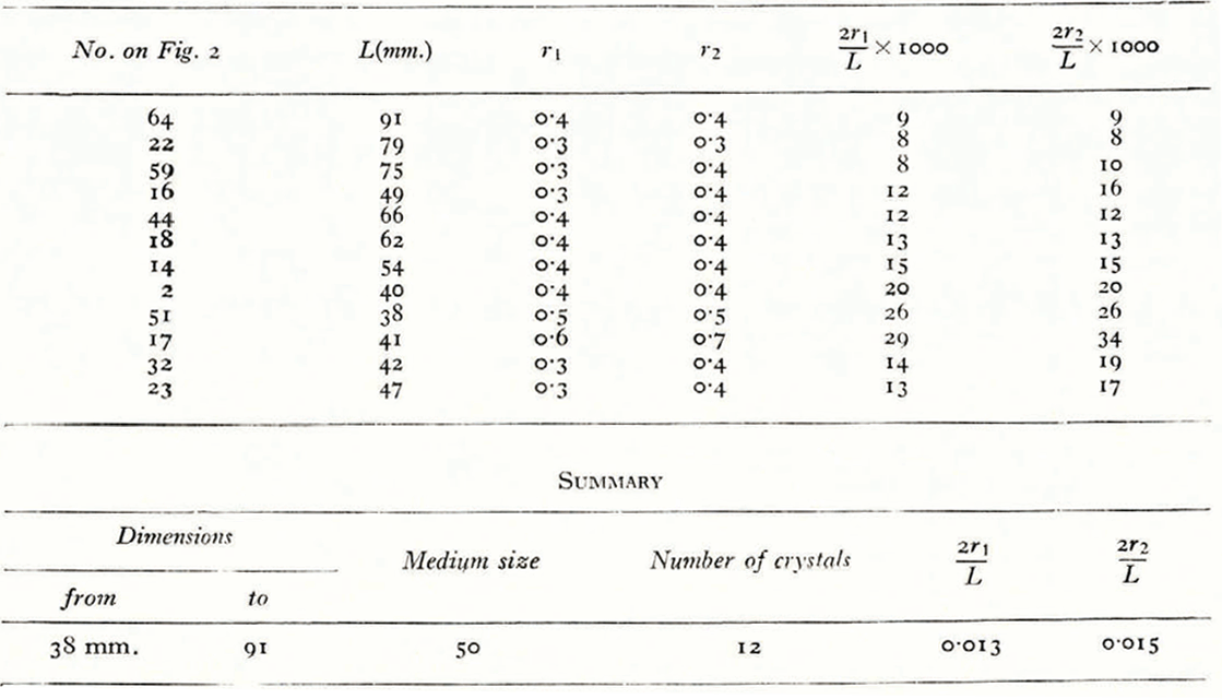
The indices of medium size, 0.13 and 0.015, are very low and have little significance, since they are near the errors of measurement. In other words, ice crystals show no noticeable erosion of their outline, but melt in thin films along their boundaries.

As it seems that large crystals do grow at the expense of small ones, rather than by the coalescence of several crystals of the same size, does the melt water play some other part?

SeligmanReference Seligman ¹ suggests that: “Thaw water, percolating in thin films through the interstices, will freeze on to the crystals when the temperature falls. The small crystals can thus thaw away and the large crystals grow.” But he adds the qualification “… at the few places where this ‘thaw-freeze’ can occur summer thaw will remove the whole glacier surface so affected.”

RenaudReference Renaud ¹⁰ presumes that the growth of glacier crystals depends essentially on their temperature, especially close to the melting point, because of the faster drainage of the saline water film off the interstices between two neighbouring crystals, which ought to make their coalescence easier. He adds: “L’orientation des cristaux et la pression jouent peut être un râle dans ce processus de croissance qui ale caractère d’une soudure autogène, sans modification dans l’équilibre thermique.”

These two hypotheses do not explain directly the low heterometry of the formation. It may be that there exist critical dimensions beyond which smaller crystals are absorbed in the growth of larger ones, as was first propounded by Hagenbach-Bischoff in his theory of 1888.Reference Hagenbach-Bischoff ¹¹

At all events, in active ice which is not flowing too fast and is at the melting point, the growth of ice crystals seems to tend to homogeneous crystal dimensions with a mean diameter of 2 to 2.4 cm.