


1. Introduction
In high-mountain environments glacial lakes are becoming increasingly common as a result of accelerating glacier mass loss. Their presence can pose significant outburst hazards, as well as impacting upon glacier mass balance and the local hydrological system (Reference Bajracharya, Shrestha and RajbhandariBajracharya and others, 2007; Reference RöhlRöhl, 2008; Reference McClymont, Roy, Hayashi, Bentley, Maurer and LangstonMcClymont and others, 2011). More recently concerns have also been raised as to their role in water availability issues (Reference Masetti, Diolaiuti, D'Agata and SmiragliaMasetti and others, 2009; Reference Langston, Bentley, Hayashi, McClymont and PidliseckyLangston and others, 2011). Moraine-dammed lakes can attain hazardous volumes over relatively short time frames, putting increasing strain on the often unconsolidated moraine dam (Reference Clague and EvansClague and Evans, 2000). At present, however, predicting where or when significant hazards will develop is not possible. Recent focus has been on reconstructing lake expansion from archival ground-based or aerial photographs (e.g. Reference Watanabe, Kameyama and SatoWatanabe and others, 1995) and on satellite imagery (e.g. Reference Allen, Owens and SirgueyAllen and others, 2008; Reference Bolch, Buchroithner, Peters, Baessler and BajracharyaBolch and others, 2008). Very little is known about subsurface structure or internal processes of the moraine dam, which are factors strongly influencing lake evolution and stability. Numerous processes have been identified as contributing to the degradation of terminal or lateral moraines (e.g. seepage erosion, and degradation of an ice-cored moraine dam (Reference Clague and EvansClague and Evans, 2000; Reference Richardson and ReynoldsRichard-son and Reynolds, 2000)). Often the cause is linked to a trigger, such as overtopping due to a surge wave caused by mass movement, which serves to compound a pre-existing weakness in the dam (Reference Korup and TweedKorup and Tweed, 2007). In addition, not all large moraine-dammed lakes pose significant hazards, because drainage can occur gradually if the level of the dam is reduced in a controlled manner over several years (e.g. Reference Hambrey, Quincey, Glasser, Reynolds, Richardson and ClemmensHambrey and others, 2008). A much better understanding of the internal moraine dam is required, therefore, to allow the prediction of potential hazards and to provide timely mitigation strategies.
Subsurface hydrological investigations have traditionally relied on coring and borehole-based surveys, but this can be expensive and logistically difficult in many glacial environments (e.g. Reference French, Binley, Kharkhordin, Kulessa, Krylov, Vereecken, Binley, Cassiani, Revil and TitovFrench and others, 2006; Reference McClymont, Roy, Hayashi, Bentley, Maurer and LangstonMcClymont and others, 2011). It is also widely accepted that the intrusive nature of such access-hole techniques can lead to artificial modifications of subsurface properties and processes, thus leading to biased observations. More recently, electrical geophysical techniques have been used with increasing frequency and success in both glacial and hydrological investigations (e.g. Reference Kulessa, Hubbard and BrownKulessa and others, 2003a, Reference Kulessa, Hubbard, Brown and Beckerb; Reference Rubin and HubbardRubin and Hubbard, 2005; Reference Vereecken, Binley, Cassiani, Revil and TitovVereecken and others, 2006; Reference KulessaKulessa, 2007; Reference Maurer and HauckMaurer and Hauck, 2007; Reference Kneisel, Hauck, Fortier and MoormanKneisel and others, 2008). Such techniques can provide cost-effective and minimally intrusive complements to more conventional access-hole surveys, facilitating the characterization of subsurface hydrological properties and processes beyond the point scale and thus extending spatial coverage.
In this paper, we report on integrated electrical resistivity tomography (ERT) and electric self-potential (SP) surveys carried out on a moraine complex adjacent to Miage glacier, Italy. These surveys allow assessment of coupled lake-dam hydrological processes that have important implications for moraine-dam stability. We conclude by discussing our results and techniques in the broader context of glacial-lake outburst prediction and mitigation.
2. Field Site And Lake History
Miage lake is located at ~2020 m a.s.l. on the southern lateral moraine of Miage glacier, Italian Alps (Fig. 1). The site was deemed to be an ideal location to develop and evaluate our methods as it is stable, easily accessible but provides an environment analogous to many more remote and challenging sites. Over the last 200 years, the lake has been characterized by a series of drainage and refilling episodes. Due to the high frequency of calving from the exposed ice face (Fig. 2a), the area has become a popular tourist attraction. The most recent drainage event occurred in 2004, when 80% of the lake's volume was lost in <72 hours, allowing direct observation of the lake-bed hydraulic system (Reference Deline, Diolaiuti, Mortara, Pavan, Smiraglia and TamburiniDeline and others, 2004). The lake is characterized by four main basins, contained within a series of breach-lobe moraines that are surficially connected through a number of altitudinal thresholds (Reference Masetti, Diolaiuti, D'Agata and SmiragliaMasetti and others, 2009). The first basin is in contact with an actively calving glacier ice face, and has an ice floor that in 2004 was inferred to extend some way through the central moraine complex (Reference Deline, Diolaiuti, Mortara, Pavan, Smiraglia and TamburiniDeline and others, 2004). This complex currently separates basin 1 from basins 2 and 3 (Fig. 2a and 3), which were found to be floored by glacial sediments (Reference Deline, Diolaiuti, Mortara, Pavan, Smiraglia and TamburiniDeline and others, 2004). Basin 4, to the west, is now well separated from the other three by moraine sediments (Fig. 3). Prior to 2004 all four basins were connected with each other to form one large lake, with an outflow located at the western end of basin 4. Following the drainage event in 2004, the lake, now three distinct water bodies, stabilized at a lower level. Currently only basins 2 and 3 are surficially connected (Figs 2a and 3). Reference Masetti, Diolaiuti, D'Agata and SmiragliaMasetti and others (2009) inferred the presence of a subterranean connection between basin 1 and basins 2 and 3, but no evidence was found of any connection with basin 4 (Fig. 3). This suggests that basins 1-3 are all predominantly glacier-fed, while basin 4 is hydraulically isolated from the system and supplied mainly by precipitation (Reference Masetti, Diolaiuti, D'Agata and SmiragliaMasetti and others, 2009). We therefore focus our attention on the area between basins 1 and 2 and basin 3, the location of the inferred hydrological connection (Figs 2a-c and 3). At present there are no visible outflows exiting at the lake perimeters.

Fig. 1. (a) The location of Miage glacier and glacial lake on the southern side of Mont Blanc, Italy. (b) Zoomed-in view of the glacial lake and surrounding topography (area shown within the rectangle in (a)).

Fig. 2. (a) Basins 1–3 of Miage glacial lake, August 2010. The main image shows the visual difference in water colour between basin 1 and basins 2 and 3. The visual difference was interpreted as a difference in suspended sediment content. The location of the SP reference electrode is shown on the moraine ridge above the study area. The dashed black arrows over the moraine complex depict the inferred hydrostatic potential from basin 1 to basins 2 and 3. (b) The change in lake level of each basin plotted against date (day/month). There are two measurements per day (am and pm) between 6 and 23 August 2011. (c) The change in lake level of basin 1 plotted against basins 2 and 3. The high correlation between the lake level changes during the investigation period in August 2010 is illustrated, with R 2 = 0.93.

Fig. 3. The ERT and SP surveys were co-located along eight profiles, with the addition of two SP grids, 2m × 2m, located at each end of the moraine complex. The locations of the reference electrode used in the measurement of the SP signal and the base station for the differential GPS measurements are also shown.
3. Methods
3.1. ERT and SP techniques
The theories and applications of ERT and SP techniques to subsurface hydrological problems are well established (e.g. Reference Rubin and HubbardRubin and Hubbard, 2005; Reference Vereecken, Binley, Cassiani, Revil and TitovVereecken and others, 2006). ERT surveys involve the measurement of the voltage difference between two electrodes, arising in the subsurface from the injection of a direct current using a separate electrode pair. By acquiring numerous such quadripole measurements using different electrode combinations and spacings, a multidimensional image of the bulk resistivity (or its inverse, bulk electrical conductivity) distribution in the subsurface can be constructed based on mathematical inversion. In most subsurface porous media, the transport of electrical current occurs predominantly via movement of ions in the pore fluid, so that a medium's electrical resistivity depends predominantly on fluid saturation, porosity and fluid electrical conductivity. Thus, ERT surveys can detect and delineate spatial or temporal changes in lithological or hydrological properties of glacial sediments (e.g. Reference KulessaKulessa and others, 2007; Reference Hiemstra, Kulessa, King and NtarlagiannisHiemstra and others, 2011; and references therein).
SP surveys exploit the presence of naturally occurring electrical potentials in the subsurface. At the Miage moraine/lake complex we have no reason to expect the presence of significant thermal or chemical gradients, or of significant microbial activity. In this situation, and in the absence of artificially injected currents, we expect streaming currents to be the dominant SP source. Natural pore waters generally have an excess of electrical charge, ![]() , due to the existence of an electrical double layer at the surface of the sediment grains. The charge density, Q
v, is
, due to the existence of an electrical double layer at the surface of the sediment grains. The charge density, Q
v, is
where q
i
is the charge of ionic species i, and ![]() is the average concentration of ionic species i (Reference Revil, Linde, Cerepi, Jougnot, Matthäi and FinsterleRevil and others, 2007). The sign of Q
v therefore depends on the types of ionic species present, as well as their relative charges and concentrations. It can be shown that (e.g. B. Kulessa and others, unpublished information)
is the average concentration of ionic species i (Reference Revil, Linde, Cerepi, Jougnot, Matthäi and FinsterleRevil and others, 2007). The sign of Q
v therefore depends on the types of ionic species present, as well as their relative charges and concentrations. It can be shown that (e.g. B. Kulessa and others, unpublished information)
where ε is the pore-fluid dielectric constant, ζ is the zeta potential, k is permeability, F is the formation factor and S
w is fluid saturation. In most glacial sedimentary settings, ζ and therefore Q
v can be expected to be negative (as all other parameters are positive); however, it is possible for ζ to be positive, for instance in fresh snow samples (e.g. B. Kulessa and others, unpublished information). The advective drag of the excess of electrical charge is responsible for streaming currents with density j
s, whose divergence and curl generates a quasi-static electromagnetic field known as the streaming potential (Reference SillSill, 1983; Reference Revil, Schwaeger, Cathles and ManhardtRevil and others, 1999a,b). In fully saturated media the source current density, j
s, is related to the excess of charge, ![]() by
by
where u is the Darcy velocity (Reference Revil, Linde, Cerepi, Jougnot, Matthäi and FinsterleRevil and others, 2007). As a consequence, SP measurements made at the ground surface can be sensitive indicators of subsurface water flux through the dependency on u, and of the properties of the fluid and fluid/matrix interface through the dependency on the excess of charge, ![]() (Reference SillSill, 1983; Reference Darnet, Marquis and SailhacDarnet and others, 2003; Reference Revil, Titov, Doussan, Lapenna, Vereeck-en, Binley, Cassiani, Revil and TitovRevil and others, 2006; Reference JardaniJardani and others, 2007; Reference Sheffer and OldenburgSheffer and Oldenburg, 2007; Reference Moore, Bolève, Sanders and GlaserMoore and others, 2011). Since the decay of streaming-potential amplitudes is a function of depth, SP measurements made at the ground surface can also be used to delineate phreatic surfaces (e.g. Reference FournierFournier, 1989; Reference BirchBirch, 1993; Reference Revil, Naudet, Nouzaret and PesselRevil and others, 2003; Reference LindeLinde and others, 2007; Reference JardaniJardani and others, 2009). Specifically, as a result of the depth dependency, topographic highs and lows are normally associated with positive and negative SP anomalies respectively (Reference Revil, Naudet, Nouzaret and PesselRevil and others, 2003). The SP technique has so far seen surprisingly little application in glacial environments (Reference Blake and ClarkeBlake and Clarke, 1999; Reference Kulessa, Hubbard and BrownKulessa and others, 2003a,b; Reference KulessaKulessa, 2007).
(Reference SillSill, 1983; Reference Darnet, Marquis and SailhacDarnet and others, 2003; Reference Revil, Titov, Doussan, Lapenna, Vereeck-en, Binley, Cassiani, Revil and TitovRevil and others, 2006; Reference JardaniJardani and others, 2007; Reference Sheffer and OldenburgSheffer and Oldenburg, 2007; Reference Moore, Bolève, Sanders and GlaserMoore and others, 2011). Since the decay of streaming-potential amplitudes is a function of depth, SP measurements made at the ground surface can also be used to delineate phreatic surfaces (e.g. Reference FournierFournier, 1989; Reference BirchBirch, 1993; Reference Revil, Naudet, Nouzaret and PesselRevil and others, 2003; Reference LindeLinde and others, 2007; Reference JardaniJardani and others, 2009). Specifically, as a result of the depth dependency, topographic highs and lows are normally associated with positive and negative SP anomalies respectively (Reference Revil, Naudet, Nouzaret and PesselRevil and others, 2003). The SP technique has so far seen surprisingly little application in glacial environments (Reference Blake and ClarkeBlake and Clarke, 1999; Reference Kulessa, Hubbard and BrownKulessa and others, 2003a,b; Reference KulessaKulessa, 2007).
3.2. ERT data acquisition and processing
We acquired eight ERT profiles using an IRIS Syscal-Pro 24-node imaging system with stainless-steel electrodes. The standard Wenner acquisition geometry was used, characterized by equally spaced electrodes arranged in a straight line. This geometry has been shown to yield stable results in resistive heterogeneous settings such as ours (e.g. Reference Kneisel, Hauck, Fortier and MoormanKneisel and others, 2008). We varied the electrode spacing between a maximum of 5 m for deeper-penetration surveys with a coarser resolution, and a minimum of 1 m for spatially highly resolved surveys with a reduced depth penetration (Fig. 3). The three-dimensional (3-D) position of each electrode location along all eight profiles was measured using a Leica Geosystems 1200 differential GPS. The GPS data were post-processed relative to a base station located in a fixed position on the central moraine complex (Fig. 3). The nominal accuracy of the post-processed GPS data is ±1 cm in the horizontal and ±2 cm in the vertical.
Following Reference Binley, Ramirez, Daily, Beck, Hoyle, Morris, Waterfall and WilliamsBinley and others (1995), we expect systematic acquisition errors to arise from poor electrode contact, as well as random errors to be introduced by the measurement device or non-deterministic external effects. To minimize electrode-contact errors and the impact of any external influences, ERT data acquisition adopted the procedures identified by Reference Hauck, Isaksen, Vonder Mühll and SollidHauck and others (2004) and Reference Kneisel, Hauck, Fortier and MoormanKneisel and others (2008). Locations that lacked clay-like surface materials were additionally irrigated with a salt-water solution. Where this was not possible, salt-water saturated sponges were wrapped around the electrodes, held in place by rubber bands, and wedged between rocks on the moraine surface (Reference Maurer and HauckMaurer and Hauck, 2007). To quantify acquisition errors,
-
several repeat measurements using any single quadripole were acquired and stacked, yielding an average resistance datum and a diagnostic standard deviation. Any resistance datum with a standard deviation greater than 3% (after Reference Langston, Bentley, Hayashi, McClymont and PidliseckyLangston and others, 2011) was discarded.
-
any single quadripole measurement and its repeats were replicated with swapped current and voltage electrodes, to yield reciprocal data for each ERT profile. Reciprocity is a better indicator of error than repeatability (Reference Binley, Ramirez, Daily, Beck, Hoyle, Morris, Waterfall and WilliamsBinley and others, 1995). We found very high correlations between our direct and reciprocal measurements (r = 0.998) for the entire dataset (Fig. 4a). Reciprocal errors were calculated as a percentage of resistance, and any reciprocal error greater than 5% was discarded. Only eight data points were removed from our entire dataset, all located in profile 7. It is probable that this was due to the numerous large boulders (with associated air spaces) located along this profile.
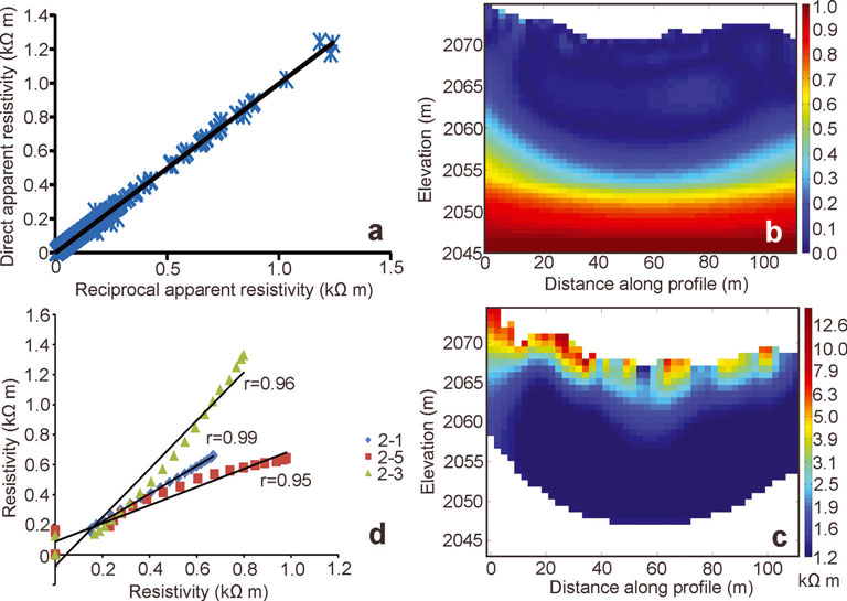
Fig. 4. (a) Direct resistivity values plotted against their relative reciprocal resistivity values for all eight profiles. A significant correlation (r = 0.998) exists between the two measurements. (b) The DOI index for ERT profile 2. (c) Final inversion values of ERT profile 2 plotted against the values of profiles 1, 3 and 5 at points where they intersect. (d) The final inversion results for ERT profile 2; all data with a corresponding DOI index of >0.2 have been removed.
All resistivity data were inverted using the finite-difference code DCIP2D, made available by the Geophysical Inversion Facility of the University of British Columbia, Canada (e.g. Reference Oldenburg and LiOldenburg and Li, 1994; Reference Li and OldenburgLi and Oldenburg, 2000). The model is a finite-difference mesh, divided into rectangular cells which define an area of interest, and padding cells on three sides to ensure the correct boundary conditions can be applied. The code minimizes a discretized version of the model objective function, ϕm (e.g. Reference Oldenburg and LiOldenburg and Li, 1994):

where m and m 0 are the current and reference models respectively. The constant α s (damping factor) controls the closeness between the current model and the reference model, while the constants αx and αz control the model roughness in the horizontal and vertical directions respectively. Minimization is achieved iteratively by updating m with respect to m 0 based on the misfit functional, ϕd:
where ![]() and d
pred are the measured and computed data respectively, and εi, are the measurement errors.
and d
pred are the measured and computed data respectively, and εi, are the measurement errors.
An average of seven iterations was required to produce final inverted ERT models that fit the data to within a 5% root-mean-square (RMS) error level. We performed two main reliability checks to identify and eliminate artefacts produced by the mathematical reconstruction. First, we adopted the concept of the depth of investigation (DOI) index (e.g. Reference Oldenburg and LiOldenburg and Li, 1999; Reference Hilbich, Marescot, Hauck, Loke and MäusbacherHilbich and others, 2009). This index requires two inversions to be carried out for each profile, using alternating reference models set to values of one-tenth and ten times the average apparent resistivity measured for that profile. An increase in damping factor to αs = 0.05 is used to ensure closeness between the reference and iteratively updated current models. The DOI index is then calculated from
where m 1(x,z) and m 2(x,z) are the resistivity values in the two final models, and m 01 and m 02 are the values of the corresponding reference models. R b are the resistivity values at the bottom of the two final models, expected to be equal to or at least very close to the corresponding value of the reference model. In practice, this value is used in the normalization of the DOI index. In areas where the final models are well constrained by the data, and the inversion process therefore considered reliable, the DOI index is close to zero (Fig. 4b). Any cells with a DOI index greater than 0.2 (after Reference Oldenburg and LiOldenburg and Li, 1999; Reference Hilbich, Marescot, Hauck, Loke and MäusbacherHilbich and others, 2009) were considered less reliable and thus rejected (Fig. 4c). Second, we plotted against each other the inverted final resistivity values along the one-dimensional intersection between any two of our ERT profiles (Fig. 3). This was done after application of the DOI index concept, so that the final resistivity values of any two intersecting ERT profiles could be expected to be near-identical if the inversion process was reliable. Indeed, in all cases we obtained correlation coefficients greater than 0.94 (Fig. 4d), confirming the reliability of our final ERT models.
3.3. Acquisition and processing of SP data
SP surveys were carried out at 1m intervals along all eight ERT profiles, with the addition of two 2m × 2m grid-based SP surveys (Fig. 3), generating a total of 525 individual measurements. We used commercially available, non-polarizing lead/lead-chloride (‘Petiau’) electrodes (Reference PetiauPetiau, 2000), together with an Agilent Technologies U1251A high-impedance multimeter. At each measurement point, a saltwater- soaked sponge was also wrapped around the roving electrode’s contact area to minimize the contact resistance. All SP data were collected relative to the same reference electrode, located on the moraine ridge to the east of the surveyed moraine complex, at an elevation of 2085.3ma.s.l., roughly 25 m above the lake water level and >10 m higher than the highest point in the survey area (Figs 2 and 3). At this location, temporal variations in streaming potentials were expected to be negligible due to the lack of surface recharge in the form of precipitation (or snowmelt) during the study period. Any minor temporal variations in subsurface streaming potentials can be accounted for in the drift correction (below). A salt-water soaked sponge was wrapped around the reference electrode's contact area, and 'watered' regularly throughout each survey day to prevent it drying out. In a remote location such as our field site, we can expect cumulative electrode drift to occur due to time-dependent telluric currents caused by variations in the Earth's magnetic field, as well as relatively minor drift caused possibly by electromagnetic radiation emitted by cultural sources, including power lines, factories, radio communications and even fences (Reference Corry, De Moully and GeretyCorry and others, 1983), or temporal variations in streaming potentials at the reference electrode (Reference Corwin and WardCorwin, 1990). Cumulative drift was therefore recorded by repeatedly measuring several common tie-in points throughout the data collection, including tie-in points immediately adjacent to the reference electrode to check electrical stability. The raw SP data were then drift-corrected using standard procedures (e.g. Reference Naudet, Revil, Rizzo, Bottero and BègassatNaudet and others, 2004; Reference Doherty, Kulessa, Ferguson, Larkin, Kulakov and KalinDoherty and others, 2010). The location of every SP measurement station was surveyed in three dimensions by differential GPS using the same methods and base station location as for the ERT surveys (Fig. 3).
4. Results
The visible suspended-sediment concentration is markedly higher in lake basin 1 than in basins 2 and 3 (Fig. 2a). Manual monitoring of lake levels throughout the 3 week study period revealed a linear relationship (R2 = 0.93) of lake level change between the two water bodies, with a diagnostic lag in the change of basins 2 and 3 relative to that of basin 1 (Fig. 2b and c). Assuming that lake recharge occurs primarily through meltwater delivery in basin 1, this observation implies the presence of an efficient subterranean hydraulic link between upflow basin 1 and downflow basins 2 and 3 (Fig. 2a).
All eight ERT profiles were consistently characterized by a dominant two-layer structure (Fig. 5a). A more resistive upper layer of >4 kΩ m overlies a less resistive lower layer of <1 kΩ m-1 (Fig. 5b). The undulations of the interface between these two layers track the surface topography (Fig. 5a). Typically the upper layer is 5-10 m thick, and the lower layer extends to the depth limit of the ERT data according to the DOI index. There is some local variability in the resistance of the upper layers, with values ranging from 4 to 12.5 kΩ m, but the lower, less resistant layer is by contrast consistent (~1 kΩ m).

Fig. 5. (a) Inverted ERT profiles for all eight two-dimensional survey lines plotted in a 3-D grid. The distinctive two-layer pattern is visible across all profiles. (b) Resistivity values down a column of ERT profile 2, indicated by the dashed line in (a). The transition from the high-resistivity layer down to the low-resistivity layer at depth is illustrated.
The drift-corrected SP data are characterized by a spatially non-uniform distribution over the moraine-dam complex (Fig. 6a), varying in amplitude within the approximate range -30 to +70 mV. The individual data points were interpolated to form a continuous SP signal over the moraine complex using the ArcGIS topo to raster tool (Fig. 6a). This method uses an iterative finite-difference technique that is optimized to have the computational efficiency of local interpolation methods (e.g. inverse distance weighted (IDW) interpolation) without losing the surface continuity of global interpolation methods (e.g. kriging and spline) (Reference Hutchinson and DowlingHutchinson and Dowling, 1991). Within the central moraine-dam complex we observe a tendency for higher and lower SP values to occur at higher and lower moraine elevations respectively. The topographic high in the west of the moraine-dam complex is characterized by markedly negative SP values, and thus presents a notable exception to that pattern (Fig. 6a and b). Notwithstanding, we can infer that surface topography appears as a control on the drift-corrected SP data.
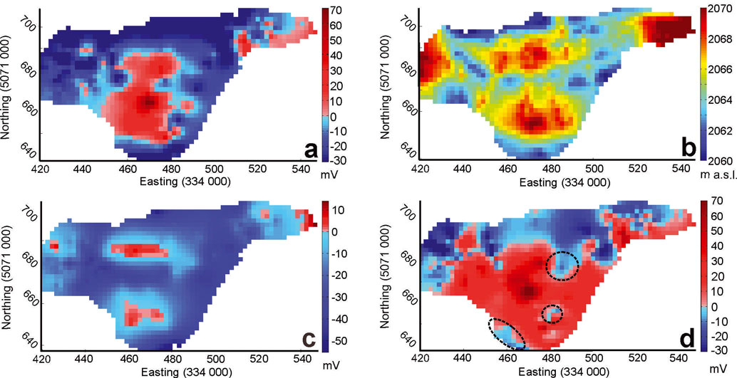
Fig. 6. (a) The drift-corrected SP signal, interpolated over the central moraine complex. Overall the higher positive-signal anomalies are found in higher-elevation areas and the low signal anomalies in the low-elevation areas around the lake perimeters (see (b)). (b) Elevation of the central moraine complex. Created from >7000 GPS points taken during the field season (points with an elevation standard deviation of >5% were removed) and interpolated as in the SP interpolations (see Section 4). (c) The topography-related bias for the study area, calculated from the estimated values of K and φ0(d) The topography-corrected map of electrical streaming potentials across the study area. Lower negative SP signals are found towards the basin 1 side of the moraine complex, close to the perimeter, with higher positive SP values located in the half towards basins 2 and 3, implying flow from basin 1 to basins 2 and 3. The circled regions highlight spatial non-uniformity, areas of negative polarity closer to basins 2 and 3.
5. Interpretation
5.1. ERT data
Glacier ice has a resistivity of ≫104kΩm in cold ice-sheet settings, and several magnitudes larger than that in warmer alpine settings (Reference KulessaKulessa, 2007). The lower layer delineated by our ERT surveys, which would previously have contained the ice-bed extension of lake basin 1 (Reference Deline, Diolaiuti, Mortara, Pavan, Smiraglia and TamburiniDeline and others, 2004), is characterized by resistivities of <1 kΩ m (Fig. 5a). In light of this, we can confirm that the ice bed of basin 1 no longer extends into the moraine complex. Since the last lake drainage in 2004, any remaining ice in the moraine complex has therefore melted out, consolidating the morainic material.
The resistivity values characterizing the upper (>4kΩ m; Fig. 5a) and lower (<1 kΩ m; Fig. 5a) layers in this complex are entirely consistent with those expected for unsaturated and saturated morainic material (Reference ReynoldsReynolds, 1997, p.422). The undulating interface between the unsaturated and saturated layers, at an approximate depth of 5-10 m, is spatially continuous across the entire moraine complex (Fig. 5a). The undulations of this interface mimic the ground-surface relief, but are generally smoother and less pronounced (Fig. 5a). As such they are consistent with the free surface of an unconfined groundwater aquifer that tracks the surface topography as a result of capillary forces (Reference FittsFitts, 2002). In Section 4 we inferred the presence of an efficient hydraulic link through the moraine complex, allowing the downstream basins 2 and 3 to respond rapidly to any glacier-melt-derived recharge of the upstream basin 1 (Fig. 2a). Thus the saturated layer within the moraine complex connecting these basins is likely subject to discharge, again akin to a groundwater aquifer. The local variability found in the upper, more resistive layer is likely to be a result of the structural heterogeneity of the moraine surface; however, we cannot interpret this at a fine scale due to the lack of detailed ground-truthing.
5.2. SP sources and topographic bias
We can expect to measure electrical streaming potentials generated by the water discharge in the saturated layer. Lateral variations in the bulk resistivity of this layer across our survey area are small (Fig. 5a), consistent with limited variability in its bulk sedimentological characteristics and pore-water electrical properties. We can therefore assume that lateral variations in the bulk distribution of the excess of charge, ![]() , within the saturated layer are equally limited, so that our measured SP data will have a strong association with the Darcy velocity, u, of flow in this layer (Eqn (3)). However, the decay of the streaming potentials between the free surface and the ground surface will be subject to noticeable topographic bias, since the free surface represents a smoother image of the considerable surface relief within our study area (see Section 3.1). The observed tendency for higher and lower SP values to occur at higher and lower moraine elevations respectively (Fig. 6a and b) is therefore unsurprising. Although the reconstruction of the location and undulations of the free surface from surface SP measurements is interesting in its own right (Section 3.1), we are primarily concerned with inter-basin water movement, which will indicate a glacial hazard potential. Thus, for the present purposes we choose to correct our SP data to remove the topographic effect to reveal associations between streaming potentials and inter-basin water discharge.
, within the saturated layer are equally limited, so that our measured SP data will have a strong association with the Darcy velocity, u, of flow in this layer (Eqn (3)). However, the decay of the streaming potentials between the free surface and the ground surface will be subject to noticeable topographic bias, since the free surface represents a smoother image of the considerable surface relief within our study area (see Section 3.1). The observed tendency for higher and lower SP values to occur at higher and lower moraine elevations respectively (Fig. 6a and b) is therefore unsurprising. Although the reconstruction of the location and undulations of the free surface from surface SP measurements is interesting in its own right (Section 3.1), we are primarily concerned with inter-basin water movement, which will indicate a glacial hazard potential. Thus, for the present purposes we choose to correct our SP data to remove the topographic effect to reveal associations between streaming potentials and inter-basin water discharge.
Following Reference FournierFournier (1989), Reference Revil, Naudet, Nouzaret and PesselRevil and others (2003) proposed that the free surface carries a dipolar charge with strength proportional to the hydraulic head in the saturated layer, as described by the water table model:
where h(x,y) and h0(x,y) are the elevations of the free surface at the measurement and reference electrodes, ϕ(x, y, z) and φ0(x, y, z) are the electrical potentials at these two electrodes respectively, and C sat and C unsat are the electrokinetic coupling coefficients in the saturated and unsaturated zones. The generalized macroscopic electro-kinetic coupling coefficient, C, is given by the Helmoltz-Smoluchowski equation (e.g. Reference Dukhin, Derjaguin and MatijevicDukhin and Derjaguin, 1974):
where εf, σf and ηf are the dielectric constant, the electrical conductivity and the dynamic viscosity of the pore fluid, and ζ is the zeta potential that characterizes the electrical potential of the double layer at the fluid/matrix interface (Reference Revil, Schwaeger, Cathles and ManhardtRevil and others, 1999b). The bulk electrical resistivity of the geological medium, ρb, is given by ρb = σf -1 F where F is the electrical formation factor. From a practical perspective, spatial changes in SP signal amplitude, φ(P), relative to reference potential, ϕ 0, can be related to corresponding variations in free-surface depth, where e is the elevation of the point of observation (above datum) and h is the elevation of the water table (above datum); thus e-h represents the thickness of the vadose zone below a measurement point P, and
where K is closely related to the electrokinetic coupling coefficient (in Reference Revil, Naudet, Nouzaret and PesselRevil and others (2003), K ≈ C/4). This semi- empirical relationship thus implies that K and φ0 can be estimated from a plot of measured SP data against (e-h). The underlying assumptions are that spatial variations in (1) the excess of charge, ![]() (Eqn (3)), and thus also K; (2) the Darcy velocity, u; and (3) the bulk resistivity of the unsaturated layer, are small enough so that linearity applies. We adopt a two-stage strategy in correcting our measured SP data for the topographic effect using Eqn (9). First we demonstrate that our SP profile 2 (Fig. 3) meets all of the above three assumptions which underlie Eqns (7-9). Application of Eqn (9) to that profile thus allows the unknown parameters K and ϕ
0 to be estimated, effectively calibrating the relationship between φ(P) and (e- h). Second, we can now use Eqn (9) to calculate the topography effect for the whole of our study area, and subsequently correct our measured SP data by subtraction of this calculated topographic effect. The correction procedure makes the further assumption that any spatial variations of the estimated values of K and φ
0 across our study area are insignificant.
(Eqn (3)), and thus also K; (2) the Darcy velocity, u; and (3) the bulk resistivity of the unsaturated layer, are small enough so that linearity applies. We adopt a two-stage strategy in correcting our measured SP data for the topographic effect using Eqn (9). First we demonstrate that our SP profile 2 (Fig. 3) meets all of the above three assumptions which underlie Eqns (7-9). Application of Eqn (9) to that profile thus allows the unknown parameters K and ϕ
0 to be estimated, effectively calibrating the relationship between φ(P) and (e- h). Second, we can now use Eqn (9) to calculate the topography effect for the whole of our study area, and subsequently correct our measured SP data by subtraction of this calculated topographic effect. The correction procedure makes the further assumption that any spatial variations of the estimated values of K and φ
0 across our study area are insignificant.
Based on the consistent measured/modelled resistivity values of the saturated layer, we infer that variations of Q v (and thus also of K) within our study area are likely limited, so that assumption 1 is met. Although we cannot exclude spatial variations in the Darcy flux across the moraine complex from basin 1 in the direction of basins 2 and 3 (Figs 2 and 3), the variations orthogonal to this are likely to be negligible across the length of the moraine. The governing equations of streaming potentials generated by orthogonal flow regimes are linearly independent (Reference Kulessa, Hubbard and BrownKulessa and others, 2003a). We can therefore assume that the magnitude of streaming potentials generated along the length of the moraine, and certainly the magnitude of spatial variations in such potentials in that direction, are also negligible. Thus, assumption 2 is met for our SP profiles 1 and 2 that were acquired along the length of the moraine (Fig. 3). We had ascertained above that lateral variations in the bulk resistivity of the saturated layer are likely small enough to be ignored. Unfortunately this is not the case for the unsaturated layer, which is subject to bulk resistivity variations of up to approximately one order of magnitude (Fig. 5a). Any change in the bulk resistivity of this layer will affect the value of K as described by Eqn (9), and thus also affect streaming potentials measured at the ground surface as described by Eqns (6) and (7). As a consequence of the significant expected variations of K, it is not surprising that the application of Eqn (9) to our SP data was dominated by nonlinearity in the slope K(e-h). Only in the case of SP profile 2 did we obtain a statistically significant (R2 = 0.69) straight-line fit between φ(P) and (e-h) (Fig. 7). This finding is readily expected since SP profile 2 is orientated most orthogonally to the expected dominant direction of subsurface water seepage (i.e. from basin 1 to basin 2; Fig. 3). The streaming-potential contribution to the total measured SP data for profile 2 is in this case very small, as dictated by the principle of linear independence (see above; Reference Kulessa, Hubbard and BrownKulessa and others, 2003a,b), so the SP signal generated by the topographic effect dominates along profile 2. In contrast, for all other SP profiles the total measured SP signal is a combination of the topography effect and a streaming-potential contribution, implying that we will not be able to obtain a straight-line fit by applying Eqn (9) to these profiles. Recognizing the residual uncertainty, we may thus conclude that any effects of lateral changes (along the length of the moraine) in the bulk resistivity of the unsaturated layer on the measured SP data in profile 2 are small. Using the estimated values of K (6.18) and φ 0 (-70.8) from profile 2, we can calculate the therefore topographic effect for the whole of our study area (Fig. 6c), and subsequently subtract it from the measured SP data (Fig. 6a). This yields a topography-corrected map of residual electrical streaming potentials across our study area (Fig. 6d).

Fig. 7. φ(P) plotted against (e–h) for SP profile 2. A significant linear relationship exists between the two variables, R 2 = 0.69.
5.3. Inferred streaming-potential map
The residual streaming-potential map (Fig. 6d) is characterized by a negative to positive gradient exceeding 100 mV, from <-30 mV to ≫+70 mV across the central moraine complex from basin 1 towards basins 2 and 3 (Figs 2 and 3). These inferred changes in residual streaming-potential magnitude and electrical polarity are entirely consistent with those typically observed for water seepage through earth dams (Reference Bolève, Revil, Janod, Mattiuzzo and FryBolève and others, 2009 and references therein). This inference suggests that contemporary moraine dams are characterized by similar streaming-potential properties and processes to earth dams in non-glacial settings. In the present case, the residual streaming-potential map (Fig. 6d) is thus consistent with water seepage from basin 1 to basins 2 and 3, as indeed expected from our lake- level observations (Section 4; Fig. 2). The inferred pattern of residual streaming-potential change is spatially non-uniform, as there is not a graduated pattern of high positive to high negative values in the direction of basins 2 and 3 along the length of the moraine. Some regions of negative polarity appear closer to basin 2 relative to the surrounding areas of positive polarity (Fig. 6d). Such non-uniformity may indicate spatial variability in subsurface water-flow patterns, which could intuitively be expected given the complex geometrical arrangement of the central moraine complex (Figs 2 and 3). However, aerial coverage of our data is too sparse to allow reliable conclusions to be drawn without over-interpretation of the map and a more robust calculation of uncertainties. We made several assumptions in deriving the residual streaming-potential map that are difficult to quantify, and that constrain any such interpretation. These include small or negligible changes in moraine sedimentological compositions or architectures, pore-fluid electrical properties and saturated and unsaturated layer bulk resistivities.
6. Conclusions
ERT and SP surveys were carried out on the central moraine complex of Miage glacial lake. A total of eight ERT profiles and >500 SP measurement stations, in a range of profiles and grids, were acquired. The inverted ERT data are spatially consistent throughout our study area, are characterized by a higher-resistivity layer (≫4kΩ m) overlying a layer of markedly lower resistivity (<1 kΩ m) (Fig. 5a) and are interpreted as unsaturated and saturated morainic materials respectively. Areas of buried ice are not detected by our data, suggesting that any such ice present in the past (Reference Masetti, Diolaiuti, D'Agata and SmiragliaMasetti and others, 2009) has now melted out. The morphology of the interface between these two layers represents a smoothed reproduction of the ground-surface relief, and as such is strongly reminiscent of the free surface of an unconfined groundwater aquifer.
The measured SP data were corrected for topographic effect, introduced by variable thicknesses of the unsaturated layer across our survey area, using pertinent theory of electrography. The residual streaming-potential map (Fig. 6d) reflects bulk subsurface water seepage from the ice-proximal basin 1 to the more distant basins 2 and 3 (Figs 2 and 3), and in terms of streaming-potential magnitude and upstream/downstream polarity change (from <-30 to ≫+70 mV) is consistent with water seepage through earth dams in various non-glacial settings (Reference Bolève, Revil, Janod, Mattiuzzo and FryBolève and others, 2009). Our findings thus confirm earlier work by Reference Masetti, Diolaiuti, D'Agata and SmiragliaMasetti and others (2009) based on geological mapping and tracer tests, as well as our own lake-level observations (Fig. 2) that were consistent with an efficient hydraulic link between the two basins. We made several assumptions in deriving the streaming-potential map, including those of small or negligible differences in, for example, moraine sedimentological compositions or architectures, pore-fluid electrical properties and saturated and unsaturated layer bulk resistivities.
Our findings have significant implications for investigating the stability and hazard potential of moraine dams. Not only are the methods largely non-intrusive and inexpensive, but they have proved effective in characterizing the subsurface hydrogeological setting in a notoriously heterogeneous glacial moraine-dam setting. Variable subsurface water saturation and flow are both factors that contribute significantly to areas of potential weakness and degradation in non-ice-cored moraine dams. A combination of these methods provides a significantly improved methodology for investigating the potential for catastrophic lake outburst from moraine-dammed lakes. The cost-effective and highly portable nature of the techniques provides scope for much-needed research in many mountainous regions where access may be difficult but lake drainage can have severe impacts on safety and the fragile mountain ecosystems and local economies (Reference Hambrey, Quincey, Glasser, Reynolds, Richardson and ClemmensHambrey and others, 2008; Reference Thompson, Benn, Dennis and LuckmanThompson and others, 2012). Future work should consider the collection of more extensive ground-truthing information in judiciously selected locations (e.g. borehole logs, sediment cores or tracer-test data). Such data will enable more detailed interpretation of the spatial variability in the streaming-potential data, quantification of the inherent uncertainties, allow meaningful forward modelling of the observed streaming-potential signatures, and facilitate flux inversion to retrieve the subsurface distribution of the Darcy velocity (e.g. Reference Bolève, Revil, Janod, Mattiuzzo and FryBolève and others, 2009).
Acknowledgements
This research was funded by the UK Natural Environment Research Council (NERC). The differential GPS was provided by the NERC Geophysical Equipment Facility, and the Geophysical Inversion Facility of the University of British Columbia kindly made the DCIP2D code available to us. We thank Erik Blake and an anonymous reviewer for insightful comments, Philip Deline, Claudio Smiraglia, Marco Vaglia-sindi and Doug Benn for help and advice in planning the research, Laura Cordero Llana, Moira Thompson and George Thompson for excellent assistance in the field, Aristade and Paola Franchino for their local knowledge, field assistance and outstanding hospitality, and Jordan Mertes for invaluable help and advice in data processing.


