

1. Introduction
Recent remote-sensing technology, including both satellite synthetic aperture radar (SAR) data and optical image data, has enabled spatially extensive observations to quantitatively delineate the activity patterns of glaciers and ice-covered waters, such as the size changes in ice marginal lake, the sail height of sea-ice pressure ridges, ice velocity, lake ice phenology and river ice distribution (Gou and others, Reference Gou2017; Duncan and others, Reference Duncan2018; Joughin and others, Reference Joughin, Smith and Howat2018; Li and others, Reference Li, Li, Wang and Hao2020; How and others, Reference How2021). Although these studies have greatly advanced our knowledge of glaciology and hydrology, most have concentrated on permanent glacial processes in polar and alpine regions, and have aimed to reveal macro-level natural environmental change in response to global climate change (e.g. Joughin and others, Reference Joughin, Smith and Howat2018; Murfitt and others, Reference Murfitt and Duguay2020; Shugar and others, Reference Shugar2020; Nie and others, Reference Nie2021). In contrast, seasonal ice-covered lakes, which are located in boreal and temperate regions between 40° and 80° latitude and play an important role in local environmental changes at smaller spatial scales, are still poorly understood. As some of these seasonal lakes are close to major urban centers and are used by local residents for winter recreation, considerable damage can occur when lake ice hazards arise.
At present, remote sensing serves as an invaluable tool for the investigation of glaciers and ice-covered lakes with two predominate techniques applied to images: target classification based on various reflective indices (e.g. Murfitt and others, Reference Murfitt and Duguay2020; Wangchuk and Bolch, Reference Wangchuk and Bolch2020; How and others, Reference How2021) and deformation surveys based on pixel tracking or phase changes (e.g. Lei and others, Reference Lei, Gardner and Agram2021). In comparison to spectral methods, deformation mapping with remote sensing (also known as imaging geodesy) can reveal the features of ice movement in much finer detail to obtain insights into its kinematics and dynamics; as a result, imaging geodesy has led to rapid developments in the Earth sciences. Imaging geodesy with multiple radar and optical images can quantify centimeter-scale ground movement of the Earth's surface every 1–20 m over areas spanning hundreds to thousands of kilometers. Consequently, various imaging geodesy methods have been developed based on either image intensity (pixel offset tracking (POT)) or image phase (e.g. interferometric synthetic aperture radar (InSAR), also known as differential InSAR (DInSAR); multiple-aperture InSAR; and burst-overlap interferometry) (e.g. Grandin and others, Reference Grandin, Klein, Métois and Vigny2016; He and others, Reference He, Feng, Feng and Gao2019a, Reference He, Wen, Xu and Chen2019b). SAR phase measurements may achieve higher precision than image intensity measurements, but the phase coherence depends on the backscatter geometry and displacement gradient (Andersen and others, Reference Andersen, Kusk, Boncori, Hvidberg and Grinsted2020; Marbouti and others, Reference Marbouti, Eriksson, Dammann, Demchev and Antropov2020). In contrast, POT based on the image intensity is often less sensitive to phase coherence and has a coarser spatial resolution than other remote-sensing techniques. Nevertheless, the POT technique can be applied in both radar and optical images, and often works when the InSAR method fails. With the launch of recent high-resolution satellites, the potential precision of the POT method has improved noticeably (e.g. Scherler and others, Reference Scherler, Leprince and Strecker2008). Moreover, combining the POT measurements from different satellite viewing geometries enables us to achieve three-dimensional (3-D) ice deformation vectors (e.g. Yang and others, Reference Yang, Zhao, Lu, Yang and Zhang2020).
Khovsgol Lake, known as the ‘blue pearl of Mongolia’, is located in northern Mongolia and abuts the border with Russian Siberia (Fig. 1). Khovsgol Lake, which is surrounded by three ridges, was formed at least 3–4 million years ago; the lake formed in a graben associated with surface faulting that developed either by remote collision resulting from the northeastward movement of the Indian plate or by heat flow from the mantle underneath the Eurasian plate (Goulden and others, Reference Goulden, Gelhaus, Hession and Boldgiv2002; Goulden and others, Reference Goulden, Tumurutogoo, Karabanov and Mongontsetseg2006). As the second largest lake in Central Asia, Khovsgol Lake spans a length of 135 km and varies in width from 20 to 40 km, with a maximum depth of 262 m (Kouraev and others, Reference Kouraev2016). In addition to its high latitude (51°N), Khovsgol Lake also has a high altitude of 1645 m; together, these geographic conditions are the two main factors impacting the cold continental climate in this region. With a mean winter temperature between −20 and −25°C, Khovsgol Lake can remain frozen for a long period spanning from early December to mid-June of the following year, and the lake ice thickness can exceed 1 m (Goulden and others, Reference Goulden, Tumurutogoo, Karabanov and Mongontsetseg2006). Nevertheless, Khovsgol Lake provides critical fresh water resources to the arid region of Central Asia; ~5000 people continue to live in the watershed of the lake. In addition, two port towns are located close to the lake: Hargal at the southern end and Khankh at the northern end. The lake has been used to carry goods by boat in the unfrozen season and by truck in the winter (Goulden and others, Reference Goulden, Gelhaus, Hession and Boldgiv2002). Some studies have used remote-sensing data to monitor local vegetation (Chu and Guo, Reference Chu and Guo2012) and water-level fluctuations (Zhou and others, Reference Zhou2019). However, few researchers have leveraged remote-sensing data to monitor lake ice patterns in the winter, excepting a recent investigation estimated the time-series displacement of lake ice from ice-on to ice-off on Khovsgol Lake with multi-temporal Sentinel-2 optical images (Zhang and others, Reference Zhang, He, Hu and Liu2021).

Fig. 1. A map showing the topographic and tectonic setting surrounding Lake Khovsgol. Red beach ball represents the focal mechanism solution of the 2021 Mw 6.7 event from USGS (https://earthquake.usgs.gov/earthquakes/eventpage/us6000d7ix). Dark red circles represent towns close to the lake, and black lines indicate regional active faults (Calais and others, Reference Calais2003). The red triangle shows the Monkh Saridga peak north of the lake. The red rectangle and blue rectangle depict the footprints of the Sentinel-1 SAR and Sentinel-2 optical images used in this study, respectively.
On 11 January 2021 at 21.32 UTC (21:27 local time), a Mw 6.7 earthquake struck Turt, Mongolia (Fig. 1), as reported by the US Geological Survey (USGS, https://earthquake.usgs.gov/earthquakes/eventpage/us6000d7ix). According to the primary focal mechanism solution from the USGS, the epicenter occurred in the center of Khovsgol Lake, and the mainshock was caused by an N-S-striking normal fault. Fortunately, no casualties were reported. This event provides a rare opportunity to investigate the specific processes in the lake when an earthquake occurred beneath it. In this study, our interest is the 3-D deformation of Khovsgol Lake ice in winter, the ridge distribution and variability, and whether the lake ice was impacted by the 2021 Mw 6.7 earthquake. We use both Sentinel-1 SAR and Sentinel-2 optical remote-sensing images to fully cover the lake and analyze them with the POT method (Fig. 1). By combining range and azimuth offset observations from the Sentinel-1 SAR images with N-S and E-W displacements from the Sentinel-2 optical images, we determine the 3-D deformation of the lake ice. To explore the impact of the mainshock, our data span three periods: before, during and after the mainshock. Our work constitutes a valuable attempt to extract 3-D lake ice motions from Sentinel-1 SAR and Sentinel-2 optical images based on POT to discern how the sub-ice water interacts with the lake ice deformation pattern.
2. Data and methods
2.1 SAR and optical remote-sensing datasets
Sentinel-1 SAR data and Sentinel-2 optical data are used in this study to extract the 3-D displacement field of Khovsgol Lake ice. The Sentinel-1 and Sentinel-2 constellations, both operated by the European Space Agency (ESA), contribute to the Global Monitoring for Environment and Security (GMES) program through different methods (Torres and others, Reference Torres2012). In this study, the Sentinel dataset includes one descending track Sentinel-1 SAR image (track number 004) and one descending track Sentinel-2 optical image (track number 005), as listed in Table 1. Although the Sentinel mission was designed to provide dense data coverage for GMES, most of the satellite images cover ESA-specified regions of interest, such as Europe, Tibet and polar regions. The available Sentinel mission data coverage for Khovsgol Lake is relatively sparse. For the SAR images, only Sentinel-1B satellite images are available, including four acquisition dates on 26 December 2020, 7 January 2021, 19 January 2021 and 31 January 2021, to cover the periods before, during and after the 2021 Mw 6.7 mainshock. Given that InSAR image pairs with longer temporal baselines are prone to a larger loss of coherence than short baselines, three InSAR image pairs with a temporal baseline of 12 d are formed from these four scenes. For the optical images, both Sentinel-2A and Sentinel-2B satellite images are available, suggesting that the Sentinel-2 constellation can provide denser data coverage with a 5 d revisit time than the Sentinel-1 constellation. However, we select only four Sentinel-2 images with acquisition dates of 24 December 2020, 8 January 2021, 18 January 2021 and 2 February 2021 to align the dates with the Sentinel-1 images in this study. Similar to the strategy for InSAR pairs, we form three pairs of optical scene-pairs with a 10/15 d revisit time. To retain the highest spatial resolution, the optical images with bands at a resolution of 10 m are used. The SAR data and the optical data used in this study are single look complex level-1 and L2A data (atmospherically corrected product including cloud screening and adjacency/slope effect correction), respectively (https://docs.sentinel-hub.com/api/latest/data/).
Table 1. Dataset used in this study

2.2 The POT method
The POT technique is an alternative to DInSAR for estimating displacement when a loss of phase coherence occurs (e.g. rapid glacier motion or a long time interval between acquisitions). Two common techniques, intensity tracking and coherence tracking, have been proposed to implement POT for SAR image offsets (Strozzi and others, Reference Strozzi, Luckman, Murray, Wegmuller and Werner2002). In comparison to intensity tracking, coherence tracking provides a reliable offset estimation depending on a sufficiently high coherence; as a result, coherence tracking is not suitable for monitoring the movement of glacier surfaces or large-gradient displacements. Intensity tracking, based on intensity cross-correlation optimization, uses the cross-correlation of identical features between two SAR images to estimate the offsets in both slant-range and azimuth directions. The radar slant-range offsets in the line-of-sight (LOS) direction are sensitive to both vertical and E-W motions, similar to classic InSAR phase displacements, whereas the azimuth offsets are sensitive to the N-S displacement component. These slant-range and azimuth offsets provide two components of the 3-D displacement vector. Similar to SAR images, optical images can also be analyzed with intensity tracking. Although optical satellites operate with passive sensors and are inevitably limited by clouds and haze, optical images are available from a dozen satellites and can produce displacement estimates with high precision and an improved resolution. More importantly, optical images provide information regarding horizontal displacements, i.e. the N-S and E-W components, thereby serving as an important complement to the SAR offsets.
We use the autonomous repeat image feature tracking (autoRIFT) algorithm developed by Lei and others (Reference Lei, Gardner and Agram2021) for the POT analysis to process both the SAR and the optical images in this study. The autoRIFT method improves the computational efficiency of feature tracking and can estimate subpixel displacements from both SAR and optical images. This technique employs the peak normalized cross-correlation value to match the source and template images and uses iterative progressive window sizes to estimate the displacement. However, before feature tracking is carried out, the image pair needs to be coregistered. The Sentinel-1 SAR radar images are preprocessed using InSAR Scientific Computing Environment (ISCE) software (ISCE2 team, 2020), whereas the Sentinel-2 optical images are preprocessed using GAMMA software (Wegnüller and others, Reference Wegnüller2016). A matching window of 64 × 64 pixels, which refers to the window size for the POT method (Lei and others, Reference Lei, Gardner and Agram2021), is selected for the cross-correlation calculation (i.e. ~1004 m in the ground-range direction and 230 m in the azimuth direction for the SAR images and 640 m × 640 m for the optical images). Then, the output offsets are geocoded with a 1-arcsecond shuttle radar topography mission digital elevation model in geographic coordinates. Note that the optical images share a common striping error caused by the charge coupled device linear array; to reduce this error, a mean value phase subtraction method is applied (Van Puymbroeck and others, Reference Van Puymbroeck, Michel, Binet, Avouac and Taboury2000). After the pixel offset is estimated, we obtain the lake ice displacements derived from both SAR and optical images within three periods, which cover the period before, during and after the 2021 Mw 6.7 Turt mainshock. For convenience, we hereafter refer to these three time periods as Phase-1, Phase-2 and Phase-3, respectively.
2.3 Band selection of Sentinel-2 image
Sentinel-2 optical images include four bands (Bands 2, 3, 4 and 8, with respective central wavelengths 492.4, 559.8, 664.6 and 832.8 nm) with a high spatial resolution of 10 m, and each band can be used to produce displacement maps (e.g. Bacques and others, Reference Bacques, Michele, Foumelis, Raucoules and Briole2020). Given that the displacement precision of the POT method mainly depends on image pixel resolution, the displacement results from these four bands should not be remarkably different. However, these bands do have different bandwidths, SNRs and radiation characteristics, which can lead to different capabilities for surface monitoring (Drusch and others, Reference Drusch2012). In this study, we derive displacement maps from all four bands to explore which band is optimal for monitoring lake ice displacements. In addition, we employ a simple method with pixel-by-pixel averaging across the four bands to derive the mean displacement as a benchmark, and then calculate the residual of each band in order to validate their precisions.
2.4 Error analysis of the SAR and optical image offsets
Generally, a cross-correlation method can determine displacement to within ~1/20 of a pixel error (Joughin and others, Reference Joughin, Smith and Howat2018). With the autoRIFT method, common pixel errors are 0.031/0.039 pixels in the range and azimuth directions with a stable reference site, suggesting accuracies of 0.48/0.09 and 0.31/0.39 m for the Sentinel-1 SAR and Sentinel-2 optical images, respectively (Lei and others, Reference Lei, Gardner and Agram2021). However, most of time there are no available stable reference sites to estimate the precision of results from the cross-correlation approach. A common strategy is choosing a reference region assumed to have no ground deformation to calculate background noise for the error analysis (e.g. Caporossi and others, Reference Caporossi, Mazzanti and Bozzano2018). In this study, we estimated the precision of pixel offsets by choosing five regions of interest (ROIs) that were 100 × 100 pixels in size surrounding the lake, and calculated their background noise with an autocorrelation function (Caporossi and others, Reference Caporossi, Mazzanti and Bozzano2018; He and others, Reference He, Feng, Feng and Gao2019a, Reference He, Wen, Xu and Chen2019b).
2.5 Three-dimensional displacement field construction
Sentinel-1 SAR imagery analysis provides the range and azimuth offsets, which are sensitive to both vertical and horizontal displacements, whereas Sentinel-2 optical imagery analysis directly constrains the E-W and N-S displacements, which are sensitive to horizontal displacements. Hence, a more complex 3-D surface deformation pattern can be drawn by combining the Sentinel-1 and Sentinel-2 displacement results due to their complementarity (Samsonov, Reference Samsonov2019). Based on the viewing geometry, the slant-range offset d los and azimuth offset d az displacements can be described as follows:

where d E, d N and d U are the displacement components in the east, north and vertical directions (E, N and U), respectively; φ is the azimuth angle of the satellite orbit; and θ is the incidence angle. The displacements from the Sentinel-2 optical images are d E and d N. Therefore, Sentinel-1 and Sentinel-2 can cooperatively provide four independent observations of the 3-D lake ice displacement field in each period. We use a classic least-square method with an equal weighting scheme to solve the three components of d E, d N and d U. Note that the acquisition dates of the SAR images and optical images do not fully overlap and have 1–2 d intervals. In this study, we assume that these differences can be neglected when we construct the 3-D displacement field. In addition, before the 3-D decomposition is implemented, all the SAR offset and optical offset results are downsampled to the same grid of 120 m.
3. Ice motion pattern
3.1 SAR offset results
Figures 2a, b show the visible slant-range and azimuth offsets from the SAR images for Phase-1. Our SAR offset results cover the whole lake, except for a few regions with loss of coherence that may have been caused by ice drift. The range offset displacement (Fig. 2a) ranges from −0.8 to 5.5 m, and the maximum value is on northwest part of the lake. Most of the range offsets are within 2 m, and the range offset gradient reveals a relatively constant displacement. The range offsets include both the vertical and E-W components, suggesting no considerable ice deformation along the vertical and E-W directions. The azimuth offset displacement (Fig. 2b) ranges from −12.0 to 6.3 m, and a negative displacement region with a maximum value of 12 m is observed in the northern part of the lake. In comparison to the range offset, the azimuth offset displays a zonal distribution striking E-W and a block distribution striking N-S, suggesting much more ice motion on the N-S component than on the other two components. In addition, the range and azimuth offsets both reveal that the main ice deformation occurs in the northern part of the lake, whereas the ice deformation is minor in the southern part. To illustrate the local displacement characteristics in greater detail, the displacements along three profiles are shown in Figures 2c–e. Note that the range offset displacements (black points) are smoother than the azimuth offset displacements (blue points), as the range resolution is much higher than azimuth resolution in our SAR image. Dashed line AA’ is along the long axis of the lake, whereas dashed lines BB’ and CC’ are parallel to the short axis of the lake. Along profile AA’, the range offset is relatively smooth except for some small fluctuations, whereas the azimuth offset exhibits both small and large fluctuations; the small-scale fluctuations change approximately periodically, whereas the large-scale fluctuations resemble a staircase effect. Given that these fluctuations with steep displacement gradients are consistent with the pattern of ice cracks/pressure ridges (e.g. Duncan and others, Reference Duncan2018; How and others, Reference How2021), they were used to identify the location of ice deformation. The large-scale fluctuations represent primary ice stress concentration location, and are likely much more dangerous lake ice hazards than the small-scale fluctuations. As shown in Figure 2c, there are several locations with large (>4 m) relative displacement changes (i.e. R1, R2, R3, R4, R5 and R6) separating several to tens of km segments with small displacement fluctuations. Along profiles BB’ and CC’, as shown in Figures 2d, e, only some small-scale periodic fluctuations are observed with no large step-wise fluctuations as on profile AA’. Therefore, the main ice motion pattern is inferred to strike N-S, which is the direction of stream flow into the lake paralleling its long axis.

Fig. 2. The slant-range and azimuth offset displacements and profiles for Khovsgol Lake in Phase-1 from Sentinel-1 data: (a–b) LOS displacements and relative azimuth displacements for Lake Khovsgol before the Turt earthquake. Black solid lines delineate the lake water boundary and the island in the middle of Khovsgol Lake. The three dashed lines are used for the comparison analysis in subfigures (c–e). R1–R6 indicate the locations of some large pressure ridges along the profiles. All positive range and azimuth displacements indicate the ground motion away from the satellite and the satellite flight direction, respectively.
Figures 3a, b display the visible slant-range and azimuth offsets from the SAR images for Phase-2. In comparison to that in Figures 2a, b, the region with null value (no offset derived due to a loss of coherence) in Figures 3a, b reduces, suggesting that some change in the ice scattering features have occurred since Phase-1. More importantly, the ice motion pattern exhibits dramatic changes in both magnitude and direction. A clear dividing line striking E-W across the island called Dalain Modon Khuis (Birdlife international, 2022) is shown in Figures 3a, b, whereas such a line is not observed in Figures 2a, b. The range offset displacements (Fig. 3a) range from −2.2 to 7.2 m, and the maximum value is on the west side in the central part of the lake. The azimuth offsets (Fig. 3b) range from −11.5 to 13.2 m, and the location of the negative displacement region is different from that in Phase-1 (Fig. 2b). We also employ profiles to show the local displacement characteristics in detail in Figures 3c–e. In addition to some small-scale periodic fluctuations, large-scale fluctuations are also detected, similar to those shown in Figures 2c–e. As shown in Figure 3c, the locations of large displacement gradient changes (i.e. R1, R2, R3 and R4) can be detected from both the azimuth offsets and the range offsets. Between R2 and R4, the range offsets show a positive ice displacement gradient with a relative displacement reaching up to 4 m that extends for ~50 km, whereas between R3 and R4, the azimuth offsets show a positive ice displacement gradient with a relative displacement reaching up to 20 m that extends for ~36 km. Along profiles BB’ and CC’ (Figs 3d, e), the displacement trend between the range and azimuth offsets reverses. The range offsets in Figures 3d, e show a positive linear trend. Therefore, significant slant-range direction as well as azimuth direction of ice motion is found in Phase-2, and a large new lake ice ridge is discovered in the middle part of the lake across the island.

Fig. 3. The slant-range and azimuth offset displacements and profiles for Khovsgol Lake in Phase-2 from Sentinel-1 data: (a–b) LOS displacements and relative azimuth displacements for Lake Khovsgol during the Turt earthquake. Black solid lines delineate the lake water boundary and the island in the middle of Khovsgol Lake. The three dashed lines are used for the comparison analysis in subfigures (c–e). R1–R4 indicate the locations of some large pressure ridges along the profiles. All positive range and azimuth displacements indicate the ground motion away from the satellite and the satellite flight direction, respectively.
Figures 4a, b show the slant-range and azimuth offsets from the SAR images for Phase-3. The range offset displacements (Fig. 4a) range from −1.9 to 3.7 m, whereas the azimuth offset displacements (Fig. 4b) range from −4.8 to 4.8 m. In comparison to the motions observed in Phase-1 and Phase-2, some large ice motion features are dampened, such as the large displacement and lake ice ridge in the northern part of the lake and the new lake ice ridge across the island. However, some new changes can be found, such as a new N-S-striking lake ice ridge on the northwest part of the lake; in addition, the old lake ice ridge across the island is further south in Phase-3 than in Phase-2. As shown in Figures 4c–e, large-scale step-wise fluctuations and small-scale periodic fluctuations are still clear, but their magnitudes are lower. There are four locations with large displacement gradients in Figure 4c, i.e. R1, R2, R3 and R4, but there is only one (R5) in Figure 4b.

Fig. 4. The slant-range and azimuth offset displacements and profiles for Khovsgol Lake in Phase-3 from Sentinel-1 data: (a–b) LOS displacements and relative azimuth displacements for Lake Khovsgol after the Turt earthquake. Black solid lines delineate the lake water boundary and the island in the middle of Khovsgol Lake. The three dashed lines are used for the comparison analysis in subfigures (c–e). R1–R5 indicate the locations of some large pressure ridges along the profiles. All positive range and azimuth displacements indicate the ground motion away from the satellite and the satellite flight direction, respectively.
3.2 Optical offset results
Using the autoRIFT algorithm, two image results are produced for each optical image pair consisting of displacements in the E-W and N-S directions. Different from the slant-range and azimuth displacements, these E-W and N-W displacements directly reflect the lake ice motion direction, where positive values in the E-W and N-S directions indicate that the lake ice moves eastward and northward, respectively. The displacement maps from all four bands (Fig. 5 and Figures S1–S3) indicate that they have the same main displacement pattern, but their detailed features are different. Taking the displacement derived from Band 2 as a reference, the sizes of the regions with null displacement values (i.e. no result from the processing scheme) for Bands 3, 4 and 8 are 77, 74 and 68%, respectively, suggesting that Band 2 contains the optimal scattering properties for lake ice motion. We estimated that their mean root-mean-square errors of residual displacements for Bands 2, 3, 4 and 8 were 1.03, 0.95, 0.93 and 1.45 m, respectively, suggesting that the displacements from Band 4 were closest to the mean displacement (Figures S4–S6). As no external in situ observations were used, the mean value was an important indicator for describing the robustness of the obtained displacements. Therefore, we suggest that Band 4 is the optimal band for monitoring lake ice motion and will be analyzed in the following paragraphs.

Fig. 5. The E-W direction and N-S direction displacements and profiles for Khovsgol Lake in Phase-1 from Sentinel-2 Band 4 data: (a–b) E-W displacements and relative N-S displacements for Lake Khovsgol before the Turt earthquake. Black solid lines delineate the lake water boundary and island in the middle of Khovsgol Lake. The three dashed lines are used for the comparison analysis in subfigures (c–e). R1–R5 indicate the locations of some large pressure ridges along the profiles. East and north displacements are positive.
Figures 5a, b display the E-W and N-W displacements from the optical images for Phase-1. Some regions feature a loss of coherence, which can be attributed to two causes. One is ice drift, similar to the SAR offsets, and the other is the cloud coverage. In the E-W direction, the displacements range from −4.7 to 3.7 m and reveal a relatively smooth displacement gradient (Fig. 5a). Except for some large positive values (>4 m) in the northern part of the lake, most of the E-W displacements are negative, implying westward motion. In the N-S direction, the displacements range from −2.9 to 11.6 m and outline several large ice blocks. The N-S displacements in the northern part of the lake are positive, whereas those in the southern part are negative, suggesting that the N-S lake ice component of motion occurs in two opposite directions. In comparison to the E-W displacements (Fig. 5a), the N-S displacements are much larger. Figures 5c–e show the detailed E-W and N-S displacements along profiles AA’, BB’ and CC’. Several locations of large displacement changes, such as R1, R2, R3, R4 and R5, can be detected parallel to the long axis of the lake, whereas no large-scale step-wise fluctuations are found parallel to the short axis.
Similar to Figure 5, the horizontal displacements for Phase-2 and Phase-3 are shown in Figures 6 and 7, respectively. In Phase-2, the ice displacements range from −9.7 to 4.8 m in the E-W direction and −6.6 to 7.8 m in the N-S direction, respectively. In Phase-3, the displacements range from −7.6 to 3.6 m in the E-W direction and −4.8 to 9.4 m in the N-S direction, respectively. In comparison to Phase-1, the horizontal displacements, particularly those in the E-W direction, are greatly increased in Phase-2 (Figs 6a, b), whereas they generally return to a lower value in Phase-3 (Figs 7a, b). On their corresponding profiles, a new large lake ice movement feature (R3) across the island is observed in Phase-2. During the recovery phase (Phase-3), there are no large displacements at the same location of Phase-2, but another new lake ice ridge/ice crack (R4) striking N-S is observed on the northwest section of the lake (Fig. 7d).

Fig. 6. The E-W direction and N-S direction displacements and profiles for Khovsgol Lake in Phase-2 from Sentinel-2 Band 4 data: (a–b) E-W displacements and relative N-S displacements for Lake Khovsgol during the Turt earthquake. Black solid lines delineate the lake water boundary and island in the middle of Khovsgol Lake. The three dashed lines are used for the comparison analysis in subfigures (c–e). R1–R3 indicate the locations of some large pressure ridges along the profiles. East and north displacements are positive.

Fig. 7. The E-W direction and N-S direction displacements and profiles for Khovsgol Lake in Phase-3 from Sentinel-2 Band 4 data: (a–b) E-W displacements and relative N-S displacements for Lake Khovsgol after the Turt earthquake. Black solid lines delineate the lake water boundary and island in the middle of Khovsgol Lake. The three dashed lines are used for the comparison analysis in subfigures (c–e). R1–R4 indicate the locations of some large pressure ridges along the profiles. East and north displacements are positive.
3.3 Error of the SAR and optical image offsets
The mean, maximum and minimum value of the background noises derived from five ROIs for each pair are shown in Table 2 (details of ROI locations can be found in Fig. S7). For the SAR offset measurements, the mean noise in both range and azimuth directions is 0.08/0.39, 0.20/0.64 and 0.18/0.90 m for image pairs in Phase-1, Phase-2 and Phase-3, respectively. Their maximum and minimum errors are 0.37/0.04 and 1.64/0.21 m for range and azimuth offsets, respectively. For the optical measurements, the mean noise in both E-W and N-S directions is 0.89/1.36, 1.08/2.23 and 1.01/1.97 m for image pairs in Phase-1, Phase-2 and Phase-3, respectively. Their maximum and minimum errors are 2.32/0.26 and 3.82/0.35 m for E-W and N-S displacements, respectively. The results indicate that the mean offset noises are ~1/29–1/12 pixel and 1/40–1/18 pixel for the range and azimuth components derived from the Sentinel-1 SAR images, and ~1/12–1/9 pixel and 1/8–1/5 pixel for the E-W and N-S components derived from the Sentinel-2 optical images, suggesting the SAR images have a 2–4 times higher precision than the optical images. In addition, the azimuth offset and N-S displacement are of higher background noise than the range offset and E-W displacement, respectively. The error level in this study is higher than some previous studies (e.g. Joughin and others, Reference Joughin, Smith and Howat2018; Lei and others, Reference Lei, Gardner and Agram2021), which may be related to the selection of the ROIs and differences in the geometrical and temporal resolutions (e.g. Caporossi and others, Reference Caporossi, Mazzanti and Bozzano2018). Note that the estimated noises are only the lower limit of potential error, suggesting the actual error of the lake ice deformation could be higher. However, the results demonstrate the POT measurements are still useful for lake ice change monitoring, given the displacement of 5–10 m in this study.
Table 2. Background noise estimated from the regions of interest (ROIs)

3.4 Three-dimensional deformation field results
The 3-D displacement maps of the lake ice are shown in Figure 8 before, during and after the 2021 Mw 6.7 Turt mainshock. In Phase-1 (Figs 8a–c), the 3-D displacements are −5.2 to 4.2, −3.6 to 12.2 and −1.7 to 1.5 m in the E-W, N-S and vertical directions, respectively. Different from the large block-pattern N-S displacements, the E-W and vertical displacements are relatively dispersed and have small displacement gradient. In Phase-2 (Figs 8d–f), the 3-D displacements are −10.3 to 5.2, −8.7 to 8.5 and −4.6 to 1.6 m in the E-W, N-S and vertical directions, respectively. In comparison to Phase-1, the E-W displacement is much greater and forms a large block in the middle part of the lake. In addition, the vertical displacement is much larger with a maximum value of −4.6 m in the northwest part of the lake. In the N-S direction, the northward displacements decrease, but the southward displacements increase relative to those in Phase-1. In Phase-3 (Figs 8g–i), the 3-D displacements are −6.6 to 4.2, −3.8 to 5.8 and −1.6 to 1.8 m in the E-W, N-S and vertical directions, respectively. Most of the displacement features in Phase-2 are absent. Different from the large displacements in the northern part of the lake in Phase-1 and Phase-2, the large displacements in Phase-3 occur in the southern part of the lake, suggesting that the whole body of lake ice is migrating southward. The detailed changes in each of the three components are shown in Figure 9 along profile AA’. In comparison to those in Phase-1 and Phase-3, the small-scale fluctuations in Phase-2 are smaller, but the development of large-scale ice displacement is much more apparent. In addition, the vertical components in these three periods (Fig. 9c) are similar and show no statistical significance, implying the movement of lake ice is dominated by horizontal direction.
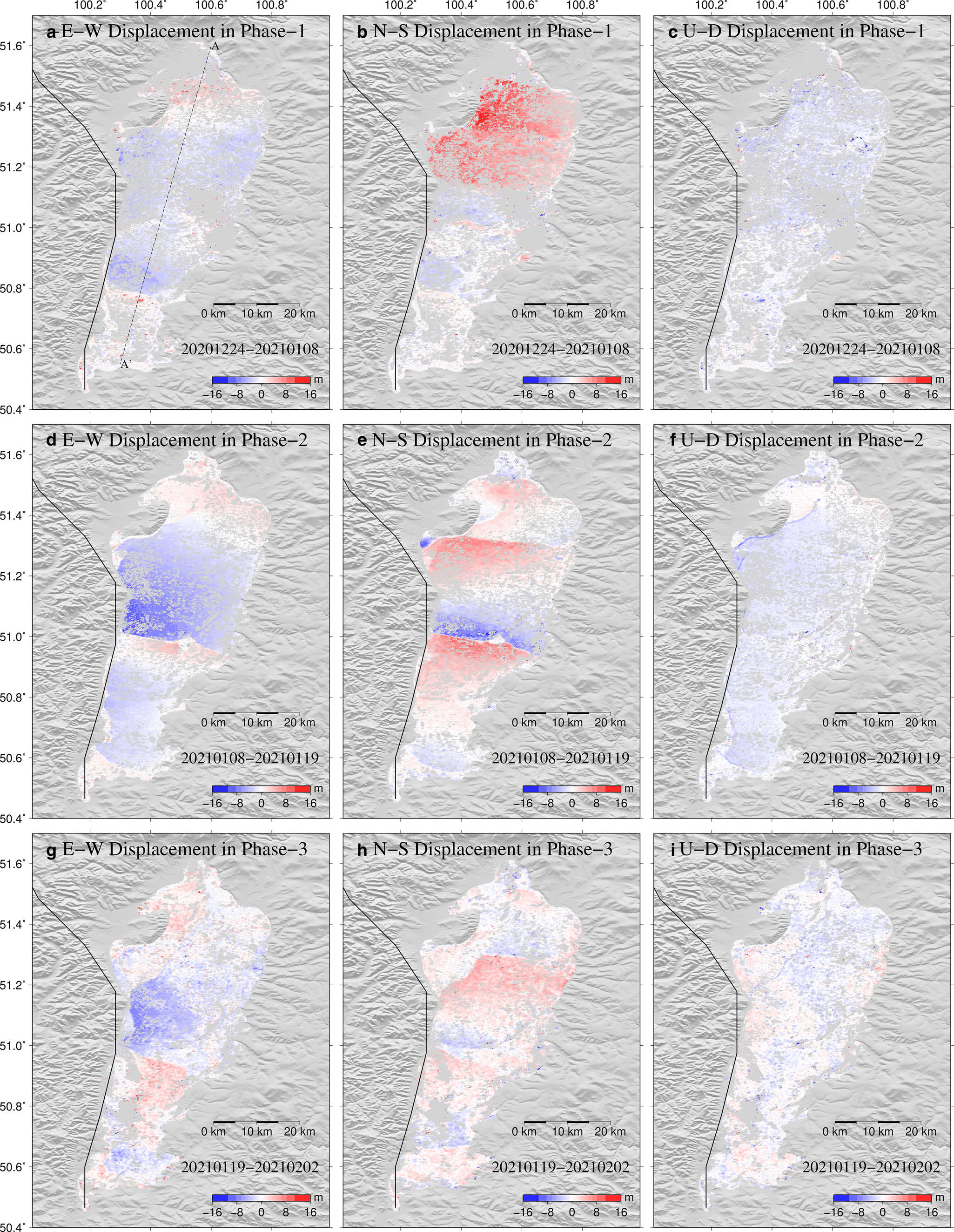
Fig. 8. The 3-D displacements estimated from Sentinel-1 and Sentinel-2 images for Phase-1, Phase-2 and Phase-3: (a–c) east–west, north–south, and relative vertical displacements in Phase-1; (d–f) east-west, north-south and relative vertical displacements in Phase-2; (g–i) east-west, north-south and relative vertical displacements in Phase-3, respectively. Black line indicates seismological fault associated with the 2021 Turt earthquake (Calais and others, Reference Calais2003).

Fig. 9. A comparison of the 3-D displacements on the three different components (E-W, N-S and vertical) along profile AA’ marked in Figure 8a. The black, blue and green points indicate Phase-1, Phase-2 and Phase-3, respectively.
4. Discussion
The pixel offset estimation from the Sentinel-1 SAR radar images and Sentinel-2 optical images provides measurements to derive 3-D displacement maps for large-scale lake ice motion. In previous studies (e.g. Berg and others, Reference Berg, Dammert and Eriksson2014; Andersen and others, Reference Andersen, Kusk, Boncori, Hvidberg and Grinsted2020), the DInSAR technique was used to explore changes in glaciers and sea ice, suggesting that the scattering features of the ice surface is coherent. However, there is low coherence between SAR scenes over lake ice in this study; thus interferometry could not be applied (for details of InSAR result, see Fig. S8), implying that the lake ice scattering properties of Khovsgol Lake may be different from the glacier and sea ice. A possible explanation for this is that the ice of the Khovsgol Lake surface is wet, resulting in large changes in surface scattering properties. Unlike the InSAR method, the POT method with intensity tracking performs well in all three phases in this study. Therefore, POT may be more appropriate in other fresh water lake ice applications. In addition, the Sentinel-2 optical imagery with four bands can be used for the POT analysis, and we find that Band 4 is the optimal band (relative to Bands 2, 3 and 8) for monitoring lake ice motion according to the tradeoff between spatial resolution and precision, which is different from the optimal band for ground deformation monitoring (He and others, Reference He, Feng, Feng and Gao2019a, Reference He, Wen, Xu and Chen2019b). We note that there are apparent relative differences in residuals from Phase-1 to Phase-3 in the optical POT measurements (Figs S4–S6). The residuals in Phase-3 seem much higher than Phase-2. We suspect this difference may arise from the ice motion direction (southward) or changes in ice surface scattering properties. The Sentinel-1 and Sentinel-2 imagery analyses both reveal common changes in the lake ice with different viewing geometries, but neither Sentinel-1 nor Sentinel-2 can individually reveal the complete characteristics of the lake ice motion in each phase. With these POT observations from both Sentinel-1 SAR and Sentinel-2 optical images, we are provided a rare chance to construct 3-D maps of the lake ice motion with a mean precision of <2.2 m as shown in Figure 8.
The 3-D displacement maps illuminate the complex spatiotemporal response of the ice motion of Khovsgol Lake. The limited availability of 3-D observations has heretofore greatly restricted research on ice motion. For instance, some investigations of sea ice or mountain glaciers only derived the ice flow velocity and direction and simply evaluated the inshore tide direction or glacier tongue motion along the gravity descent direction (e.g. Marbouti and others, Reference Marbouti, Eriksson, Dammann, Demchev and Antropov2020). To some extent, using only horizontal displacements hinders further insights into ridge dynamics and the relationships among ice thickness, convergence and ridge development, and resulting size, density and morphology of those ridges (Marbouti and others, Reference Marbouti, Eriksson, Dammann, Demchev and Antropov2020). In Phase-1, the maximum horizontal displacements in the E-W and N-S directions can reach 5.2 and 12.2 m, respectively; in Phase-2, the maximum horizontal displacements in the E-W and N-S directions can reach 10.3 and 8.7 m, respectively, and a maximum vertical displacement can reach 4.6 m; in Phase-3, the maximum horizontal displacements in the E-W and N-S directions can reach 6.6 and 5.8 m, respectively. In comparison to the 8–10 m displacements of the E-W and N-S components, most of the vertical displacements of 0–2 m are much smaller and under the precision of 2.2 m, suggesting that the movement of the lake ice in a vertical direction can be neglected. The 3-D lake ice motion shows a block pattern that fluctuates in the horizontal directions, particularly the N-S component.
In addition, the 3-D displacement profiles in Figure 9 show both large-scale fluctuations and small-scale periodic fluctuations of ice flow in each period, with the fluctuations occurring on spatial scales of several to tens of kilometers, as well as a relative displacement change of more than 4 m. The differences between these 3-D maps reveal that the lake ice experiences complex spatiotemporal dynamic changes. However, no such large-scale 3-D displacements associated with ice motion have been reported to date. That is, the 3-D displacement maps from remote-sensing images could be useful for quantitatively analyzing lake ice motion with reliable and high-density observations.
The movement of lake ice is a dynamic process governed by local climatic conditions (including temperature and wind), seiche waves, hydrological systems and precipitation. Lake ice motion is commonly accompanied by a series of physical phenomena, such as cracking, collisions, buckling, ice heaving and ice jacking (e.g. Kavanaugh and others, Reference Kavanaugh2019). Among these different features, pressure ridges are the predominant topographical surface structures and generally connect two points on land on either side of a lake or bay mouth. Therefore, the distribution and variability of ridges are important for quantifying ice displacement changes and their stress interactions (Duncan and others, Reference Duncan2018; Zhang and others, Reference Zhang, He, Hu and Liu2021). As shown in Figures 2–7, there are a series of large-scale displacement gradients in Phase-1 to Phase-3, and associated surface textural changes can be found in the Sentinel-2 optical intensity images (as shown in Figs S9–S11). In Figure S9, we show the ice surface features surrounding the R1–R5 from the two Sentinel-2 intensity images (i.e. dates on 24 December 2020 and 8 January 2021) and the locations of R1–R5. By comparing the two intensity images, we show that the locations of R1 and R5 change their surface texture, i.e. a new clear texture line appears in the secondary intensity image on 2 January 2021. However, other locations of large displacement gradients, such as R2, R3 and R4, do not show similar changes in the surface texture. In comparison to Zhang and others (Reference Zhang, He, Hu and Liu2021), our results indicate that the POT observations from Sentinel-1 SAR images is also sensitive to detect ice movement as well as Sentinel-2 optical images, and both of which can complement the mapping of ice motion features in intensity images using traditional remote-sensing classification techniques.
As shown in Figure 8, Khovsgol Lake is elongated in the N-S direction, the water flows from north to south, and the large pressure ridges cross the lake with an E-W strike. Several folded ridges are observed in the northern part of the lake during Phase-1 (Fig. 8b). During and after the Turt earthquake (i.e. Phase-2 and Phase-3), a large overlapping ridge across the island formed in the middle part of the lake (Figs 8d–i). Most of these large pressure ridges appear in the northern and middle parts of Khovsgol Lake. As shown in Figure 10, the northern and middle parts of Khovsgol Lake are characterized by relatively deep bathymetry (depths exceeding 250 m; Kouraev and others, Reference Kouraev2016), and the relative relief of the basement topography is 700 m (Krivonogov and Safonova, Reference Krivonogov and Safonova2017). The steep gradient changes between the bathymetry and basement topography correspond to the locations of large pressure ridges. One possible explanation for this is that after the formation of the ice cover, the heat flow from sediments decreases while the surface cooling rate increases (Kirillin and others, Reference Kirillin2012); thus, a high basement topography corresponds to fast cooling. Therefore, the general pattern of pressure ridges should depend on the lake bathymetry, the tectonic structure in the vicinity of the lake, and the morphology of the lakebed. In addition to the general pattern described above, the pressure ridges also migrate spatially, as demonstrated in Figure 9, which could be affected by Coriolis acceleration, seiche waves and internal waves (Kirillin and others, Reference Kirillin2012). However, developing a quantified forward model of the fundamental physical processes responsible for pressure ridges remains challenging due to insufficient observational information.

Fig. 10. The bathymetry (a), and basement topography of Khovsgol Lake (b). The red beach ball represents the focal mechanism solution and location of the 2021 Mw 6.7 Turt earthquake.
Large-scale lake ice motion associated with the 2021 Mw 6.7 Turt earthquake is revealed in the 3-D displacement maps. In this study, we processed the ice movement before, during and after the seismic event. The ice displacement magnitude is about two times larger during Phase-2 when the seismic event occurred compared to the magnitude of displacement before or after the event, particularly in the E-W direction. As shown in Figures 8d–f, large E-W lake ice displacements can be seen in Phase-2; such displacement patterns and large displacement magnitudes are not found in Phase-1 and Phase-3 (Figs 8a–c, g–i). Given that the temporal resolution of these three phases (Phase-1 to 3) is 10–15 d, we also compare the displacement in Phase-2 (during the period between 7 January 2021 and 19 January 2021) with the available ice movement results in the time window of 25 December 2018 to 19 January 2019 including the POT observations from the Sentinel-1 SAR and Sentinel-2 optical images and their relative 3-D displacement maps (as shown in Figs S12–13). Previous studies have suggested that the formation of lake ice in Tibet is strongly correlated with air temperature (Gou and others, Reference Gou2017; Li and others, Reference Li, Li, Wang and Hao2020). Assuming that boreal lakes have the same correlation feature of lake ice formation, this indicates that the lake ice motion in a similar time window but in different years should be approximately equal given similar temperature conditions. The mean local temperatures for Khovsgol Lake during the two periods, i.e. 25 December 2018 to 19 January 2019 and 7 January 2021 to 19 January 2021, are −26 and −21°C, respectively (https://www.ncei.noaa.gov/maps/daily/). Although the later period is 5°C warmer, both of these mean local temperatures are below-freezing, which is conducive to lake ice freezing. However, the 3-D displacements in Phase-2 (i.e. period between 7 January 2021 and 19 January 2021) show a 2–3 times magnitude compared to the period between 25 December 2018 and 19 January 2019. Therefore, these results suggest that the 2021 Turt earthquake may have had an impact on the ice motion of Khovsgol Lake. Different from the large N-S ice motion in the northern part of the lake in the Phase-1, the 2021 earthquake caused a large westward horizontal motion and obvious N-S displacements in the whole lake. The 2021 Mw 6.7 Turt earthquake occurred just beneath the northern part of Khovsgol Lake at a focal depth of 11.5 km (Fig. 10). The initial focal mechanism generated by the USGS suggests that the main nodal plane of the seismogenic fault is 219°/60°/–78° (strike/dip/rake angle), implying normal slip striking SSW with a high WNW-facing dip angle. Therefore, the surface displacement in response to this normal faulting event should be predominant in the E-W components, causing major water oscillations along the surface displacement directions in such an enclosed lake. As shown in Figures 8d–f, the lake ice displacement with an E-W direction is strongly related to the slip direction of this earthquake.
How the ice moves in response to the hydraulic and hydrodynamic processes associated with earthquakes is still poorly understood. Tsunami and seismic seiche are two possible mechanisms for explaining the hydraulic and hydrodynamic processes when considerable water oscillations are triggered by an earthquake occurred beneath a lake. Tsunami waves and seiche waves are often categorized together, but with two major differences. A tsunami is a large and destructive wave, and it is generally caused by a disturbance in the ocean, such as an earthquake or a volcanic eruption. Enormous tsunamis have been observed worldwide due to megathrust earthquakes, such as the 2011 Mw 9.0 Tohoku-Oki earthquake and the 2017 Mw 7.8 Palu earthquake (Mori and others, Reference Mori, Takahashi, Yasuda and Yanagisawa2011; Gusman and others, Reference Gusman2019). A seismic seiche is a short period standing wave formed when seismic waves pass through an enclosed or partially closed body of water in a lake; these characteristics distinguish seiche waves from tsunamis caused by coseismic deformation (McGarr, Reference McGarr and Gupta2011). To date, only a few seismic seiches have been recorded due to a lack of quantitative data, e.g. tide gauge records (Wang and others, Reference Wang, Holden, Power, Liu and Mountjoy2020). Existing reports have demonstrated that ice cover does not prevent seiche oscillations (Sturova, Reference Sturova2007; Zyryanov, Reference Zyryanov2011). However, a tsunami can also excite a seismic seiche in an enclosed basin such as a lake, and the tsunami is referred to as the initial wave produced by coseismic displacement from an earthquake, whereas the seiche is the harmonic resonance within the lake (Ichinose and others, Reference Ichinose, Anderson, Satake, Schweickert and Lahren2000). Limited to the temporal resolution of our imaging geodesy observations, both a tsunami and a lake seiche are possible explanations for the ice movement in the 2021 Turt earthquake. Seiche waves may continue for several days after a tsunami, and this long period of water oscillation can contribute to lake ice motion. In addition, there are also new N-S-striking pressure ridges formed, as shown in Figures 4 and 7. Therefore, we suggest that the seismic seiche was the driver of lake ice movement, and this study reports the possible formation of a rare seismic seiche recorded by lake ice.
5. Conclusion
We obtained the displacement field of the ice on Khovsgol Lake before, during and after the 2021 Mw 6.7 Turt earthquake by employing both Sentinel-1 SAR and Sentinel-2 optical remote-sensing data based on the intensity tracking method. We found that the classic InSAR technique was not suitable for monitoring lake ice motion due to loss of coherence, and we also found that Band 4 of the Sentinel-2 optical data was optimal for detecting ice displacements. Combining the available measurements with different viewing geometries, we derive 3-D displacement maps with a precision of <2.2 m in each period. Among these three periods, the 3-D lake ice displacement magnitudes in Phase-2 were much larger than those in the other two phases, particularly given the large E-W displacement of −10.3 to 5.2 m and the N-S displacement of −8.7 to 8.5 m, both of which possibly corresponded to the formation of a seismic seiche caused by a normal faulting event striking parallel to the long axis of the lake. In addition, our 3-D maps reveal that pressure ridges may have changed dynamically in response to this earthquake. The 3-D displacement maps of Khovsgol Lake ice presented in this study not only help us to further understand the properties and stability of lake ice for local transport safety but also provide new observations for the development of lake-ice models.
Acknowledgements
We thank the Scientific Editor Matthew Siegfried, the Associate Chief Editor Hester Jiskoot and three anonymous reviewers for their constructive comments. The Sentinel-1 SAR (https://scihub.esa.int/) and Sentinel-2 optical (https://earthexplorer.usgs.gov/) data were provided by the ESA through their open data policy. Most figures were plotted using Generic Mapping Tools (GMT). This work is supported by the National Natural Science Foundation of China (42174004, 41704005 and 41974004), and the National Key R&D Program of China (2019YFC1509204).


 Open access