Introduction

Investigations of the mass balance of the Hintereisferner began in the autumn of 1952, when Schimpp (Reference Schimpp1958, Reference Schimpp1960) placed 54 wooden stakes in eleven profiles across the glacier and surveyed them several times between February 1953 and September 1954. In the spring of 1954 an additional 40 stakes were placed by Reference RudolphRudolph (in press) and ablation and accumulation measured for one year, as well as the discharge from the glacier. Since the results from three precipitation gauges within the drainage area were available (Reference HoinkesHoinkes, 1954), it became possible to apply the mass balance equation

for the hydrological year 1 October 1953 to 30 September 1954. (N=total precipitation, A=discharge, V=total evaporation, R=net accumulation, B=net ablation.)

Beginning from the autumn of 1954 the network of stakes was kept under continuous observation on a somewhat reduced scale by Reference HoinkesHoinkes (1959). Comprehensive studies of the winter snow cover at the end of the hydrological winter half-year began in the spring of 1955, which were chiefly used to determine the total precipitation (Reference Hoinkes and LangHoinkes and Lang, in press [a]) for the drainage area. This could be done to the best advantage during the hydrological years 1957–58 and 1958–59, when a recording stream gauge was operating at the same spot where the discharge had been measured in 1954. In the summer of 1956 an additional precipitation gauge was set up; beginning from the autumn of 1959 a fifth gauge became available.

The drainage area of the stream gauge is shown in Figure 1. It comprises 26.62 km.², 58 per cent of which was ice-covered in 1959, i.e. Hintereisferner 9.97 km.², Kessel-wandferner 4.06 km.², slope glaciers 1.42 km².Footnote * The average height of the drainage area is 2,981 m., the stream gauge as the lowest point is situated at 2,287 m., the highest peak, Weisskugel, reaches 3,739 m. For the periods of the I.G.Y. 1957–58 and the I.G.C. 1959 the number of ablation and accumulation stakes was raised to a total of 117, 35 of which were placed on the Kesselwandferner. The determination of the mass balance of the glaciers within the drainage area for the hydrological years 1957–58 and 1958–59 was dealt with in detail in a report by Reference Hoinkes and LangHoinkes and Lang (in press [b]). Again two methods could be used, since the constituent parts of the mass balance equation were measured directly. Only the total evaporation remained to be estimated. The comparison of the best estimates available with the value calculated from V = N−A−(R−B) served as a check for the reliability of the measured quantities N, A and (R−B). It is, therefore, highly advantageous to measure precipitation and discharge at least for some years in addition to accumulation and ablation. Since the autumn of 1959 the observations have continued, again on a reduced scale, to the present date.

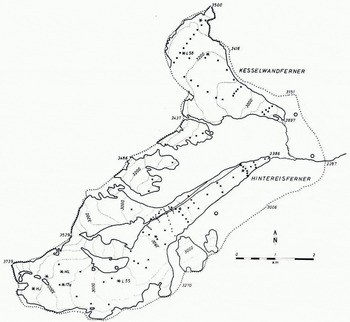
Fig. 1. The drainage area (26.6 km.²) of the Hintereisferner and the Kesselwandferner, Ötztal Alps. Heights in metres a.s.l., interval of contour lines 100 m. Positions of ablation stakes (●), snow pits (★) and rain gauges (◦) are shown for 1959

For the period 1957–59 the most complete data are available, and these are therefore the most suitable data from which to start to interpret the observations collected in previous and in following years. These observations were, as in most cases of mass balance studies, restricted to net accumulation and net ablation. The following remarks, therefore, will deal mainly with the interpretation of such observations, according to the experience gained on the Hintereisferner. A report about measurements of run-off from the glaciers is in preparation.

Net Ablation of Ice

Ablation stakes on the Hintereisferner were placed, as can be seen from Figure 1, in several cross profiles, connected through one longitudinal profile. Until 1957 square stakes (3×3 cm., length 1 m.) were used, most of which were then replaced by white round stakes of hard wood (diameter 2 cm., length 2 m.). The two types of stake could be joined together by means of metal bolts or sockets respectively. As long as the boreholes were deeper than about one metre, good ablation values could be obtained. This was checked by measuring the depths of adjacent bore holes not containing stakes over periods of several days. With a sufficient number of properly set ablation stakes it is possible to measure total net ablation of ice for a whole ablation season with an accuracy of better than ± 5 per cent. A number of about ten ablation stakes per square kilometre is considered as “sufficient”. This was proved by the results of 30 additional ablation stakes, placed on a surface of 1 km.², which have been used since 1957 by W. Ambach for studies of surface movement.

The values of net ablation of ice for each ablation season were entered on maps at a scale of 1:10,000, and lines of equal ablation were drawn at intervals of 50 cm. of ice. Figure 2 shows the analysis of net ablation for the 1954–55 ablation season, which, according to Table 1, had the smallest loss of ice in the period 1952 to 1961. Areas between single lines were measured by planimeter, multiplied by the respective average ablation value and added up, to give the total net ablation in cubic metres of ice. Detailed calculations and maps were published by Reference RudolphRudolph (in press) for the 1953–54 ablation season, and by Reference Hoinkes and LangHoinkes and Lang (in press [b]) for the 1958 and 1959 ablation seasons. The zero-line of ice ablation separates the area with unequivocal net mass loss from the area where there might be either gain or loss of mass. Above the zero-line of ice ablation begins the usually narrow zone of superimposed ice, after which the glacier remains covered with either old snow or firn until the end of the ablation season. The superimposed ice, by thorough inspection, can be distinguished from older glacial ice because of its peculiar structure (Reference HoinkesHoinkes, 1956). Detailed studies of the formation of superimposed ice were carried out on the Hintereisferner by Reference AmbachAmbach (1961). The zero-line of ice ablation can be, but is not necessarily, identical with the firn line or zero-line with respect to the mass budget. Nevertheless, the zero-line of ice ablation is considered as a fundamental line with clear conditions, i.e. net mass loss below it, which can unmistakably be identified by means of stake observations. It changes its position on the glacier from year to year, thus enlarging or reducing the area with comparably low albedo. In Figure 2 the lowest position of the zero-line of ice ablation is shown at the end of the budget year 1954–55, together with its highest position at the end of the budget year 1958–59 (dotted line). The corresponding areas with ice ablation were 2.58 km.² (1955) and 4.30 km.² (1959), as can be seen from Table 1. Within the nine years October 1952 to September 1961 the Hintereisferner lost a total of 64.55×10⁶m.³ of ice or 58.10×10⁶m.³ of water. The average annual ice loss amounts to 7.17×10⁶m.³ (6.45×10⁶m.³ of water) on an average area of 3.35 km.², viz. an average net ablation of 214 cm. of ice or 193 cm. of water per year.

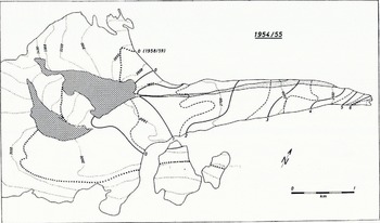
Fig. 2. Net ablation in metres of ice, Hintereisferner, budget year 1954–55. During the period 1952–61 the zero-line of ice ablation was in its lowest position in 1954−55, and in its highest in 1958–59 (indicated by heavy dotted line)

Table I. Mass Balance of the Hintereisferner, 1952/53 to 1960/61

Net Accumulation

Investigations of net accumulation in deep pits began on the Hintereisferner in the summer of 1955, and were extended to the Kesselwandferner in the summer of 1956. The water equivalent of the snow was measured with a snow sampler (area 50 cm.², length 50 cm.), which was weighed with a steelyard (5 g. corresponding to 1 mm. of water). In a short preliminary report about this work (Reference HoinkesHoinkes, 1957) it was stated that the typical distribution of density with depth, as found in the winter snow cover, showing a minimum at the bottom and a maximum somewhere in the middle of the layer, is preserved for many years. For this reason it can be used as a means for the detection of annual boundaries, together with changes in grain size and colour. The revised results of both deep pits are given in Figure 3 back to the budget year 1950–51, and a definite relation between both accumulation areas can be deduced. This valuable result was confirmed during the budget years 1957–58 and 1958–59, when five pits on the Hintereisferner and six pits on the Kesselwandferner were dug, some of them down to the 1956 horizon (Reference Hoinkes and LangHoinkes and Lang, in press [b]). Some additional values could be obtained from accumulation stakes, the readings of which were converted into water equivalent, using densities from nearby pits. Net accumulation values for a few selected points on the Hintereisferner and for the point L 58 on the Kesselwandferner, covering the whole period 1952–53 to 1960–61, are shown in Figure 4. There is a well pronounced increase in net accumulation between 3,100 m. and 3,300 m. a.s.l. and only a slight increase within the highest firn basins, which extend to 3,400 m. The relation net accumulation versus height was analyzed for each budget year; Figure 5 shows the limits for high (1954–55) and low (1957–58) net accumulation for the period under consideration.

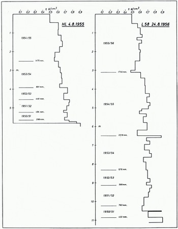
Fig. 3. Net annual accumulation for deep pit HL, at 3,170 m. on the Hintereisferner, and deep pit L 58, at 3,240 m, on the Kesselwandferner. Depth in metres, water equivalent in millimetres

Fig. 4. Net annual accumulation for selected sites on the Hintereisferner and for point L 58 on the Kesselwandferner for the period 1952–53 to 1960−61. Millimetres of wafer

In order to get the total net accumulation for a budget year, it was ctried at first to multiply the average net accumulation in steps of 100 metres by the corresponding glacierized area. By adding up for the two budget years shown in Figure 5, total net accumulations of about 7×10⁶m.³ of water (1954–55) and about 3×10⁶m.³ of water (1957–58) are obtained; the latter figure is obviously too high, because it does not fit the mass balance equation. The true, or at least better, values of net accumulation, according to Table 1, are only about 75 and 50 per cent, respectively, of the first estimates. This simple and frequently used method can be expected to give satisfactory results only if the measured net accumulation is truly representative of its height zone. This demand is not easy to realize, at least not on crevassed alpine glaciers, where pits are normally dug in basins rather than on ridges for safety reasons.

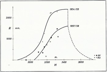
Fig. 5. The relation net accumulation (millimetres of water) venas height (metres) on the Hintereisferner and Kesselwandferner for a budget year with high (1954–55) and low (1957–58) net accumulation

As can be seen from Figures 6 and 7, no closed cover of old snow remained in the area of nourishment of the Hintereisferner and the Kesselwandferner in the autumns of 1958 and 1959. Areas having net accumulation of old snow from the current budget year are clearly distinguishable from areas where several layers of older firn snow are exposed to ablation. The border-line between old snow and firn snow should be called the old snow line; it is another fundamental line within which clear conditions, i.e. net mass gain, prevail. The “old snow line”or a line very close to it within which the water equivalent of the superimposed ice exceeds the ablation of firn snow, separates the area with positive economy from the area with negative economy. This is the exact meaning of the terms “firn line” or “firn limit”. The term “firn line” nevertheless seems to be somewhat unfortunate, because under conditions of retreating “firn line” (as in Figures 6 and 7) the “firn line” runs across the firn snow. It is open to question whether or not all observers distinguish between “old snow” from the current budget year and “firn snow” from budget years before, and therefore some might be tempted to identify as the firn line the beginning of the firn cover (i.e. the zero-line of ice ablation). The adoption of the term “old snow line”, which would be helpful in avoiding errors, as it would presuppose only the recollection of the meaning of the German word Firn (= of last year). Consequently Reference FlintFlint (1957) writes: “The process of growth and change is one of recrystallization, and the result is compact granular snow. Such snow, when more than one year old, is known as firn or névé”. The otherwise excellent definitions of the terms “old snow” and “firn”, given by Reference Armstrong and RobertsArmstrong and Roberts (1958), should require a short addition with respect to time. A lower density limit for firn “greater than 0.55” (Reference SharpSharp, 1960) does not seem very fortunate, because on polar glaciers the density of firn is frequently below 0.55 g./cm.³.

Courtesy Prof R. Finsterwalder

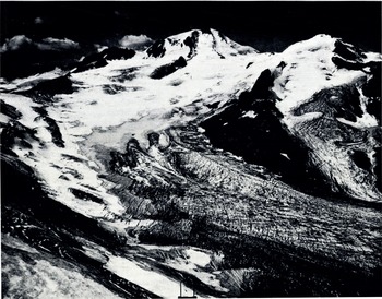
Fig. 6. The upper part of the Hintereisferner with the peaks Weisskugel (3,739 m.) and Langtau fererspitze (3,529 m., to the right). The transition zone: glacier ice—superimposed ice—firn snow from five years—old snow from the current budget year shows clearly. Photograph taken 6 September 1958, by Institut fib Photogrammetrie, Topographie and Allgemeine Kartographie, Technische Hochschule Munchen.

Photograph taken 30 September 1959 by H. Hoinkes

Fig. 7. The upper part of the Kesselwandferner with the peaks Fluchtkogel (3,500 m., left) and Kesselwandspitze (3,416 m., right). Typical accumulation patterns. Firn snow from five years exposed to ablation. White snow is old snow from the ending budget year.

Comparison of photographs taken in late summer of different years, reveals that the accumulation patterns are not distributed at random in single years, but remain rather stationary, changing more in size than in shape. This fact was clearly pointed out by Reference FriedelFriedel (1952); it is caused by differences in accumulation due to the action of the wind, and by different conditions for ablation due to slope, exposure, and possible duration of sunshine. Even avalanches might be responsible for certain patterns. The very existence of enduring accumulation patterns offered a means of improving the estimate of the true total net accumulation. All available photographs, sketches, and notes from different years were used for mapping the accumulation patterns. We had to make do with photographs taken from the surrounding mountains, but without doubt regular aerial photographs, taken as late as possible in the ablation season, would be the best basis for estimates of the total net accumulation, if combined with pit studies.

Figure 8, as an example, shows the mapping of net accumulation patterns on the Hintereis-ferner at the end of the budget year 1957–58. Seven grades were used, the different signatures indicating areas with the respective average net accumulation of old snow. Areas without a signature above the zero-Iine of ice ablation denote areas with firn ablation. Isolated patches without accumulation above the old snow line are found on crevassed ridges or bumps of the terrain (cf. Figure 6);Footnote * they are actually much more complicated than shown on the map. The size of these patches was drawn in such a way that ablation of firn and accumulation of old snow compensate each other. All the individual areas were measured with a planimeter, multiplied by their respective average water equivalents of the accumulated old snow, and added up in order to give the total net accumulation for the budget year in question. In the budget year 1957–58 the area with net accumulation of old snow was only 3.49 km.², the total amount 1.49×10⁶m.³ of water. Within the nine years October 1952 to September 1961 the average area with net accumulation of old snow was 5.99 km.², the average total amount accumulated 3.11 × 10⁶m.³ of water per year (see Table 1).

Fig. 8. Net accumulation of old snow on the Hintereisferner at the end of budget year 1957–58. Shadings indicate seven grades of net accumulation in millimetres of water

As an important consequence of enduring accumulation patterns which repeat themselves, a connection was to be expected between the net accumulation of a single representative spot within the area of nourishment, and the total net accumulation of the glacier for a certain budget year. This non-linear relation is shown in Figure 9 for the deep pit HL (3,170 m.) on the Hintereisferner. A similar relation holds between the annual net accumulation as found in the deep pit L 58 (3,240 m.) on the Kesselwandferner and the corresponding total net accumulation of the Hintereisferner. This result, which is now confirmed by the observations of nine years, enables a quick control of the total net accumulation of the Hintereisferner to he made. A corresponding relation exists between the net ablation on the tongue of the Hintereisferner in the height zone 2,700 to 2,800 m., and the total net ablation of the Hintereisferner (Fig. 1).

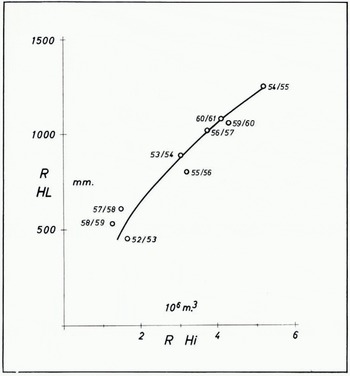
Fig. 9. Relation between net accumulation (millimetres of water) at point HL (3,170 m.) on the Hintereisferner, and total net accumulation on the Hintereisferner (millions of cubic metres of water). Budget years 1952–53 to 1960–61

Net Ablation of Firn

The difference between the total area of the Hintereisferner, and the sum of the areas with net accumulation of old snow and net ablation of ice gives the area with net ablation of firn. This area is usually quite small, except in years with a pronouncedly retreating old snow line, as for example 1957–58 (see Table 1 and Figures 6 and 7), when firn layers from several years become exposed to ablation over a comparatively large area. In such years the zero-line of ice ablation is retreating as well, causing firn ablation also below the final position of the zero-line of ice ablation, i.e. in the area between the zero-line of ice ablation of the preceding and the current budget year. This area is included in the area with ice ablation ; it might sometimes, as for example in the budget year 1957–58, reach considerable size. The density of the exposed firn layers was found to vary most frequently between 0.60 and 0.66 g./cm.³ ; the mean value 0.63 g./cm.³ was used for calculations of firn ablation. In years with an advancing old snow line, virtually no firn ablation occurs, as for example in 1953 to 1955 and in 1959–60. During the period 1952 to 1961 the average area of firn ablation between the zero-line of ice ablation and the old snow line was 0.72 km.², the average total amount of firn lost there had a water equivalent of −0 17x10⁶m.³ per year. The average total amount of firn lost below the zero-line of ice ablation is equal to −0.09 × 10⁶m.³ of water per year.

The Mass Balance

By subtracting the mass loss due to net ablation of ice and firn from the mass gain due to net accumulation of old snow one gets the mass balance of the whole glacier, which is shown graphically in millimetres of water for the whole surface of the glacier in Figure 10. In Table 1, for the sake of clarity, the mass balance is calculated separately for the area of the glacier covered with old snow or firn (above the zero-line of ice ablation), and for the area showing bare ice at the end of the budget year (below the zero-line of ice ablation) . Apart from practical reasons, this sub-division is justified by the appreciable differences in albedo as well as in the roughness parameter between the two kinds of surface. ‘I’he mass balance for the whole glacier is given in convenient form with respect to the old snow line. There is a large variation in the mass balance of more than ten millions of cubic metres of water between the most favourable budget year 1954–55 with a slightly positive mass balance, and the most unfavourable year 1957–58, which will be interpreted in terms of climatic conditions in another report (Reference Hoinkes and RudolphHoinkes and Rudolph, 1962).

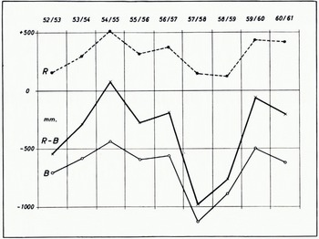
Fig. 10. Total net accumulation (R), total net ablation (B), and mass balance (R–B) in millimetres of water for the whole surface of the Hintereisferner, budget years 1952–53 to 1960–61

On an average, more than twice as much mass was used up by net ablation of ice and firn (6.71 × 10⁶m.³ of water or 667 mm. over 10.06 km.²) than was deposited on the glacier by net accumulation of old snow (3.11×10⁶m.³ of water or 309 mm. over 10.06 km.²). The average annual mass loss of the Hintereisferner in the period 1952–61 amounts to 3.60 × 10⁶m.³ of water, or 358 mm. of water over an average surface of 10.06 km.². The average area of nourishment (5.99 km.²) exceeded the average area of wastage (4.07 km.²) by 47 per cent. The average for the nine years is strongly influenced by the two unfavourable years 1957–59, when net ablation used up more than seven times as much mass (10.05×10⁶m.³ of water) than was deposited by net accumulation (10.38 × 10⁶m.³ of water) on an area of nourishment (3.45 km.²) which was only about half that of wastage (6.54 km.²). More than half (54 per cent) of the 32.45 × 10⁶m.³ of water lost in the nine years of observation were lost in the two most unfavourable budget years 1957–58 and 1958–59. By adding the budget year 1952–53 one gets a mass loss of almost three-quarters (71 per cent) of the total, viz. 7.66×10⁶m.³ of water, or 760 mm. of water over an average surface of 10.08 km.² per year. For the six remaining budget years 1953–57 and 1959–61 average net ablation of ice and firn (5.51 × 10⁶m.³ of water) was just 40 per cent in excess of average net accumulation of old snow (3.93×10⁶m.³ of water). The average annual mass loss was only 1.58×10⁶m.³ of water, or 157 mm. of water over an average surface of 10.05 km.². The average area of nourishment (6.92 km.²) was more than twice as large as the average area of wastage (3.13 km.²). In the best budget year so far, 1954–55, with slightly positive mass balance, the area of nourishment was nearly three times as large as the area of wastage (see Table 1 and Fig. 2).

A lowering of the mean position of the old snow line by about 120 m., down to a height of about 2,830 m., as in the budget year 1954–55, would be sufficient to bring the Hintereisferner back to equilibrium with respect to the mass balance. The old snow line was in its highest average position in the unfavourable budget years 1957–58 and 1958–59, when it receded to 3,120 m. During the six budget years 1953–57 and 1959–61 the average position of the old snow line was 2,885 m.; for the whole period 1952–61 it was situated at an average height of 2,950 m.

Estimation of Errors

A few remarks seem necessary with regard to the accuracy with which the mass balance components could be determined. Errors in field work on glaciers are hardly to be avoided, because bad weather conditions now and then prevent the collection of complete observations. Such gaps in the material have to be closed rather subjectively by interpolation or reduction. The calculation of total values from erroneous or not representative values may cause errors, the amount of which is not easy to estimate. For a few years we calculated the components of the mass balance with the largest and smallest possible values in order to get an idea of the possible deviations. This was done to the best advantage in the years with measured or recorded run-off from the glacier, i.e. 1953–54 (Rudolph, 1961) and 1957–59 (Reference Hoinkes and LangHoinkes and Lang, in press [b]). From these years we reached the conclusion that we were able to determine total net accumulation of old snow to about ± 10 per cent, total net ablation of firn to about ±15 per cent, and total net ablation of ice to about ±3 per cent. In the worst possible case, when the errors of the single components add up with the same sign, the final average error of the mass balance could amount to about ±0. 54× 10⁶m.³ of water (see Table 1). The actual error most probably will be smaller, because some compensation is to be expected.

Acknowledgements

Field work since 1955 and evaluation was sponsored mainly by the Österreichische Akademie der Wissenschaften and by the Hydrographisches Zentralbüro, both in Vienna. Final evaluations for the present report were supported by a grant from the Deutsche Forschungsgemeinschaft to one of us (R.R.). Special thanks are due to the numerous collaborators, mostly undergraduates and graduates from the University of Innsbruck, who offered their help on a voluntary basis. Of these chiefly H. Lang should be named, who contributed most to the field work as well as to the final discussions and conclusions.