


Introduction
Due to the magnitude of errors in the field measurement of the length of a line, one of the constraints in determining the strain-rates on glaciers is the length of time that must elapse before a remeasurement of distance is made. For strain lines ≤ 100 m, where the strain-rates are ≈ 10−11 s−1, the period between measurements is commonly a year.
One expression for strain-rate ε may be written:
where Δl = l 2 — l 1 — ½(l i + l 2), in which l1 and l2 are the original and final lengths, and Δt is the time interval between measurements.
It is now possible to avoid the repetitious direct measurement of line length by monitoring the quantity Δl continuously. In addition, the velocity Δl/Δt may be similarly monitored provided it is between certain specified limits. The line length need then be measured only once by a relatively simple method.
An experiment designed to test this procedure, using the Hewlett-Packard laser interferometer was carried out on Fletcher’s ice island T-3 during April and May 1973. At that time the island was gripped in the pack ice at lat. 83.7° N., long. 85.5° W.
Instrumentation
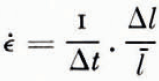
The following Hewlett Packard equipment was used (Fig. 1): one 5505A laser display unit, one 5500C laser head with tripod, one 10565B remote interferometer, two 10550B reflectors and mounts.
Additional materials and instruments included: two aluminum tubes 10 cm diameter, 4 m long, with an 8.3 cm diameter, 2 m long sliding inner tube fitted with an expansion clamping device and a top mounting plate (approximate total weight of each tube assembly, 21.8 kg), one 4 m long thermistor string, a barometer, hygrometer and thermometer mounted in a standard screen.
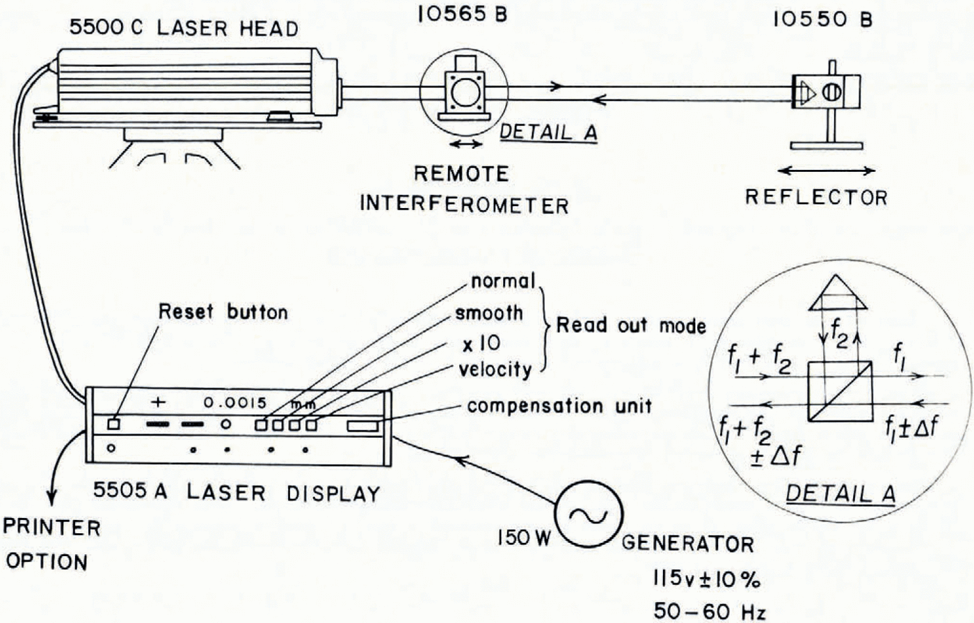
Fig. 1. Basic layout for the Hewlett Packard system 5526A linear interferometer.
To appreciate fully several aspects of the field operation of the instrument, it is necessary to review some principles of operation of the laser interferometer. The principles of the system, of which the present configuration (the linear interferometer) is the simplest, are outlined in Hewlett Packard Manual No. 05526-90001.
The laser is a low-power helium-neon unit which can therefore be powered by a small portable generator. A two-frequency principle allows the return beam to be depleted by up to 95% before an error signal is triggered. This feature permits considerable misalignment (or flutter) of the beam and thus facilitates setting the system up in the field. For this experiment an external (remote) interferometer and single reflector was used. On entering the remote interferometer (Fig. 1; delail A) the beam is split at the surface of a polarizing beam splitter, with one reference frequency (f 2) reflected from the corner cube mounted on the housing of the interferometer. The other frequency (f 1) is transmitted to the reflector and returns with a frequency shift, Δf, to be passed with f 2back along a common axis to the photo-detector block in the laser head.
Relative motions between the interferometer cube and the reflector cause a difference in the Doppler shifts in the frequencies of the returning beam. The difference between the frequency registered by the measurement photodetector and the frequency registered by the reference photodetector is monitored by a subtractor and accumulated in a fringe-count register. A digital calculator samples the accumulated value every 5 ms and performs a two-stage multiplication: one for refractive index correction and the other for conversion to inches or millimetres. The display shows on selection either distance or velocity. The distance shown on the laser display at any time is equal to the product of the laser (air) wavelength and the number of wavelengths of motion counted since the reset button was last depressed. The reset button also serves as the error-signal indicator. The ratio of the wavelength in air to that in vacuum is used in the calculation, and for normal conditions of use its value is o.ggg XXXX where the last four digits may be determined from the temperature, pressure,and humidity of the air. Neither the automatic compensator (model 5510A), nor the compensation tables, covered the appropriate range of conditions in the field, therefore it was decided to leave an arbitrary value of the last four digits set in the instrument (by thumbwheel switch control) and to correct later for the change in pressure, temperature and humidity. It turned out that this correction was negligible when rounding off readings in millimetres to the fourth decimal place. The stated accuracy is ±0.5 p.p.m. ±2 counts in the last digit; resolution in smooth or normal modes is 0.000 1 mm, in X 10 mode: 0.000 01 mm. The maximum allowable measuring velocity is 0.3 m s−1 above which the reset signal is triggered. This signal is also triggered when more than 95% of the signal is lost or when there is a tuning error. Rather than use a digital recorder, it was decided to record the readings manually from the display because of the periodically high rate of reset and the general lack of requirement for closely spaced data. Furthermore, the necessity of periodic realignment of the beam and of reading the pressure and temperature and ensuring a steady flow of air through the laser box, required an operator to be present continuously. Consequently, a shift system was used.
Operation of the System
The field arrangement is shown in Figure 2. To ensure stability of the laser, the tripod was mounted on the ice, through holes in the floor of the operating hut. The feet of the tripod were frozen into shallow holes in the ice. The laser head and tripod were surrounded by a thermally lagged box, access to the interior of which was gained by a side door. The remote interferometer and the two reflectors were mounted on adjustable posts consisting of the aluminum tube with the inner tube on top of which was attached a mounting plate. The posts were placed on wooden discs 6 in (15 cm) in diameter in holes 3.5 m deep, 8 in (20 cm) in diameter drilled in the ice. A slurry was then slowly poured around the outside of the tubes while the axis was held vertical. This was controlled by using the optical plummet of a theodolite aimed on a centre mark on the base cap of the tube and on a cross-hair mounted on the upper end of the tube. The tube axes were all finally set within 50” of are of the vertical. The two reflector posts were positioned at distances of 52.85 m and 99.76 m from the remote interferometer. Thermistors were frozen in beside the posts and measurements were taken until temperatures were restored to stable values: this took about 7 d. Before actual measurements with the interferometer were made the time lapse was about 10 d. Typical ice temperatures are shown in Figure 3.
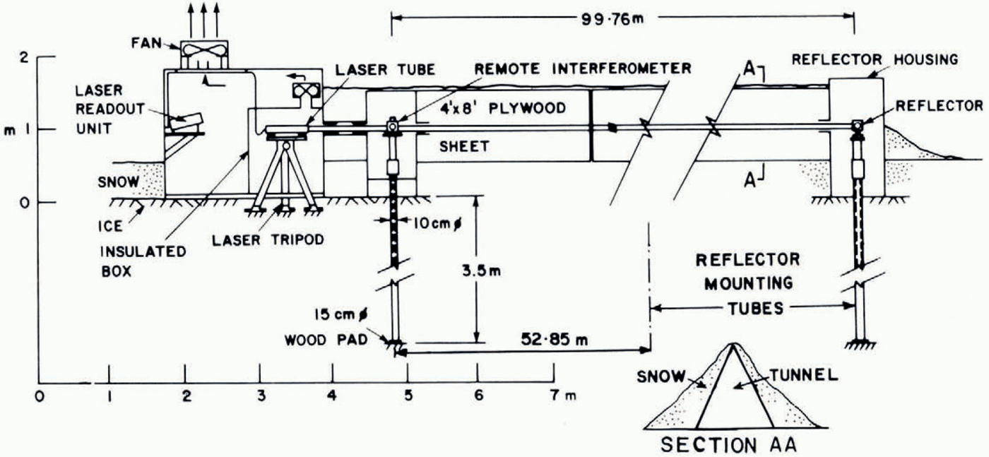
Fig. 2. Cross-section through field set-up of laser interferometer.
The inner tubes of the mounting posts could be clamped at any desired level by a rod and expanding cone system at the lower end and locked by a knurled ring at the upper end. For alignment, the laser head was pointed at the reflector, which was adjusted laterally and rotationally for maximum return signal. This was a long trial-and-error process as the horizontal circular adjustment on the tripod was not precise enough. The remote interferometer was then easily positioned and mounted in the beam path. The laser hut, remote interferometer, and reflector housing were linked by a tunnel made from 44 pairs of connected 4 ft X 8 ft (1.2 m X 2.4 m) plywood sheets set in the shape of an A-frame and covered by snow to reduce radiational heating inside the tunnel and stabilize temperatures along the path of the laser beam. The tunnel had the effect of sustaining a draft through the laser box even under very low wind. Under zero draft severe flutter of the laser beam—causing the error signal to be actuated—was attributed to heating of the air causing convection in front of the laser head. A system of fans was employed to induce draft when there was insufficient wind to produce a draft in the tunnel. In addition the tunnel allowed the experiment to be run under adverse weather conditions. Minor adjustments to the direction of the laser beam were made by rotating the rear levelling screw of the laser head, or by slight repositioning of the interferometer or reflector. The tolerance of the system to 95% beam loss contributed much to the final success of the experiment, because beam flutter was the single outstanding problem. As a result of this the longest period of continuous operation without a reset was about 4 h After switching on a period would usually be allowed to elapse until the system stabilized. Unacceptable flutter in the signal was corrected by draft regulation.
Fig. 3. Ice temperatures to 3 m depth.
For the longer measurement runs, display readings would be taken every minute, temperature and pressure every ten minutes. Humidity was automatically recorded in a meteorological screen and was mostly between 90 and 100%. Several shorter runs were made. A special experiment was run over a period of an hour where readings were recorded on tape every second simultaneously with gravimeter measurements taken near the north edge of the island.
Generally, with the successful runs the beam-alignment meter (indicating strength of signal) would indicate 7±0.5, whereas the cut-off signal strength for reset is 4.0. Since resets could occur even with this relatively high signal strength, it was deduced that larger fluctuations occurred in the signal of higher frequency than the meter could respond to. Alternatively, to explain this observation the relative velocity between the two points would have to exceed the specified maximum value (0.3 m s−1) but there is no evidence to support this.
Results
A 24 h run was made using the 99.76 m line, from 20.00 h 18 May to 20.00 h 19 May. Figure 4 shows the values of pressure, temperature, and humidity (measured in a Stevenson meteorological screen) as well as the instrument thumb-wheel setting XXXX at ten-minute intervals. Figure 5 shows the corrected time-displacement plot where each point represents the mean of ten readings taken at one minute intervals. The reset points were joined using separate plots of differences between readings versus time and interpolating to the reset time to obtain a difference value. Fluctuations much smaller than I h period are filtered out by the averaging process. Over the 24 h period the average strain-rate is (— 2.64±0.1) x 10−11 S−1. Figure 6 shows two other runs of shorter duration (4 h) along the same direction but for a distance of 52.85 m. As before the averaging has been done over intervals often minutes and it may be seen that an oscillation of period about one hour is present. Averaged over four hours both runs show a strain rate of (— 3.6±0.6) X 10−11 s−1.
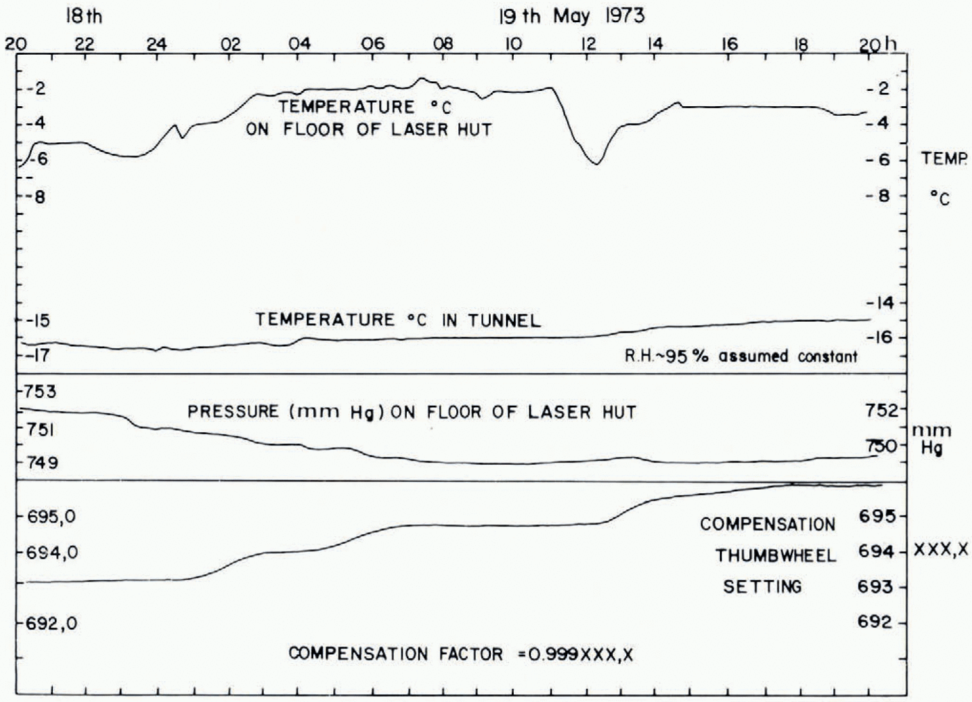
Fig. 4. Plot of temperature, pressure, nud compensation setting variations over a 24 h period, 18-19 May 1973.
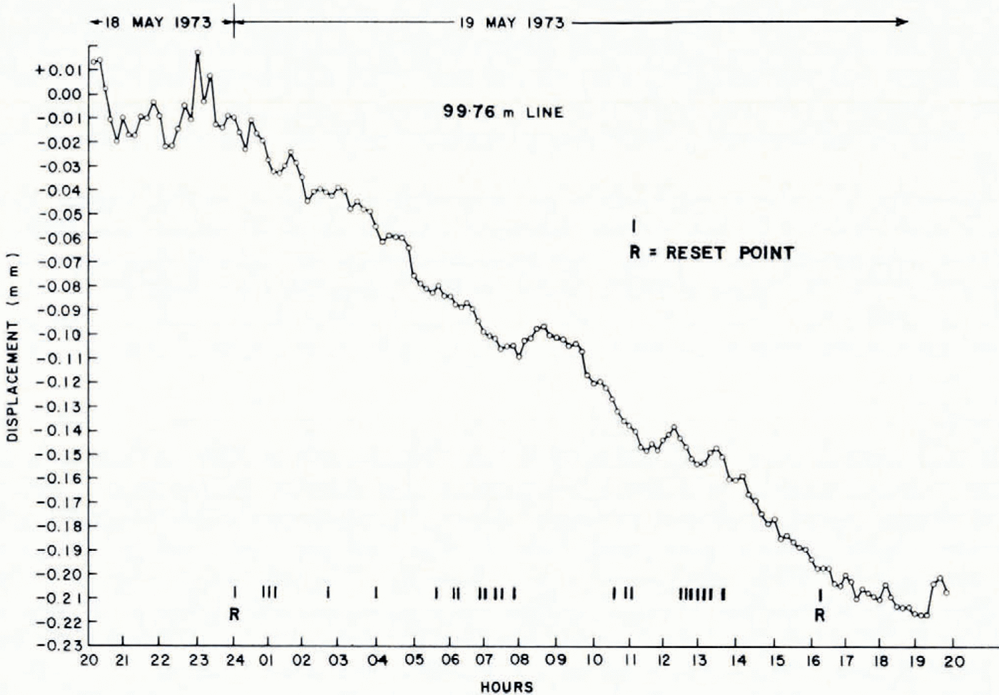
Fig. 5. Time-displacement plot for the 99.76 m line, 18-19 May 1973.
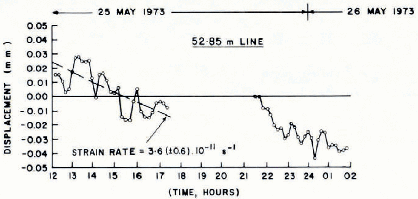
Fig. 6. Time- displacement plot for the 12. 85 m line, 25-26 May 1973.
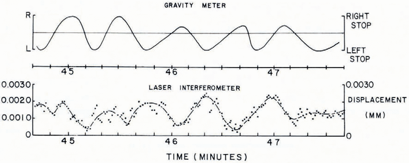
Fig. 7. Section of 1 h record showing laser interferometer readings and LaCoste and Romberg gravimeter readings. Individual laser interferometer readings (1 s intervals) are deviations (mm) from a curve joining 10 s running means.
Figure 7 shows a portion of the one-hour record during which the laser readings oscillated with an average period of 35 ±1 s. During the same interval the gravimetcr beam oscillated with an average period of 37 ±2 s, although the oscillations were not in phase.
Discussion of results
Figures 5 and 6 show, on the average, compressive strain-rates, if the oscillations due to flexing ol the island are filtered out. These average strain-rates are composed of a strain-rate of mechanical origin, one of thermal origin, plus “apparent strain-rates” generated within the experimental set-up. The following discussion is intended to show that tilting or sinking of the mounting tubes is not responsible in this case for generating an “apparent strain-rate”. of order 10−11 s−1.
-
(1) All tubes were completely frozen in to solid ice along the 3.5 ± 0.1 m buried length. so that the final orientations of their axes were within 50 arc seconds of being vertical. The vertical pressure transmitted through the wooden disc was less than the hydrostatic pressure in the ice by 0.02 MN m−2, therefore no downward creep could be expected. All tubes were identical in manufacture and placement; if vertical displacements could occur they would be identical.
-
(2) Tilting is considered most unlikely because:
-
a. the tubes were completely protected from radiational heating,
-
b. the average temperature of the upper 3 m of ice was about —22° C.
-
c. all the five runs which exceeded four hours for either line length clearly gave compressive strain-rates of the same order of magnitude: variations may easily be caused by pressure changes in the pack ice,
-
d. an independent adjacent strain net (Reference Holdsworth, Traetteberg and Karlsson.Holdsworth and Traetteberg, [1974]) measured with a geodetic tape, showed strain-rates (average over 10-20 d) of 10−11 s−1 (irregularities appear due to the system of surface cracks in the ice),
-
e. assuming a tube tilt of 50 arc seconds with 3.5 m of tube buried in the ice, the average normal stress (above hydrostatic) exerted by the tube on the ice is inadequate by several orders of magnitude to cause tube displacements sufficient to produce an “apparent strain-rate” of 10−11 s−1,
-
f. we assume that the measured strain-rates are produced by a mechanical stress and a thermal stress, then the mechanical stress would be at least 0.01 MN m−2, using the idealized creep curves of Reference BuddBudd (1969) . Taking the average thickness of the island and the sea ice as 30 m and 3 m respectively, (Reference Holdsworth, Traetteberg and Karlsson.Holdsworth and Traetteberg, [1974]) this implies that pack-ice pressures could be at least 0.1MN m −2 (1 bar). Such a value is quite reasonable Parmerter and Coon, in press).
Conclusions
Application of this system could be extended to sea or lake ice provided the mounting posts are redesigned. For land-based glaciers, where there is a large firn depth, the tubes must be sunk deep enough to prevent tilting of the tubes. The instrumentation could be set up in a deep, covered trench. Because in this case strain oscillations are not expected, a much smoother displacement-time plot should result, enabling strain-rates to be obtained over shorter periods of time than reported here.
The aser unit operates successfully at air temperatures below 0° C Pre-heating may be achieved using an infra-red lamp; once the unit is switched on self heating will take place. Heat must be conducted away from in front of the laser head, or severe flutter of the beam will result. Frosting of the optical surfaces is a problem if the remote interferometer and reflector are left in position for more than one day.
Under enclosed conditions or in stable air without precipitation, the maximum practical distance between the interferometer and the reflector is about 100 m, with the laser output gain at the highest level. The beam may be rotated through a right angle by changing the position of the reflector assembly on the remote interferometer and remounting the cube rotated through 90°. In this way, two orthogonal strain-rates may be measured at closely spaced intervals of time. Another mounting post is needed for this, but the same reflector may be used.
Acknowledgements
I thank T. J. Hughes, J. Kruus, A. Traetteberg, and R. Weaver for consultation and help with the experiment. Logistic support was provided by the Polar Continental Shelf Project, Department of Energy Mines and Resources, Ottawa, Ontario, and the Office of Naval Research, Barrow, Alaska.


