

Cambridge Austerdalsbre Expedition, Paper No. 6
1. Introduction
In 1956 the Cambridge Austerdalsbre Expedition was studying the formation of wave ogives at the foot of the Odinsbre ice fall in Norway. 1 , Reference Nye 2 , Reference Nye 3 For this purpose a line of 23 stakes running longitudinally down the glacier was set up (Fig. 1), and the changes in the distances between the stakes were measured over a period of one month. It was then possible to deduce the longitudinal strain-rate in the ice as a function of the distance down the glacier; this was the main purpose of the experiment and the results are fully described in reference 3. The present paper is concerned with some additional measurements made on the stake system. Besides finding out the longitudinal component of strain-rate we wanted to have some information about the other components of the strain-rate tensor at a few representative points down the stake line. We therefore set up the five squares of stakes shown in Fig. 1 centerd on Stakes 3, B, C, D and E. By measuring the sides and diagonals of these square patterns at intervals over a period of one month it was possible to calculate with considerable accuracy all components of the rate of strain tensor at the five center points. The number of quantities measured at each square is greater than the number of unknowns to be derived from them, and the method used to calculate the strain-rate components from the data may be of some interest.

Fig. 1 Map of the stake system at the foot of the Odinsbre ice fall showing the measured intervals, the directions and magnitudes of the principal stresses, the horizontal component of velocity, the directions of maximum surface slope and the positions of the crevasses
Having obtained the strain-rate components we proceed to calculate the principal strain-rates and, by using the measured flow law of ice, the principal stresses. It so happened that the main stake line skirted the edge of an extensive crevassed area on its western side. It is therefore possible to compare the direction of the crevasses with the direction of the principal strain-rates, and to see whether the crevasses are associated with tensile stresses. Although the experiment can be used for this test of the theory of crevasse formation, it was not specifically designed for the purpose; if it had been, a different location would have been chosen.
2. Measurements
The relation of the stake line to the ice fall is shown in the map which appears in Fig. 1 of reference 3; Figs. 13, 14 and 15 of the same paper show photographs of the stake system. The method of making the measurements on the squares has already been described in reference 3 and the details need not be repeated here. In brief, all the intervals shown by dotted lines in Fig. 1 of the present paper were measured three or four times in August 1956; certain corrections were applied, and the average rate of stretching

where l 1 and l 2 are the initial and final lengths of a stake interval and Δt is the time interval.
3. Reduction of Results
Fig. 2a shows a square pattern of five stakes. Ideally, the outline is a perfect square with one stake in the center. The x axis is along one diagonal and points down the glacier; the z axis is along the other diagonal, and the y axis is normal to the glacier surface. The measurements give 8 values of
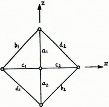
Fig. 2a Ideal stake pattern

Fig. 2b
If the object had been simply to measure strain-rates, we could have dispensed with the stake at the center;
In fact it was not always possible to make the arrays as near to perfect squares as we should have liked, because the geometrically correct position of one or more of the stakes turned out to be in a crevasse. The resulting compromise meant that the angles were not quite 45° and 90°. The worst case was the square centerd on C, where the angles of the various pairs of intervals at the mean survey date, measured clockwise from the direction C-CE, were

When averaged, these give
If the axis of reference is now rotated anticlockwise by 0.5° we obtain
and the greatest misalignment in angle from the ideal values 0, 45, 90, 135° is 3°. We accordingly place Oz at 0.5° anticlockwise from the line C-CE; Ox is placed at right angles to Oz.
This case has been chosen for illustration because it is the worst. The corresponding angles for the other four squares are given in the Appendix set out in the same way. Corresponding to the misalignment of 3° noted above for Square C, the misalignments for the other four squares 3, B, D and E were 1.5, 1, 2 and 0° respectively.
The procedure is, accordingly, first to choose the x and z axes for each square in such a way as to make the directions a, b, c, d, as close as possible to 0, 45, 90 and 135°. We then assume that the measured values correspond exactly to these ideal directions. The 8 measured strain-rates

Table I The Average Rate of Stretching of the Measured Intervals in August 1956 (yr.−1)

Corresponding values are then averaged in the next line of the table to give
The principle of least squares is now used to deduce the best values of the 3 strain-rate components

(
For illustration we may take the square centerd on Stake 3. The value of
The residuals v, say, of the four measured values can be calculatedReference Nye 4 by a further matrix multiplication. For Square 3 this gives v =+0·004, −0·004, +0·004, −0·004 yr.−1 respectively. The four residuals always have the same absolute values, and it is not in practice necessary to go through the matrix multiplication each time to obtain them. The absolute value of v is simply the amount by which the value of
Thus our result for Square 3 is
with a standard error of about ±0.007 yr.−1. The corresponding results obtained by using the same procedure on the other squares are given in Table II.
Table II Strain-Rate Components (yr.−1)

Since the y axis is perpendicular to the upper surface of the glacier, which is free from shear tractions, Oy will be a principal axis of stress. If we assume that the principal axes of the strain-rate tensor are parallel to those of the stress tensor, it follows that Oy is also a principal axis of strain-rate, and therefore that
We now calculate the magnitudes and directions of the principal strain-rates

where ϕ is the angle between Oz and the principal axis nearest to it, in the sense defined in Fig. 2b. This principal axis will be that of the algebraically greater principal strain-rate
Our determination of the strain-rate tensor at the centers of the five squares is now complete.
4. Calculation of the Stresses
We may now deduce the stresses from the strain-rates by using the results of laboratory experiments on the flow of ice, but in doing so it is necessary to make some further assumptions. There are certain restrictions on what can be assumed, and GlenReference Glen 5 has recently given a rather general discussion of the problem. For the present application it is reasonable to make the mathematically simplest set of assumptions as discussed in reference 6. This includes, among others, the assumptions that the flow is independent of a superposed hydrostatic pressure, and that the material is isotropic and incompressible.
If σ 1, σ 2, σ 3, are the principal components of stress (positive when tensile), the hydrostatic stress σ is defined by
and the principal stress deviators σ′1, σ′2, σ′3 by
An effective shear stress τ, equal to
and an effective strain-rate
It is assumed that there exists a functional relation

Table III Principal Strain-Rates and Stresses. Strain-Rates in yr.−1; Stresses in Bars

If we take the flow law given by Glen’s experimentsReference Glen 7 in uniaxial compression at −0.02° C. we find (p. 129 of Reference Nyereference 6)
where
This theory can now be applied to the strain-rates measured on the squares of stakes. We first calculate
Finally we put a σ 2 = 0 (leaving atmospheric pressure out of account); hence
and

The values of the hydrostatic pressure σ and the principal stresses σ 1, and σ 3 calculated from these equations are given in Table III.
The map in Fig. 1 shows the magnitudes and directions of the principal stresses so obtained. The date of the map is 23 August 1956. On the other hand, the foregoing calculations give the directions of principal stress relative to the stake line at the mean survey date, 12 August 1956. This introduces a small difficulty because the stake line, particularly in the upper parts, rotated slightly between the two dates. The directions of principal stress have been inserted on the map for 23 August by assuming that they remained fixed relative to the stake line between 12 and 23 August.
5. Correlation with the Crevasses
Fig. 1 shows the positions and directions of the crevasses in the neighbourhood of the stake line. From Stake 10 to Stake B the stake line marks the edge of a very heavily crevassed area which lies on its western side (see the photographs in Figs. 13 and 14 of reference 2). This crevassed area continues up the ice fall from Stake B, but its eastern boundary in this region is to the west of the stake line; thus it leaves an area from Stake 4 to Stake 1 where clearly defined crevasses are absent. There is nevertheless very considerable relief of the surface from Stake 3 to Stake 1, for this is the beginning of the ice fall proper.
An attempt has been made in Fig. 1 to indicate the nature of the crevasses. Many of them were far from being sharp fissures in the ice; in many places they could better be described as a series of parallel sharp ridges with either sharp or rather rounded depressions between them. Many of the crevasses in fact appeared to be old ones, much modified by ablation.
The presence of crevasses within the area of a square raises the question of what stress and strain-rate it is that has been measured, for the crevasses must introduce local inhomogeneities into the stress and strain-rate field. Now the depth of the crevasses was always less, and in nearly all cases very much less, than the distances between the stakes. We picture the upper crevassed layer of ice as resting on an unbroken continuous layer at a depth of a few metres, and it is the strain-rate of this under-layer that is being measured (provided we neglect the changes of strain-rate with depth caused by large-scale bending of the iceReference Nye 3 ). If the inhomogeneities introduced by the crevasses had affected the measurements seriously, the test of consistency
Similar considerations hold for the validity of the equation
According to theoretical ideas (for example, reference 9 and 10) crevasses should only appear when at least one of the principal stresses in the surface is tensile; and if one principal stress is tensile and the other is compressive the crevasses, if any, should be perpendicular to the tensile stress component. The extent of the agreement with these predictions may be judged from Fig. 1.
We may first note that at all five measured points any crevasses present in the neighbourhood are perpendicular to the algebraically greatest (most tensile) principal stress, and in this respect the theory is well obeyed. A similar result was found by WardReference Ward 13 on Highway Glacier, Baffin Island. MeierReference Meier 14 found, as a result of a very extensive and systematic experiment on the Saskatchewan Glacier, that “the major crevasse systems are related in orientation [i.e. perpendicular] to the greatest principal strain-rate although there is some suggestion of slight differences in angle”. Meier suggests very plausible reasons why small differences should be expected.
As regards the sign of the algebraically greatest principal stress in the present experiment the matter is less clear-cut. One notices that the stress in question is compressive at 3, very slightly tensile at B, definitely compressive at C, definitely tensile at D, and very slightly compressive at E. To judge whether the signs of the borderline results at B and E are significant we may note that
At 3 clearly defined crevasses are absent and the two principal stresses are compressive, in accord with the theory. Near D there are crevasses and one principal stress is tensile, also in accord with the theory. The situation at C is unexpected; there are crevasses close by but they run perpendicular to a compressive stress of 1.47 bars. It is unlikely that the transverse gradient of stress ∂σ 3/∂z is sufficient to turn the compressive stress into a tension in such a short distance; nor is there any obvious tensile region up glacier from C where the crevasses might have formed; this case remains puzzling.
Thus the theoretical prediction that the crevasses should be perpendicular to the algebraically greatest principal stress is very well verified—but the experiment is inconclusive on the question of the magnitude of the stress necessary to form crevasses.
Since many of the crevasses appear to be old and since the velocity of the ice in this area is between 0.9 and 0.4 m./day, it is interesting that there is such a good correlation between crevasse directions and principal stress directions. One would rather have expected to find a correlation between the crevasses at a particular point and the principal stress directions, not at this point but at the point higher up the glacier where the crevasses were formed. This correlation is not easy to make, however, because one would have to allow for the fact that the general flow of the ice will cause a crevasse to rotate after it is formed.
As we have already mentioned, the experiment was not designed to test the theory of crevasse formation, and in setting out the stake line we were more concerned to avoid crevasses than to include them. This is why the measured points are on the edge rather than in the center of a crevasse field. There is no reason, however, why similar stake patterns should not be used in an experiment designed specifically to test crevasse theory.
Acknowledgements
I should like to thank the many members of the expedition in 1956 who helped in setting up the stake system and in surveying it. Mr. W. H. Ward developed the drilling equipment and the technique for inserting the stakes,Reference Ward 11 and Dr. J. W. Glen supervised much of the survey work. The map of the crevasses which forms part of Fig. 1 was made by Mr. A. Morrison.
The expedition acknowledges the help given by many organizations, and the financial help given by the Royal Society, Cambridge University, the Mount Everest Foundation, Trinity College, Cambridge, the Royal Geographical Society, the Tennant Fund of Cambridge University, and the University College of Swansea. I myself am indebted to Bristol University for a grant.
MS. received 5 December 1958
Appendix
The angles of the stake intervals are given in degrees in the order:


