


1. Introduction
Many different models have been developed to study the relationship between climate and glaciers. These models are either ablation or mass-balance models and range from zero-dimensional to two-dimensional.
The difference between ablation and mass-balance models is that ablation models only cover the ablation period. They are also used to calculate the runoff from a glacier or ice cap. For instance, Reference BraithwaiteBraithwaite (1995) and Reference HockHock (1999) estimated the runoff from Greenland and Storglaciären, Sweden, respectively, by using a temperature index method to calculate the melt rate. The melt rate was calculated with an energy-balance model by, for example, Reference Escher-VetterEscher-Vetter (2000) for Vernagtferner, Ötztal Alps, Austria, Reference Hock and NoetzliHock and Noetzli (1997) for Storglaciären, and Reference Arnold, Willis, Sharp, Richards and LawsonArnold and others (1996) for Haut Glacier d’Arolla, Switzerland.
Mass-balance models calculate the net result of snow accumulation and melt on a glacier for one or more years. Among the simplest mass-balance models are methods that regress mean summer temperature and snowfall on the mass balance (e.g. Reference GreuellGreuell, 1992; Reference Wallinga and van de WalWallinga and Van de Wal, 1998). Reference Schneeberger, Albrecht, Blatter, Wild and HockSchneeberger and others (2001) used the temperature index method of Reference HockHock (1999) and an accumulation scheme to derive the mass balance of Storglaciären. As far as we know, the mass balance of an alpine glacier and its spatial distribution has not yet been studied using a two-dimensional mass-balance model that is based on the surface energy balance of a glacier.
The purpose of this research is to study the spatial distribution of the energy and mass-balance fluxes of a glacier. For this reason, we developed a two-dimensional mass-balance model based on the surface energy balance. The effects of shading and topography on the mass balance are investigated with this model. The results can be used to improve the performance of a one-dimensional mass-balance model (e.g. Reference OerlemansOerlemans, 1992). A further aim of this work is to determine the sensitivity of the mass balance to a climate change.
We applied the model to Morteratschgletscher, Switzerland (see Fig. 1), for several reasons. Firstly, many synoptic weather stations are located in the vicinity of Morteratschgletscher. Secondly, the Institute for Marine and Atmospheric Research, Utrecht University (IMAU), operates automatic weather stations on Morteratschgletscher. These year-round datasets are useful for evaluating the model performance and for optimizing the parameterization schemes of the mass-balance model. Finally, Morteratschgletscher is a good place to study the effects of shading and topography on the mass balance because of its location between high mountains.

Fig. 1. Morteratschgletscher. Top left: map of the area around Morteratschgletscher, showing the locations of the Meteo Schweiz synoptic weather stations: Corvatsch, Pontresina, Samedan and Bernina-Curtinatsch. Top right: map of Morteratschgletscher, showing the IMAU automatic weather stations (Ml, M2 and M3). Bottom: picture of the glacier tongue (September 2001).
The model is driven by meteorological data from several synoptic weather stations located near the glacier. We could also have used the data from the automatic weather stations located on Morteratschgletscher. However, an important difference between these two types of data is that instruments on a glacier measure the microclimate of the glacier boundary layer, whereas the synoptic weather stations register an atmosphere that is not influenced by the glacier boundary layer, and instead depict the microclimate of an alpine area. It is our philosophy that a mass-balance model should be able to generate a mass-balance field from data that are not influenced by the glacier. Therefore, we attempted to relate the glacier mass balance to meteorological variables measured at synoptic weather stations. This also makes it possible to reconstruct the mass balance over a longer period of time. Another advantage of using data from synoptic weather stations is that it facilitates the application of the model to a different glacier.
We simulated the energy fluxes and the mass balance of Morteratschgletscher for two years: 1999 and 2000. In this paper, we describe the mass-balance model and compare model results with the measurements on the glacier. We also carry out a parameter sensitivity test. Furthermore, we examine the spatial distribution of the energy-balance components and the mass balance of Morteratschgletscher, and the effects of topography on the shortwave radiation and the mass balance. Finally, we perform a few simple mass-balance sensitivity tests in which air temperature and precipitation are varied.
2. Morteratschgletscher
The mass-balance model was tested for Morteratschgletscher (Fig. 1) in southeast Switzerland (46°24′ N, 8°02′ E). Its altitude ranges from 2000 to 4000 m a.s.l. and its area is about 17.15 km2. The glacier is currently 7 km long, having retreated about 2 km since 1878. Persgletscher flows into Morteratschgletscher at a distance of 2 km from the snout of Morteratschgletscher. In this study, both glaciers are treated as one: Morteratschgletscher. The glacier is surrounded by high mountains of which the highest peak is 4048 m a.s.l. (Piz Bernina).
3. The Data
The model is based on the digital elevation model of 1996 from the Bundesamt für Landestopographie of Switzerland (resolution is 25 m). Slope and aspect of each gridcell were computed from this digital elevation model by using four surrounding gridcells (Reference Dozier and FrewDozier and Frew, 1990).
Data from four synoptic stations of Meteo Schweiz served as input for the model (Fig. 1): Samedan is located at an altitude of 1705 m a.s.l., Corvatsch at 3315 m a.s.l., Bernina-Curtinatsch at 2095 m a.s.l., and Pontresina at 1774 m a.s.l. From Samedan and Corvatsch, we used half-hourly values of air temperature (T a), relative humidity (RH), air pressure (p) and incoming shortwave radiation (I meas). The shortwave radiation measurements at Corvatsch were used to estimate cloud cover. In addition, we used daily precipitation data from Bernina-Curtinatsch and Pontresina, and half-hourly precipitation rates from Samedan.
The model results were compared to data from three automatic weather stations located on the glacier, operated by the IMAU: M1, M2 and M3 (Fig. 1). M1 is located at 2104 m a.s.l. and has been measuring since 1995. M2 (2700 m a.s.l.) and M3 (2500 m a.s.l.) were set up in summer 1999. At M1 and M2, a weather station stands freely on the ice surface. It measures air temperature, relative humidity, wind speed and wind direction, incoming and reflected shortwave radiation, and incoming and outgoing longwave radiation at a height of 3.5 m. In winter, the height of the sensors is 3.5 m minus the depth of the snowpack. At all locations, a tripod with a sonic ranger is drilled into the ice. It measures the relative surface height, supplying information about snow accumulation and melt. Around each sonic ranger, three stakes are drilled to measure ice melt. The instruments at the three stations did not provide measurements for the whole period, because of technical problems. In the winter, snow temperatures were measured and density profiles were taken in snow pits. More information about the M1 data can be found in Reference Oerlemans and KnapOerlemans and Knap (1998), Reference OerlemansOerlemans (2000a) and Reference Oerlemans and GrisogonoOerlemans and Klok (2002). Table 1 gives an overview of the data used in this study for model input and model evaluation.
Table 1. Overview of the data of weather stations (see Fig. 1) used in this study

4. Model Description
The main formula of the mass-balance model is the equation that describes the specific mass balance, M (kg m−2):

Qm is the melt energy involved in melting, P is the snow accumulation and Q L represents the mass exchange due to sublimation. Lm (3.34 × 10⁵ J kg−1) is the latent heat of melting, and L s (2.83 × 10⁶ J kg−1) is the latent heat of sublimation.
Q m was calculated from the surface energy flux (F), which is the energy flux from the atmosphere to the glacier:
S in and S out are incoming and reflected solar radiation, L in and L out are incoming and outgoing longwave radiation, and Q H and Q L are the sensible- and latent-heat fluxes. The latter two are positive when directed towards the surface. The heat flux supplied by rain was neglected. The surface energy flux supplies energy for melting (Q m) and for the glacier heat flux (G), which implies the warming or cooling of the snow or ice pack. Melting occurs when the surface temperature is at the melting point and the surface energy flux is positive. In that case, the glacier heat flux is is zero.
For each 30 min period, the model calculated all energy and mass fluxes over the glacier. The air temperature (T a), the relative humidity (RH) and the air pressure (p) of each gridcell were calculated from the data from Corvatsch and Samedan. Air temperature and relative humidity were interpolated linearly with height to obtain values for each gridcell, and air pressure was interpolated exponentially with height. In this section, we describe how the fluxes of Equations (1) and (2) were computed.
4.1. Incoming solar radiation
The calculation of incoming solar radiation is the most comprehensive part of the model. Incoming shortwave radiation without corrections for shading, angle of incidence, reflection and obstruction of the sky by the surrounding slope, I, was calculated from:
I 0 is the flux at the top of the atmosphere on a surface normal to the incident radiation, and z is the solar zenith angle (Reference IqbalIqbal, 1983). T R and T g are transmission coefficients for Rayleigh scattering and gas absorption, T w accounts for water-vapour absorption, T as is the transmission coefficient for aerosol attenuation and T cl is a cloud factor. T R and T g depend on air pressure and optical air mass, calculated using expressions described in Reference Meyers and DaleMeyers and Dale (1983). T w was also calculated after Reference Meyers and DaleMeyers and Dale (1983). It depends on the total amount of precipitable water and was determined from the mixing ratio by using an expression of Reference SmithSmith (1966). T as is calculated from a simple expression after Reference HoughtonHoughton (1954):
where m is the optical air mass and k an empirical constant. k was derived by fitting modelled to measured clear-sky conditions of Corvatsch and Samedan for the year 1999, following Reference Greuell, Knap and SmeetsGreuell and others (1997). Energy gained by multiple reflection between the atmosphere and surface was taken into account for the tuning of k, and only summer days were used. The surface albedo of Corvatsch was assumed to be 0.2 during this period, because the station is located on the roof of a building, and the surface albedo of Samedan 0.25, because it is located on grass. A k value of 0.96 was found for Corvatsch and 0.92 for Samedan. The difference is due to the difference in altitude of the stations. Reference GueymardGueymard (1993) estimated a value of 0.94 for Weissfluhjoch, which is located at an altitude of 2667 m, about 50 km north of Morteratschgletscher. A value of k for each gridcell was derived by linear interpolation with height between the k values of Corvatsch and Samedan. The cloud factor is independent ofheight and was determined from incoming shortwave radiation measured at Corvatsch (I meas), following:
where I cs is the calculated clear-sky radiation for Corvatsch using Equation (3) with T cl = 1.
We determined topographic shading for each gridcell using a procedure after Reference Dozier and FrewDozier and Frew (1990). Then we split the shortwave radiation into a diffuse and direct part. Shaded gridcells only receive diffuse radiation. The direct (f dir) and diffuse (f dif) fraction of the shortwave radiation was computed from a relationship suggested by Reference OerlemansOerlemans (1992):
where n is the fractional cloud cover, which was computed from T cl by using an equation based on cloud observations on Pasterzenkees, Austria, suggested by Reference Greuell, Knap and SmeetsGreuell and others (1997):
During the night, n was estimated from linear interpolation with time between the fractional cloud cover before sunset and after sunrise. The surrounding topography reduces the amount of incoming diffuse radiation. Therefore, we multiplied diffuse radiation by a sky view factor, V sky, as defined by Reference Dozier and FrewDozier and Frew (1990). We corrected the direct part of the shortwave radiation for the angle of incidence, by using equations from Reference IqbalIqbal (1983). Finally, the amount of reflected radiation from the surrounding terrain was added to estimate the total incoming solar radiation impinging on a gridcell. We estimated the reflected radiation, I refl, from:
where V ter is the terrain view factor calculated after Reference Dozier and FrewDozier and Frew (1990), f ice is the fraction of the surrounding terrain covered by the glacier, α ice and α ter are the mean albedo of the glacier and the surrounding terrain, respectively, and I mean is the mean shortwave radiation over the glacier after correction for shading and angle of incidence. The terrain albedo was assumed to be 0.5 when the calculated snow depth on the tongue exceeded zero or else the terrain albedo is 0.1. We calculated f ice for each gridcell as the percentage of the gridcells that was covered by the glacier and visible from a gridcell. Shading, zenith angle and angle of incidence were calculated for every 10 min, from which half-hourly means were derived.
4.2. Reflected shortwave radiation
We calculated the albedo of each gridcell by using the method of Reference Oerlemans and KnapOerlemans and Knap (1998) to determine the reflected shortwave radiation. They optimized this method with data from M1. The glacier albedo, α (i), depends on the snow depth:

where ![]() is the albedo of snow, α
ice is the albedo of ice (0.34), d is the snow depth (mm w.e.) and d
* is the characteristic scale for snow depth (11 mm w.e). We estimated d
* by multiplying the depth scale found by Reference Oerlemans and KnapOerlemans and Knap (1998) by a snow density of 350 kg m−3. The snow albedo depends on the time since the last snowfall event following:
is the albedo of snow, α
ice is the albedo of ice (0.34), d is the snow depth (mm w.e.) and d
* is the characteristic scale for snow depth (11 mm w.e). We estimated d
* by multiplying the depth scale found by Reference Oerlemans and KnapOerlemans and Knap (1998) by a snow density of 350 kg m−3. The snow albedo depends on the time since the last snowfall event following:

where α firn is the albedo of firn (0.53), α frsnow is the fresh-snow albedo (0.9), s is the time since the last snowfall event (in days), i is the actual time (in days) and t * is a time-scale (21.9 days). The values for the firn and ice albedo and the time-scale are from Reference Oerlemans and KnapOerlemans and Knap (1998).
4.3. Longwave radiation
The incoming longwave radiation, L in, is computed from:
where ε is the emissivity of the sky and σ the Stefan–Boltzmann constant. The emissivity of the sky varies with cloud cover and was calculated following a parameterization found by Reference Konzelmann, van de Wal, Greuell, Bintanja, Henneken and Abe-OuchiKonzelmann and others (1994) for Greenland:
where ε cs is the clear-sky emissivity, ε cl is the cloud emissivity and p is an exponent. The clear-sky emissivity depends on the greenhouse-gases concentration, the vapour pressure and the air temperature:

e a is the water-vapour pressure. We neglected longwave radiation emitted by the surrounding slopes, and obstruction of longwave radiation from the sky by the surrounding slopes. Reference Greuell, Knap and SmeetsGreuell and others (1997) applied this method to observations made on Pasterzenzees and found p to be 2. We took this value and determined the parameters b and ε cl by fitting L in to measured longwave radiation at M1 of 1999. We found a value of 0.433 for b and estimated ε cl at 0.984. The best parameter values of Reference Greuell, Knap and SmeetsGreuell and others (1997), after correction of the small amount of longwave radiation coming from the surrounding slopes, are 0.976 for ε cl, 0.475 for b at 2310 m a.s.l. and 0.407 for b at 3225 m a.s.l. A comparison of the parameter values of Reference Greuell, Knap and SmeetsGreuell and others (1997) with those found in this study is not truly justified, because Reference Greuell, Knap and SmeetsGreuell and others (1997) used 2 m temperatures along the glacier measured in summer for the parameterization of L in, while the present study uses air temperatures of an entire year from synoptic weather stations.
Assuming that snow and ice emit as a black body in the infrared, the outgoing longwave radiation, L out was determined from:
where T surf is the surface temperature, computed from the surface energy flux (see section 4.5).
4.4. Turbulent fluxes
The problem with calculating the turbulent fluxes above a glacier surface from data of synoptic weather stations located in the vicinity of the glacier is that these temperatures, vapour pressures and wind speeds differ from those in the glacier boundary layer, where the glacier wind affects them. Methods to estimate the turbulent fluxes should therefore relate the atmospheric conditions outside the glacier boundary layer to those inside the glacier boundary layer. We used equations of Reference Oerlemans and GrisogonoOerlemans and Grisogono (2002) to calculate the latent- and sensible-heat fluxes:

where ρ is the air density, c p is the specific heat of dry air, and L v/S is the latent heat of vaporisation (L v = 2.5 × 10⁶ J kg−1) or, when the surface temperature is below the melting point, of sublimation L s. e surf is the saturated vapour pressure above ice of the surface temperature, and C kat is a katabatic turbulent exchange coefficient. In addition to the katabatic forcing, the large-scale wind field also generates turbulence, which is accounted for by the background turbulent exchange coefficient, C b. C kat was estimated from (Reference Oerlemans and GrisogonoOerlemans and Grisogono, 2002):

k is an empirical constant, g is the gravity, T 0 is a reference temperature (273.15 K), γ is the background potential temperature lapse rate, and Pr is the eddy Prandtl number. We calculated γ from the potential air temperature of Samedan and Corvatsch. On very warm days, γ sometimes becomes negative. Consequently, C kat cannot be calculated. Therefore, a lower limit of 0.0015 K m−1 was defined for the potential temperature lapse rate. Values for Pr and k were taken from Reference Oerlemans and GrisogonoOerlemans and Grisogono (2002), estimated from extensive eddy correlation measurements on Pasterzenkees (Pr = 5 and k = 0.0004). The mean value of C kat for 1999 is 0.0031. C kat is largest on warm days because then the temperature difference between the air and the glacier surface is large and the potential temperature gradient often small. On these days, glacier winds develop and generate turbulence. C b was optimized in such a way that calculated melt was in agreement with observed melt at M1 for 1999, resulting in a value of 0.0037.
4.5. Glacier heat flux and surface temperature
We assumed that the glacier heat flux equals the surface energy flux if the surface temperature is below the melting point or if the surface heat flux is negative. The change in the surface temperature was estimated from a simple two-layer subsurface model. We assumed that the heat flux between two layers is proportional to the temperature difference, and we did not take into account refreezing of melt-water. The change in temperature of the surface layer (T surf) and the second layer (T 2) was calculated from:

where c is the specific heat capacity (2097 J kg−1 K−1), κ is the thermal diffusivity and ρ the density of the surface layer. The glacier heat flux (G) is only added to the surface layer. The depths of the surface layer (d Surf = 0.22 m) and the second layer (d 2 = 2.78 m) approximate the depths where the daily and yearly temperature amplitudes, respectively, reach 5% of their surface value. The temperature of the lowest boundary (T 3) is fixed in time: 273 K at the glacier tongue, decreasing 5 K per 1000 m of altitude. A weighted average between snow depth and ice depth of the first 0.22 m determines the density of the surface layer. If the snow depth exceeds 0.22 m, the density equals snow density (350 kg m−3). A similar approach is used to determine the thermal diffusivity of the surface layer. The diffusivity of ice is 1.16 × 10⁻⁶ m2 s−1 and the diffusivity of snow 0.4 × 10⁻⁶ m2 s−1.
4.6. Snow accumulation
Snow accumulation was calculated from the amount of snowfall. The redistribution of snow by wind drift or avalanching was not taken into account. Reference SchwarbSchwarb (2000) calculated a mean precipitation gradient (γ p) of about 0.4 mm m−1 for the Morteratsch area by using a complex interpolation scheme. We used this gradient and the mean precipitation between Pontresina and Bernina–Curtinatsch to calculate precipitation rates for each gridcell. Half-hourly precipitation rates at Samedan were used to transform daily precipitation amounts of Pontresina and Bernina–Curtinatsch into half-hourly precipitation rates, assuming that the precipitation distribution over the day is the same at these locations. Snowfall was distinguished from liquid precipitation by using a threshold temperature (T Solid/liquid) of 1.5°C.
4.7. Snow depth
At each time-step, snow depth was calculated from snow accumulation, sublimation and melt and the snow depth of the previous time-step. The snow depth at the beginning of 1999 was found by running the model for 2 years. Then this distribution in snow depth over the glacier was multiplied by a factor, so that the modelled snow depth at M1 matched the snow depths estimated from snow profiles measured in February and April 1999.
5. Parameter Sensitivity
The model contains many parameters, of which some were taken from the literature (α firn, α frsnow, t *, α ice, p) and others were estimated from the data measured on Morteratschgletscher (b, ε cl) or from the synoptic weather stations (k). The only parameter that was used to tune the model is the katabatic turbulent exchange coefficient (C kat).
We changed some model parameters to investigate the sensitivity of the model. Table 2 shows the results. A change in the katabatic turbulent exchange coefficient or the precipitation gradient influences the mass balance of Morteratschgletscher significantly. However, a decrease in the ice albedo or a change in the threshold temperature for liquid and solid precipitation affects the mass balance more seriously. Lowering the ice albedo by 0.08 results in a 6% increase in net shortwave radiation. A decrease of 0.5 K in the threshold temperature implies 5% less snowfall. Decreasing the temperature of the third ice layer by 5 K does not affect the mass balance significantly, but halving the surface layer depth results in warmer surface temperatures and more ablation.
Table 2. Change in the mean specific mass balance (ΔB in m w.e.) in 1999 with respect to changes in some parameters

We also varied cloud cover, because the parameterization scheme used to derive cloud cover is assumed to be not very accurate. We compared fractional cloud cover derived from incoming shortwave radiation at Corvatsch with cloud cover derived from radiation measurements at M1 using the method described in section 4.1. We found that for 1999 the calculated fractional cloud cover at Corvatsch is 0.03 smaller than at M1. The residual standard deviation is 0.35. Therefore, we determined the effect of a change of 0.2 in the fractional cloud cover on the modelled mass balance (see Table 2). Decreasing the fractional cloud cover does not influence the mass balance substantially since the decrease in longwave radiation is roughly compensated by an increase in shortwave radiation. However, increasing cloud cover leads to significantly more ablation. This is due to the increase in incoming longwave radiation, while shortwave radiation does not change much, which can be explained by the nonlinear effect of cloud cover on shortwave radiation (see Equation (8)).
6. Results
6.1. Comparison with observations at M1, M2 and M3
It is important to compare model results with measurements to see if the model is capable of reproducing correct mass and energy fluxes. To this end, observations of short- and longwave radiation at M1 and snow accumulation, snow depth, ice melt and mass-balance measurements at M1, M2 and M3 were used. In Figure 2, daily mean incoming and reflected shortwave, and incoming and outgoing longwave, radiation measurements at Ml in 1999 and 2000 are compared to model simulations for the gridcell in which M1 is located. The annual mean measured incoming shortwave radiation exceeds the modelled values by 2.9 W m−2, and the residual standard deviation is 22.2 W m−2. Although a correction is made for the tilt of the mast, shortwave radiation is somewhat underestimated. Annual mean reflected shortwave radiation is overestimated by 2.6 W m−2. The residual standard deviation is 22.9 W m−2. This overestimation can be explained by a too high value for d *, according to the late decrease in albedo in spring compared to the measurements (see Fig. 3). Furthermore, it could be due to the value of the ice albedo used in the model (0.34), which is often larger than the measured albedo at M1 (see Fig. 3). Since the debris concentration is largest on the glacier tongue, i.e. around M1, the mean ice albedo of the glacier will be larger than at M1. Therefore, an ice albedo value of 0.34 is probably a good representation of the mean ice albedo of the glacier.

Fig. 2. Comparison of daily modelled incoming (a) and refected (b) shortwave radiation and incoming (c) and outgoing (d) longwave radiation for the gridcell in which M1 is located with measurements at M1 for 1999 and 2000. The solid line is the 1 : 1 line and R is the correlation coefficient.

Fig. 3. Measured albedo at M1 and modelled albedo for the gridcell in which M1 is located for 1999 and 2000.
Annual mean incoming longwave radiation is underestimated by 6.8 W m−2. Its residual standard deviation is 21.5 W m−2 Annual mean outgoing longwave radiation is also underestimated, by 7.7 W m−2, but its residual standard deviation is 11.0 Wm−2. This implies that daily modelled surface temperatures were underestimated, at 1.8 K, compared to surface temperatures at M1 estimated from measured outgoing longwave radiation.
Table 3 compares simulated and observed snow accumulation. The observed accumulation was derived from the sonic rangers. First, we calculated daily mean relative surface heights. Then we determined daily accumulation as the height difference between two days. We used a snow density of 180 kg m−3 to convert snow depths into water equivalent. Table 4 compares simulated with observed snow depths derived from snow profiles. Clearly, the model results do not perfectly match the observations. This is to be expected because the model does not capture the spatial variation in precipitation well: precipitation data from only two stations in the valley were used to calculate snowfall over the glacier. On the other hand, falling snow may be subject to snowdrift and avalanching. Furthermore, one threshold temperature was used to distinguish solid from liquid precipitation, which may have been an oversimplification. Snow accumulation is complicated to simulate and we would need more measurements at different altitudes and locations in the Morteratsch area in order to model snow accumulation accurately. It is also likely that errors in the modelled melt rates contribute to the differences.
Table 3. Observed and simulated snow accumulation (cm w.e.) over different periods and at different locations (see Fig. 1)

Table 4. Observed and simulated snow depths (cm w.e.) at different times and locations

Figure 4 shows a comparison of observed and simulated ice melt at M1 for 1999 and 2000 by plotting simulated melt, divided by the ice density (900 kg m−3), against relative surface height measured by the sonic ranger. The curves are compared for the period with bare ice, as derived from the sonic ranger, and the snow-pit data. For 1999, this implies the period from day 138 until day 309, and for 2000, from day 127 until day 305. For 1999, simulated ice melt equals observed ice melt (5.9 m w.e) because C b was found by matching the ice melt of 1999. For the period in 2000, simulated ice melt is 6.1 m w.e. and observed ice melt 6.5 m w.e. For the winter period, modelled and observed relative surface heights were not compared, because the snow density for matching the two curves is not known.

Fig. 4. Measured and simulated ice-melt curves at M1 for 1999 and 2000. The dashed line represents the simulated ice melt for the gridcell in which M1 is located for the period in which snow does not cover the surface. The records of the sonic ranger (solid lines) show sudden increases in relative surface height, indicating the snowfall events. After these events, the snow settles and the relative surface height decreases again.
Figure 5 compares simulated mass-balance curves for M1, M2 and M3 with stake measurements. The stake readings, which started on day 214 of 1999, were used to anchor the simulated mass-balance curves from that point onwards. The findings suggest that the simulated melt is too low. This might be explained by the slope and aspect of the surface. The stakes were placed on a relatively flat surface, whereas the surrounding area, similar to the gridcell size, mainly faces north, receiving less shortwave radiation. Simulated mass balances for M1, M2 and M3 showed decreases of 6%, 3% and 1%, respectively, if the slope of the surface was assumed to be zero.

Fig. 5. Modelled specific mass balance at M1, M2 and M3. The markers indicate mass-balance measurements from stake readings. At each location, three stakes were measured.
6.2. Spatial distribution of the energy fluxes and the specific mass balance
One of the aims of this study is to analyze the spatial distribution of the energy and mass fluxes on the glacier. Figure 6 shows the spatial distribution of the mean net short- and longwave radiation, the mean turbulent heat fluxes, the mean albedo over 1999 and the mass balance. To explain the distribution of the fluxes, the glacier topography is plotted in Figure 6a. The mean specific mass balance is −0.47 m w.e. for 1999 and 0.23 m w.e. for 2000. The net shortwave heat flux ranges from 10 to 60 W m−2 (Fig. 6c). There is a sharp transition between net shortwave heat fluxes larger than 30 W m−2 and values smaller than 20 W m−2. This transition indicates the area above which the slopes are steepest, resulting in lower solar radiation reception. Also, the mean albedo of this area is high (Fig. 6f) because snow is present throughout the year. The mean longwave heat flux (Fig. 6d) and the mean turbulent heat flux (Fig. 6e) vary most strongly with altitude and not along the contour lines. This is to be expected because in the model, longwave radiation and the turbulent heat fluxes depend mainly on air temperature and relative humidity, which are functions of elevation.

Fig. 6. Topography of the glacier (a), modelled mass balance of 1999 (b), and net shortwave radiation (c), net longwave radiation (d) latent-plus sensible-heat flux (e) and albedo (f) averaged over 1999.
Figure 7 depicts the mean specific mass balance and snow accumulation in 1999 for 100 m height intervals. The equilibrium-line altitude is at 3010 m a.s.l. The mass-balance gradient is steepest, −0.006 m w.e. per m altitude, in the area where the specific mass balance is negative. This value is somewhat lower than the characteristic value of −0.007 for ablation areas in the Alps (Reference OerlemansOerlemans, 2001). At higher altitudes, the mass-balance gradient flattens out and equals annual snowfall. Snowfall does not increase linearly with height since at lower altitudes the air temperatures are more frequently too high for snowfall. The calculated annual snow accumulation averaged over the glacier is 1.26 m w.e for 1999. For 2000, it amounts to 1.82 m w.e. This means that 1.74 m w.e. ablated in 1999 and 1.59 m w.e. in 2000.

Fig. 7. Mean modelled specific mass balance and annual snow accumulation averaged over 100 m height intervals for 1999.
Figure 8 displays the energy-balance components averaged over 100 m height intervals. Net longwave radiation becomes more negative at higher altitudes, and the turbulent heat fluxes decrease with increasing altitude. The mean sensible-heat flux exceeds mean latent-heat flux at all altitudes. Net shortwave radiation decreases until an altitude of 3350 m a.s.l. However, it rises again at altitudes above 3350 m a.s.l. Figure 8 also shows that below 3100 m a.s.l., the annual surface heat flux, which is the sum of the fluxes, is positive. Above this altitude, the surface heat flux is approximately zero, implying that there is no melting and the snow/ice pack does not gain or lose heat on an annual basis.

Fig. 8. Mean modelled annual energy fluxes (net shortwave and net longwave radiation, sensible- and latent-heat flux) of 100 m height intervals of 1999.
6.3. Topographical effects on solar radiation
Regarding the shortwave radiation, it is interesting to examine what exactly causes the variation over the glacier. Figure 9 shows the mean incoming shortwave radiation averaged over different height intervals. The shortwave radiation does not increase with elevation, which would be expected as the optical air mass decreases with altitude. The effects of shading, slope, aspect, sky obstruction and terrain reflection explain this pattern. Neglecting these effects, shortwave radiation would increase with altitude (Fig. 9), and the mean shortwave radiation on the glacier would increase by 37%, resulting in a mean specific mass balance of −0.81 m w.e for 1999.

Fig. 9. The solid line shows the mean calculated incoming shortwave radiation over 100 m height intervals of 1999, and the dotted line shows the modelled incoming shortwave radiation if slope, aspect, shading, sky obstruction and terrain reflection are ignored.
Figure 10 shows the contribution of each of these effects to the annual shortwave radiation on the surface for 100 m height intervals. The reflected radiation from the surrounding terrain has the smallest effect. It contributes on average 4.3 % to the annual mean shortwave incoming radiation on the glacier. Shading reduces the shortwave radiation significantly (10.0%). However, it does not reduce shortwave radiation substantially at higher altitudes. Slope and aspect of the surface, determining the angle of incidence, reduce shortwave radiation by 8.5%, because the glacier mainly slopes to the north. On the other hand, at the highest altitudes, slope and aspect enhance shortwave radiation. The reduction of diffuse radiation by sky obstruction plays a significant role too, even at the highest altitudes. It reduces shortwave radiation by 6.7%.

Fig. 10. Percentage of loss or gain of incoming shortwave radiation for 100 m height intervals if the effects of shading, slope and aspect of the surface, obstruction of the sky by the surrounding topography and reflection of shortwave radiation from the surrounding terrain are taken into account.
Note that these percentages will be less if they are calculated for the ablation period only, since the solar zenith angle is smaller in summer.
Reference Arnold, Willis, Sharp, Richards and LawsonArnold and others (1996) also evaluated the effects of topography on the mean shortwave radiation on Haut Glacier d’Arolla. They found that shading reduces the incoming shortwave radiation by 5.2%, and slope and aspect decrease shortwave reception by 14.7%.
6.4. Energy fluxes at M1, a sunny and a shaded location
Figure 11 shows the daily mean energy fluxes for 1999 and 2000 for the gridcell in which M1 is located. It is clear that incoming shortwave radiation shows an annual variation (Fig. 11a). In May, the reflected shortwave radiation decreased rapidly, because all snow disappeared. Outgoing longwave radiation exceeded incoming longwave radiation for most of the time (Fig. 11b). The sensible-heat flux was always positive and exceeded the latent-heat flux (Fig. 11c). The latent-heat flux was sometimes negative, but generally condensation took place. The turbulent heat fluxes were larger in summer. This is to be expected since on summer days the katabatic turbulent exchange coefficient is larger.
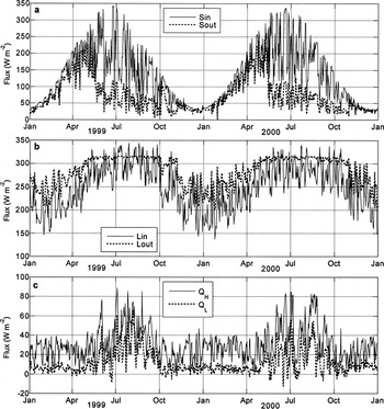
Fig. 11. Modelled daily mean fluxes of incoming and reflected shortwave radiation (a) incoming and outgoing longwave radiation (b) and latent- and sensible-heat fluxes (c) at M1 for 1999 and 2000.
For M1, Figure 12 shows the energy fluxes averaged over the year 1999 and over the time when there was melting. Similarly, mean fluxes were calculated for two other locations on the glacier: Msun and Mshad. Both are located at 2697 m a.s.l. However, Msun slopes to the west (about 7°) and Mshad steeply to the north (about 38°). Consequently, Mshad is shaded between sunrise and sunset for 74% of the year. For Msun, this is 23%, and for M1 44%. The mean surface energy flux of the melting period equals the energy involved in melting. At M1, melting occurs for 31 % of the year, and at Msun and Mshad the surface melts for 22% and 19% of the year, respectively. At all locations, the energy fluxes increase when the glacier melts. The longwave heat fluxes are generally the greatest fluxes, although incoming shortwave radiation is the largest flux at Msun during the melt period. The large difference between melt at Msun and Mshad is explained by the difference in shortwave radiation due to the topography at the two locations. Therefore, the specific mass balance at Msun (−2.50 m w.e.) is 2.7 times larger than at Mshad (−0.93 m w.e.). At M1, the specific mass balance is −5.78 m w.e. The turbulent heat fluxes are small at all locations, but supply 34% of the energy involved in the melting at M1, 23% at Msun and 40% at Mshad.

Fig. 12. Simulated energy fluxes averaged over the year 1999, and over the period when the surface was melting for three locations on the glacier (see text): M1 (a), Msun (b) and Mshad (c). All fluxes are positive towards the surface, except Sout and L out.
6.5. Climate sensitivity
Simple climate-sensitivity tests have been carried out for Morteratschgletscher. We altered the air temperature by 1°C and precipitation by 10% and recalculated the mean specific mass balance for 1999. Table 5 shows the results.
Table 5. Change in the mean specific mass balance (ΔB in m w.e.) in 1999 with respect to annual changes in air temperature (T) and precipitation (P)

The temperature sensitivities are larger than those for Hintereisferner, Austria, and Rhonegletscher, Switzerland, as computed by Reference OerlemansOerlemans (2000b, Reference Oerlemans2001). He found a change in the mean specific mass balance of −0.41 m w.e. for a 1°C temperature perturbation for both Rhonegletscher and Hintereisferner. For Pasterzenkees, Reference Greuell and BöhmGreuell and Böhm (1998) computed a much larger change in the specific mass balance for a 1°C warming: −0.90 m w.e. The change in the specific mass balance to a perturbation in precipitation is similar to the precipitation sensitivity of Hintereisferner (0.28 m w.e.) and Rhonegletscher (0.26 m w.e.) as determined by Reference OerlemansOerlemans (2000b, Reference Oerlemans2001).
The results reveal that increasing precipitation affects the mean specific mass balance of the glacier directly and indirectly. Without a perturbation, the mean snowfall on the glacier in 1999 is 1.26 m w.e. Therefore, a 10% change in precipitation explains only part of the change in the mean specific mass balance of about 0.18 m w.e. The remaining part is explained by the albedo feedback. Changing the air temperature affects mainly the incoming and outgoing longwave radiation and the turbulent heat fluxes, enhanced by the albedo feedback mechanism. According to Reference Greuell and BöhmGreuell and Böhm (1998), the albedo feedback causes roughly a doubling of the climate sensitivity.
7. Concluding Remarks
This research attempted to study the spatial distribution of the energy- and mass-balance fluxes of Morteratschgletscher, by using a two-dimensional mass-balance model. The ablation rate was calculated from the surface energy flux of the glacier. Meteorological data from four synoptic weather stations served as input for the model. Since Morteratschgletscher is located between high mountains, we corrected shortwave radiation for shading, aspect, slope, reflection from the slopes, and obstruction of the sky. We derived the albedo from snow depth and snow age, by following Reference Oerlemans and KnapOerlemans and Knap (1998). We used a method of Reference Oerlemans and GrisogonoOerlemans and Grisogono (2002) to calculate the turbulent heat fluxes within the glacier boundary layer. The model was run for two model years.
The comparisons of model results with observations from automatic weather stations located on Morteratschgletscher suggest that the model performs well. The residual standard deviation between calculated and observed daily radiation fluxes is < 22 W m−2. Modelled and measured snow accumulation reveal discrepancies. However, optimizing the snow-accumulation parameterization scheme is difficult because the spatial distribution of snow accumulation is hard to measure. The observed specific mass balances measured with stakes and a sonic ranger at three locations appear to exceed the mass balances modelled for the grid-cells in which the stations were located. The slope of the surface explains this to a large extent, because the stations are placed on relatively horizontal surfaces, whereas the gridcells are inclined towards the north.
In the future, the albedo scheme of the model should be improved, because the parameterization used was derived from a 1 year record measured at M1 by Reference Oerlemans and KnapOerlemans and Knap (1998). It is likely that the albedo parameters differ with elevation since the amount of debris on the glacier appears to decrease with elevation. The albedo of Morteratschgletscher will be investigated in more detail by using satellite data.
Then, modelled turbulent heat fluxes should be compared to measurements. It would be useful to observe the turbulent heat fluxes by eddy correlation measurements over a longer period of time in order to test the model of Reference Oerlemans and GrisogonoOerlemans and Grisogono (2002) and to determine a value for C b explicitly.
The parameter sensitivity test showed that uncertainty in the fractional cloud cover significantly influences the modelled mass balance. Consequently, an improved method of estimating the fractional cloud cover is desirable.
The model is useful for investigating the spatial pattern of the energy- and mass-balance fluxes. The fluxes vary mainly with elevation, but shortwave radiation, especially, also varies along the contour lines and supplies most of the melting energy. The results show that the mean shortwave radiation on the glacier would be 37% larger if the effects of the topography were discounted. This would lead to a decrease of 0.34 m w.e. in the mean specific mass balance of Morteratschgletscher. We conclude that it is important for mass-balance modelling to take into account the topographic effects on shortwave radiation. The mean specific mass balance changes about 0.67 m w.e. if the free-atmospheric air temperature differs by 1°C, and 0.17 mm w.e. if precipitation changes by 10%.
In the future, this mass-balance model will be used for several purposes. Firstly, results of the spatially distributed mass-balance model will be compared to results of a one-dimensional mass-balance scheme in order to improve the performance of a one-dimensional model. Then the sensitivity of the specific mass balance to climate changes will be studied in more detail. Lastly, a mass-balance reconstruction of Morteratschgletscher will be generated from historical meteorological records.
Acknowledgements
We would like to thank the people of the Ice and Climate Group of the IMAU, the reviewers, G. Wendler and R. Hock, and the Scientific Editor, R. Naruse, for numerous helpful comments made on the original draft of this paper. We are grateful to A. Souren for improving the English, and Meteo Schweiz for providing the meteorological data.


