3.1. The three Landsat images and their pre-processing

Three Landsat images, with a 30 m pixel size, are used to determine surface velocities (see Table 1). The main velocity field is inferred from a pair of Landsat 7 Enhanced Thematic Mapper Plus (ETM +) images acquired 21.5 months apart: on 26 February 2000 and 13 December 2001. Thus, the main velocity field can be regarded as a 2 year velocity mean centered in mid-January 2001. The last scene, available from the Landsat 5 Thematic Mapper (TM), was acquired 2 January 1989. Correlated with the 2000 image, it gives us the 11 year mean velocity of the ice stream centered in late July 1994. Comparison of the two sets of velocity data could help to detect possible changes of Mertz Glacier over the last decade.

Table 1. Landsat images used to study Mertz Glacier

The images are pre-processed to remove the noise and to enhance the small ice features (mostly crevasses) known to move with the flow (Reference Lucchitta and FergusonLucchitta and Ferguson,1986). First, we compute the first principal component of the visible and the near-infrared bands. This step yields low-noise images and enhances the topography. Scan-line striping was removed from the 1989 image using a destriping algorithm, described in Reference CrippenCrippen (1989). A spatial filter is then applied to create two sets of images: the low-pass filtered set is used for the co-registration, the high-pass filtered set for the determination of the displacements. The scale of the filter is chosen to separate the small-scale features, moving with the flow, from the fixed long-wavelength features due to the response of ice flowing over topographic features of the bedrock (Reference PatersonPaterson, 1994). This is obtained with a scale of the filter roughly equal to the ice thickness (Reference Budd and CarterBudd and Carter, 1971), about 1 km in the case of Mertz Glacier.

The co-registration of the images is one of the key points of the pre-processing because it will affect the accuracy of the velocities, especially when the time separation is short. First, “visual” co-registration is performed, shifting one of the two images with an offset deduced from comparing the bedrock features in each pair of images.Then, a cross-correlation method (described below) is applied between each low-pass filtered pair. The largest windows are used for this correlation to encompass the maximum of the low-frequency undulations. Using this methodology, Reference Scambos, Dutkiewicz, Wilson and BindschadlerScambos and others (1992) assumed an accuracy of ±1 pixel for the co-registration. Our results (mostly the standard deviation) indicate that a ±2 pixels accuracy is more reasonable in our study. If P _s is the pixel size (30 m) and Δt the time separation between the two images, this leads to an error for the velocities of 2P _s/Δt. This error is referred to below as the “systematic error” and noted . It equals ±33 m a⁻¹ for the 2000–2001 pair and ±5 m a⁻¹ for the 1989–2000 pair.

3.2. Determination of the velocity field

A complete description of the methodology followed to generate the velocity field is found in Reference Scambos, Dutkiewicz, Wilson and BindschadlerScambos and others (1992). Briefly, two high-pass filtered images are used to track the motion of small features by cross-correlating their brightness pattern. Generally, a 32 × 32 pixel area is used as a correlation window, but it is changed to 16 × 16 when tracking sharp features or to 64 × 64 for larger, diffuse ones. The cross-correlation algorithm determines the displacement of the features to sub-pixel precision as well as the strength of the correlation and an estimation of the error in the displacement. The displacement is then assigned to the center of the segment linking the two successive positions of the moving feature.

For the 2000–2001 pair, the 21.5 month time separation results in very little change in surface features and reasonable displacements. Even in the fastest part of the ice stream, the maximum displacement is 60 pixels. Thus, features do not show strong deformation and are easy to track.The accuracy of the cross-correlation is estimated to be ±0.5 pixel for this pair, which corresponds to ±8 m a⁻¹.This error, inherent in the cross-correlation, is referred to below as the “random error” and noted . Computed using Equation (4), the rand total uncertainty for the 2000–2001 velocities reaches:

(1)

Note that the uncertainty is independent of the absolute value of the velocity. The relative error would be 100% in an area moving at 34 m a⁻¹, and only 3.4% if the ice speed reaches 1000 m a⁻¹.

For the 1989–2000 pair, the situation is more complicated because of the 11 year time separation. Displacements are much larger, reaching 350 pixels in the center of the ice stream. Moreover, changes due to the wind modification of features and strong distortion of the crevasses make them difficult to track either visually or with the cross-correlation algorithm. In this case, the accuracy is estimated to be around ±2 pixels for the displacements. Due to the long time separation, the precision of the velocities remains high: the total uncertainty for the 1989–2000 velocity equals ±8 m a⁻¹.

4.1. Velocity field of Mertz Glacier

The main velocity field is obtained from the 2000–2001 pair, and a contour map is shown in Figure 2. More than 16 700 velocity points were used to produce this map. Each of these velocity points results from the cross-correlation algorithm. Automatic selection criteria remove the matches with low correlation strength or large errors. A vector median filter is also applied to remove inconsistent vectors in regions of high density of velocity points (Reference Astola, Haavisto and YrjöAstola and others, 1990). Eventually, each match is reviewed visually on the computer screen. The contour map is then produced in two steps. Velocity points are resampled to a 2 km grid, keeping in each gridcell a mean velocity value at the mean location of all the velocity points inside the cell. Then a surface is fitted to all these values using a 1 km grid size. This velocity dataset is available at http://nsidc.org/data/velmap/.

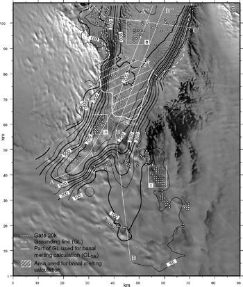
Fig. 2. Contour map of the velocity field of Mertz Glacier deduced from the 2000–2001 pair of images. Contours are drawn every 100 m a⁻¹ except for the 50 m a⁻¹ contour. Contours are plotted only where velocity data are available. White circles represent the velocity points deduced from the 1989–2000 pair of images. Ice flows from the lower part to the upper part of the map.White lines locate the three velocity profiles of Figure 3, white boxes (labeled a, b and c) the subscenes detailed in Figure 4.The grounding line (GL) and the gate 20 km downstream (20k) are also plotted.

To better represent the ice-velocity gradients and the shear on the margin of the ice stream, two longitudinal profiles (panels a and b) and one transversal profile (panel c) are shown in Figure 3. To encompass enough velocity points, these profiles are created from the projection of all the velocity measurements within a certain distance of the profile. The swath of the projection must be wide enough to include numerous velocity points and narrow enough to represent well the region where the velocity gradient is high. A width of 100 pixels, i.e. 3 km, is found to be a good compromise. Also in Figure 3, for the 2000–2001 pair, we added the velocities (solid line) and their error envelopes (dotted line) extracted from a high-resolution gridded velocity field.

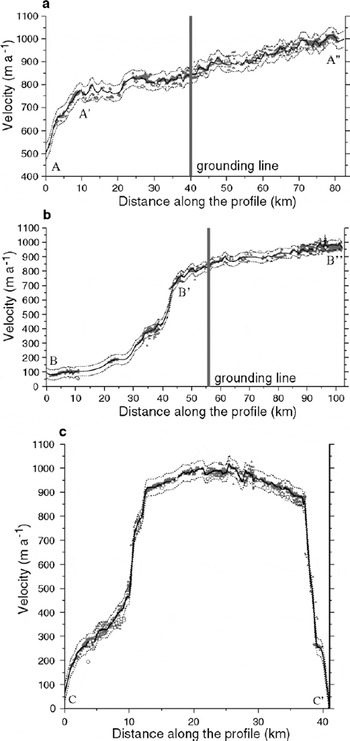
Fig. 3. Longitudinal and transverse velocity profiles of the ice stream: (a) along the main tributary; (b) along the secondary tributary; (c) transverse in the downstream part of the ice stream. The gray triangles represent velocity measurements from the 2000–2001 pair, the white circles measurements from the 1989–2000 pair. The black line represents the gridded velocity for the 2000–2001 pair, and the dotted lines the error envelopes obtained by adding and subtracting the uncertainty (34 m a⁻¹).

In Figures 2 and 3, we plot the grounding line determined by Reference RignotRignot (2002) using tidal movement of the tongue as visible with InSAR. Using an original combination of interferograms from the descending pass, Reference Pötzsch, Legrésy, Korth and DietrichPötzsch and others (2000) also located the grounding line of Mertz Glacier. The two maps are consistent even if some differences exist. In Figure 2, we located the gate 20 km downstream of the grounding line (labeled “20k”) used to calculate basal melting.

Velocities range from a few m a⁻¹ to >1000 m a⁻¹. The contour map shows a well-defined main tributary feeding the ice stream from the lower left corner, i.e. southwest, of the map. In this main tributary, speed increases rapidly from 500 m a⁻¹ to 750 m a⁻¹ in 8 km (A to A′ in Fig. 3a). This velocity gradient is mainly due to an increase of the surface slope. In the new topography derived from multiple SAR interferograms by Reference Pötzsch, Legrésy, Korth and DietrichPötzsch and others (2000), it coincides with altitudes decreasing from 500 m to 100 m. Below this area, the speed increases still further from 750 m a⁻¹ to 1000 m a⁻¹ in 75 km.

Upstream mapping of the velocity in this main tributary is impossible due to a lack of trackable features. In these regions, where crevasses are absent, cross-correlation of optical imagery reaches its limit. Moreover, with our uncertainty of ±34 m a⁻¹, velocity measurements in the catchment area would be highly uncertain.

This southwestern location of the main tributary is in agreement with the catchment area derived from topographic data by Reference RignotRignot (2002). The drainage basin is mostly located in the western and southwestern part of the ice stream (Fig. 1). In the eastern and southern parts, the ice is drained by the Ninnis Glacier system, the neighboring ice stream to the east.

The velocity map also highlights a second tributary located east of the first one. A longitudinal profile along the tributary (B−B′ in Fig. 3b) also shows a great velocity increase when approaching the grounding line. In this zone, a few kilometers upstream from the grounding line, a 550 m a^{− 1} velocity increase is observed in only 17 km. Note that these velocity gradients (and consequently the strain rate determined below) have small errors because they result from relative differences in velocity: the systematic error due to the misfit in the co-registration vanishes; only the random error inherent in the automatic feature tracking remains.

4.2. Comparison with the 1989–2000 velocities

The second pair of images (1989 and 2000) does not produce a complete velocity field: surface features were greatly deformed, so matches are sparse and many of them unreliable. A total of 433 displacement vectors is obtained: not enough to create a reasonable velocity contour map for the whole ice stream. However, in a few regions where the density and quality of the matches are good enough, we can make a comparison with the 2000–2001 velocities. Given the uncertainty in the two datasets, a change in velocity is significant if greater than i.e. 35 m a⁻¹. Thus, even for the fastest part of the glacier the change in velocity must be >3.5% to be detectable.

On the longitudinal profile A−A′−A″ and the transverse profile C−C′ in Figure 3, we observe that most of the 1989– 2000 velocity points are similar in magnitude to the slowest points for the 2000–2001 pair but not different enough to conclude that a major change in the flow speed occurred. Our plot of the velocity profile, i.e. a projection of all the velocity points within a certain distance of the profile, affects the quality of the comparison. It artificially creates a noise in the velocity due to the spatial variation of the velocity within this distance.

Comparing directly the velocities in a few regions is more precise: three regions are located in Figure 2 and are shown in more detail in Figure 4. On these regions, we plotted the velocity contours for the 2000–2001 pair and wrote the velocity values obtained from the 1989–2000 pair. For the two subscenes located along the main flow (Fig. 4a and b), a consistent velocity change of 30 m a⁻¹ is observed. This change is under our sensitivity limit of about 35 m a⁻¹. However, when looking at the third subscene located in a region of slow-moving ice (Fig. 4c), we can see that this sensitivity limit may be overestimated: the two sets of velocities are in good agreement and differ only by 10 m a⁻¹ in the worst case. This observation holds for all the slow-moving areas. Thus, the 35 m a⁻¹ value (proved above to be independent of the speed) is quite conservative.

Fig. 4. Three regions of the ice stream (a–c; see Fig. 2 for locations) where enough matches for the old pair of images (1989–2000, white circles) allow a significant comparison with the velocity contours from the recent pair (2000–2001).The two first subscenes (a, b), along the main tributary, show an increase in velocity of around 30 m a⁻¹; the third (c), in a slow-moving part of the glacier, shows no change in velocity.

We calculated the mean difference between the two sets of velocities. Where measurements are available for the oldest pair, we extracted from the gridded dataset the velocities for the 2000–2001 pair. The mean velocity increase reaches 15 m a⁻¹, but the standard deviation (rms) of this difference (45 m a⁻¹) reflects its large spatial variability and the uncertainties.

The Mertz ice stream may have experienced a slight increase in speed during the last decade, but we cannot prove it, so we conclude that the flow of Mertz Glacier is stationary within our uncertainty. The main limitation is the lack of velocity measurements for the old pair, which prevents us from carrying out a statistical study. A velocity change, if existing, could be better detected with a supplementary image from 1991 or 1992. Thus, we would produce a complete velocity field for the early 1990s and increase the time separation between the two pairs.

4.3. Strain rate of the ice stream

In section 4.1, we touched on the topic of longitudinal strain rate. A velocity increase of 250 m a⁻¹ in 8 km along the main flow is similar to a longitudinal strain rate of 0.03 a⁻¹. This value is in good agreement with the longitudinal strain-rate map (Fig. 5a). This map was produced using the method described in Reference NyeNye (1959). This calculation includes a rotation to a local coordinate system parallel (x axis) and perpendicular (y axis) to the flow direction. Starting from a 1 km gridded velocity field, we calculated the longitudinal, transverse and shear strain rates using the equations shown in the appendix of Reference Bindschadler, Vornberger, Blankenship, Scambos and JacobelBindschadler and others (1996). These results were then resampled to a 6 km grid, a scale which proved to be a good compromise between enhancing the signal-tonoise ratio (by filtering the small-scale dynamics effect) and preserving the significant spatial features.

Fig. 5. Strain-rate maps of Mertz Glacier deduced from the 2000–2001 velocity field: (a) the longitudinal strain rate and (b) the shear strain rate.

The longitudinal strain-rate map (Fig. 5a) underscores the two main tributaries of the ice stream where a significant increase in velocity creates a positive strain rate (>0.03 a⁻¹), i.e. a horizontal stretching. An increase in the density of crevasses with a direction perpendicular to the flow can be observed in these regions. Between the two tributaries a region of negative longitudinal strain rate reflects the effects of a probable obstruction feature in the bedrock. The flow slows down and compression appears upstream of this feature. After crossing the grounding line, the central part of the ice stream experiences lower longitudinal strain rate than the margins. For the whole ice stream, a positive mean longitudinal strain rate (0.6 × 10⁻³ a⁻¹) shows that a horizontal stretching regime prevails.The margins are affected by a large shear strain rate exceeding 0.04 a⁻¹ (Fig. 5b). The ice stream is divided into two symmetric regions affected by a shear of similar amplitude but opposite signs. This pattern underscores the highly symmetric flow in Mertz Glacier. The transverse strain rate (not shown here) is generally opposite in sign to the longitudinal strain rate.

The vertical strain rate, , can be obtained from mass continuity if density is constant:

(2)

where and are the longitudinal and transverse strain rates. The values of the vertical strain rate are mainly negative. A mean value of −0.7 × 10⁻³ a⁻¹ for the whole grounded ice stream is the result of the thinning of the ice while flowing to the sea (Reference Bindschadler, Vornberger, Blankenship, Scambos and JacobelBindschadler and others, 1996).

5.1. Discharge fluxes

Obtaining accurate and well-distributed velocity measurements allows the calculation of the discharge fluxes of the ice stream at different “gates” transverse to the flow and crossing the whole ice stream. Each gate is broken into a number of small segments or “individual gates”, through each of which the discharge flux is calculated and summed. The number of gates must be high enough to take into account each change in the magnitude or the direction of the velocity. The mass flux through a given gate,Φ_gate, is calculated according to:

(3)

where v _⊥i is the velocity component perpendicular to the ith segment, H_i the mean ice thickness of the ith segment, and δw_i the width of the ith segment.

For the ice thickness, due to the lack of reliable data in the region of Mertz Glacier (the BEDMAP database includes only three points over the Mertz Glacier tongue), we used the assumption proposed by Reference RignotRignot (2002) of hydrostatic equilibrium of the floating part of the ice stream. Following Reference RignotRignot (2002), the ice thickness is deduced from the European Remote-sensing Satellite (ERS) digital elevation model (DEM) by multiplying the elevation by 8.05.This factor includes both the hydrostatic equilibrium of ice floating over sea water and an offset in geoidal height. Restricted to this assumption, we were only able to calculate discharge fluxes downstream of the grounding line. According to Reference RignotRignot (2002), the uncertainty of these estimates of ice thickness, σ_H , can be considered as a constant equal to 100 m.

Another key assumption in Equation (3) is constant velocity with depth. Reference Bindschadler, Vornberger, Blankenship, Scambos and JacobelBindschadler and others (1996) showed that this is already a good approximation for the grounded ice stream. For the floating ice, for which no basal drag is present, the bottom of the ice is a free surface and this assumption is all the more realistic.

At the grounding line of Mertz Glacier (noted GL in Fig. 2), we calculated an ice discharge flux of 17.8 km³ a⁻¹.

The uncertainty of this value has to be calculated carefully. As detailed previously, the uncertainty for the main velocity field, is 34 m a⁻¹.This is also the uncertainty of the velocity perpendicular to each segment: in the worst case, this velocity error will be perpendicular to the segment. We assume that the uncertainty of the width of each gate is negligible, supposing that the pixel size of 30 m provided by Landsat is accurate. The uncertainty is calculated using the following formula extracted from Reference BevingtonBevington (1969). If Φ is our final result, composed of a functional relation f between independent parameters x, y, z, … and if σ_x , σ_y , σ_z , … are the uncertainties in x, y, z, … and are uncorrelated, then the uncertainty in Φ is:

(4)

Applying this equation to the discharge fluxes leads to an uncertainty of:

(5)

The uncertainty of the ice discharge flux at the grounding line is 1.2 km³ a⁻¹ and is equally due to the uncertainty of the velocity and of the ice thickness.

5.2. Basal melting

As proposed by Reference RignotRignot (1996), the melting at the base of the floating part of the ice stream can be calculated by using at least two transverse gates. To calculate the basal melting of Mertz Glacier, we used a closed contour including part of the grounding line and another gate located 20 km downstream (noted and 20k respectively in Fig. 2). The area delimited by this contour is 375 km2. The basal melting is calculated by:

(6)

Where is the discharge flux (m³ a⁻¹ of ice) at (part of) the grounding line,Φ_20k the discharge flux (m³ a⁻¹ of ice) 20 km downstream of the grounding line, the area (m²) between the two gates, and the accumulation rate (m a⁻¹ of ice) between the two gates.

Note the difference between and Φ_GL:Φ_GL is the discharge flux through the whole grounding line, whereas is the discharge flux through the part of the grounding line forming a closed contour with the gate 20 km down-stream (see Fig. 2 to visualize this difference). Thus, .

With and Φ_20k = 12.6 ± 0.9 km³ a⁻¹ of ice, and an accumulation rate around 0.35 m a⁻¹ of ice (Reference Vaughan, Bamber, Giovinetto, Russell and CooperVaughan and others, 1999), we estimate the basal melting to be 11 m a⁻¹ of ice.

Assuming no error in and an accumulation accurate at ±0.1 m a⁻¹ , the uncertainty of the basal melting is:

(7)

We estimate to be ±4 m a⁻¹ of ice.

Our basal-melting estimate of 11 m a⁻¹ of ice is nearly 40% lower than the value of 18 m a⁻¹ of ice calculated by Reference RignotRignot (2002). This difference is mostly due to our slower flow speed when crossing the grounding line: at the grounding line, the difference between our ice discharge flux (16.6 ± 1.1 km³ a⁻¹) and that from Reference RignotRignot (2002) (19.8 ± 2 km³ a⁻¹) 3.2 km³ a⁻¹, whereas it is only 0.5 km³ a⁻¹ at the gate 20 km downstream (12.6 ± 0.9 vs 13.1 ± 1 km³ a⁻¹). We demonstrated previously that the flow of Mertz Glacier is nearly constant, and thus we attribute these differences to errors in the velocities of Reference RignotRignot (2002). These errors could be due to the fact that “both [Ninnis and Mertz] glaciers flow nearly parallel to the satellite track direction” (Reference RignotRignot, 2002) which affects the accuracy of the InSAR measurement of the ice velocities. Still, basal melting remains the main factor of ablation for the Mertz Glacier tongue. Due to the limited northern extension of the Landsat scenes we used, the calculation could not be extended in the seaward part of the tongue. Our value for the basal melting is only representative of the first kilometers of the Mertz Glacier tongue. Reference Frezzotti, Tabacco and ZirizzottiFrezzotti and others (2000), studying outlet glaciers from the Dome C area, showed that basal melting (and freezing rate) can significantly change along the floating tongue.

5.3. Mass balance

The mass balance of the drainage basin can then be estimated using the mass budget method as detailed in Reference RignotRignot (2002). The total input was calculated by Reference RignotRignot (2002). Using a DEM of Antarctica, the Mertz drainage basin is delimited and has an area of 83 080 km². On this area, the digital accumulation maps of Reference Vaughan, Bamber, Giovinetto, Russell and CooperVaughan and others (1999) and Reference Giovinetto and ZwallyGiovinetto and Zwally (2000) are integrated to estimate the total annual accumulation: 21.3 km³ a⁻¹ of ice. The mean accumulation for the whole catchment area is thus 256 mm a⁻¹ of ice. This is less than the 272 mm a⁻¹ of ice previously proposed byReference Wendler, Ahln s and LingleWendler and others (1996).

Thus, Mertz Glacier seems not to be in balance, with an annual input 3.5 km³ of ice higher than the output. If existing, such an imbalance would result in a rate of ice thickening of 4.2 cm a⁻¹ over the catchment area. Using altimeter data from Seasat and ERS-1, Reference Rémy and LegrésyRémy and Legrésy (1998) mapped the changes in the height of the Antarctic ice sheet between 1978 and 1992. The only area showing a significant rise of the surface is located at 70–72° S,140–150° E and includes part of the Mertz drainage basin. The rise (20–25% of the accumulation rate) is not very different from our imbalance of 3.5 km³ of ice, which represents 16.5% of the accumulation rate on the Mertz drainage basin.

On the other hand, the map proposed by Reference Wingham, Ridout, Scharroo, Arthern and ShumWingham and others (1998) does not show any significant elevation change in the catchment area of Mertz Glacier. We are quite confident in our estimation of the velocity at the grounding line. More uncertainties remain in the ice thickness which results from an assumption. We also wonder whether the accumulation rate on the drainage basin is accurate in an area subject to the strongest wind in the world (Reference Wendler, André, Pettré, Gosink, Parish, Bromwich and StearnsWendler and others, 1993) and where blue-ice areas are widespread. In the accumulation-rate map of Reference Vaughan, Bamber, Giovinetto, Russell and CooperVaughan and others (1999), these are assumed to be areas of nil accumulation although they undergo ablation. Despite the assertion by Reference Bintanja and van den BroekeBintanja and Van den Broeke (1995) that blue-ice areas are “too small to play an important role in the total surface mass balance regime in Antarctica”, we believe that, in some catchments such as Mertz, they could be significant. Another uncertainty results from the very coarse grid in the accumulation-rate map of Reference Vaughan, Bamber, Giovinetto, Russell and CooperVaughan and others (1999): the grid spacing of 1 is probably too coarse to represent the steep gradient in precipitation near the coast. We suspect that the export of snow by wind (Reference LoeweLoewe, 1972) is not well taken into account in the accumulation map. The low density of measurements used by Reference Vaughan, Bamber, Giovinetto, Russell and CooperVaughan and others (1999) in the Mertz area could affect the extrapolation process to a gridded dataset of accumulation: the extrapolation of points with less wind erosion to areas of much greater wind erosion (such as the grounding line of Mertz Glacier) could lead to an overestimation of the accumulation rate in those windy areas. If we assume no imbalance for Mertz Glacier, our measurements suggest that the wind could export 16.5% of the total precipitation on the drainage basin. This is close to the value of 15% proposed byReference Wendler, Ahln s and LingleWendler and others (1996). Blowing winds not only export snow: they also increase sublimation. Reference BintanjaBintanja (1998) quantified this effect using a one-dimensional atmospheric surface layer model based on observations from automatic weather stations on a transect from Dumont d’Urville to Dome C. Extrapolated to the whole of East Antarctica, the model shows that snowdrift sublimation removes 19 mm a⁻¹ of ice. This represents 7.5% of the total precipitation on the Mertz drainage basin.