


1. INTRODUCTION
Ice cores retrieved from high-latitude regions are an important archive of past climate (Taylor and others, Reference Taylor2005; Brook and others, Reference Brook, Wolff, Dahl-Jensen, Fischer and Steig2006). Deep ice core drilling has provided climate reconstructions reaching back almost one million years (Wolff and others, Reference Wolff2010), including records for air and sea surface temperature, atmospheric circulation patterns, atmospheric concentrations of pollutants, dust and greenhouse gases (Ahn and others, Reference Ahn2004; EPICA Community Members, 2004; North Greenland Ice Core Project members, 2004; Wais Divide Project Members, 2013).
All intermediate-depth and deep cores face the challenge of ‘brittle ice’ (Gow, Reference Gow1968; Gow, Reference Gow1971), generally occurring at a depth of 500–1100 m from the surface (Neff, Reference Neff2014). At these depths, the overburden of pressure on air bubbles trapped in the ice leads to rapid decompression once the ice is brought to the surface and is exposed to ambient air pressure (Uchida and others, Reference Uchida1994; Taylor and others, Reference Taylor2005). The ice sometimes violently explodes on the core extraction table, but more often simply acquires breaks and microfractures inside the core (Gow, Reference Gow1971). Fractured pieces usually need to be removed in their entirety before analysis to create a clean, flat surface and prevent contamination, potentially representing a loss of important climate history. This problem is particularly acute for intermediate-depth high-accumulation coastal sites like Roosevelt Island in Antarctica, where the brittle ice can make up 50% or more of the length of the ice core and may represent many thousands of years and as much as 90% of the pre-Holocene climate history (Neff, Reference Neff2014).
Ice from the brittle ice zone (BIZ) is vulnerable throughout handling and processing, with potential to introduce more breakage and to further degrade the quality of the ice (Neff, Reference Neff2014; Souney and others, Reference Souney2014). Certain measures can be taken to minimize fractures, such as modified drilling techniques, storing the ice before shipping and ‘relaxing’ the ice (letting it rest and slowly decompress) for several months or years after drilling and prior to cutting and analysis (Gow, Reference Gow1971; Neff, Reference Neff2014). Despite these efforts, almost all intermediate and deep ice cores suffer from some degradation in quality in the BIZ (Neff, Reference Neff2014; Souney and others, Reference Souney2014). Thus, it is important to develop techniques to improve the processing and analyses of brittle ice.
Continuous flow analysis (CFA) is a common method used to analyze ice cores for isotopic ratios, gases and chemical content (Osterberg and others, Reference Osterberg, Handley, Sneed, Mayewski and Kreutz2006; Kaufmann and others, Reference Kaufmann2008). CFA systems usually consist of a melt head connected to multiple analytical instruments, with one end of the ice core placed on a heated plate and melted at a controlled rate, generating a continuous stream of meltwater, gases and particles that is then divided and fed to instruments for real-time measurement. However, brittle ice presents a technical challenge for CFA (Osterberg and others, Reference Osterberg, Handley, Sneed, Mayewski and Kreutz2006; Bigler and others, Reference Bigler2011), as poor-quality ice and fractures or breakages can introduce contaminants such as drilling fluid, create discontinuities in the data (Neff, Reference Neff2014) or otherwise compromise the quality and precision of the measurements (Bigler and others, Reference Bigler2011). CFA systems have achieved increasingly high precision and quality in recent years (Bigler and others, Reference Bigler2011; Chappellaz and others, Reference Chappellaz2013; Emanuelsson and others, Reference Emanuelsson, Baisden, Bertler, Keller and Gkinis2015; Jones and others, Reference Jones2017). However, the degree of precision and/or resolution depends not only on the measurement technique but also on the quality of the ice. In the majority of cases, brittle ice is too fragmented and/or fragile to be analyzed via CFA systems.
In this paper, we focus on (a) our drilling system, designed to minimize fractures at the time of core recovery, and (b) a novel approach used to process the ice from the Roosevelt Island Climate Evolution (RICE) ice core, which allowed us to successfully conduct CFA water-stable isotope measurements on 94.2% of the total length of the core, including 87.8% of the BIZ. We present a method to conserve brittle ice for CFA by melting non-horizontal fractures, i.e. breaks that occur on an angle (‘slanted breaks’).
In the following sections, we outline the steps taken to maintain the integrity of the brittle ice prior to measurement, the modifications to procedures and CFA setup to accommodate slanted breaks, and an analysis of the effects of slanted breaks on the quality of the water-stable isotope data from the RICE core below 500 m depth. We conclude with recommendations for future ice core drilling and processing campaigns.
2. METHODS
2.1. RICE site, drilling and core storage
RICE is an international collaboration that drilled and retrieved a 764 m-long ice core from the north-eastern edge of the Ross Ice Shelf on Roosevelt Island in Antarctica (79.39S, 161.46W, 550 m a.s.l.) during two austral summer field seasons, 2011–2012 and 2012–2013. Roosevelt Island is a high snow accumulation site (Bertler and others, Reference Bertler2018) with the potential for a highly resolved record. The RICE BIZ occurs from 500 m depth to bedrock, which was reached at 764 m. This part of the core contained a higher number of fractures, representing a potentially significant loss of ice for CFA. Overall, 87% of the dated climate history in the RICE record is captured in the BIZ, which represents 35% of the entire core depth, underscoring the need to preserve as much brittle ice as possible for CFA.
Several techniques were employed in the field to preserve the integrity of the brittle ice before processing or measurement took place. The design of the New Zealand ice coring drill (Te Wāmua Hukapapa or ‘Ice Cores That Discover the Past’ in the NZ Te Reo native language), based on the successful Danish Hans Tausen Drill design (Johnsen and others, Reference Johnsen2007), was crucial in keeping the fractures in the core to a minimum. In particular, a hydraulic-powered aluminum box section telescopic mast provided the core break force. The controllable tension applied by the hydraulic system to the cable drill and drill during core penetration and core breakage avoided subjecting the core to a sudden, strong and potentially destructive pull as it was lifted to the surface. In addition to the hydraulic system, the drill barrel length was modified to cut a 2 m-long core, and to add a longer perforated chips chamber (Popp and others, Reference Popp, Hansen, Sheldon and Panton2014) with a non-perforated hollow shaft with multiple spiral chip boosters (Mandeno and others, Reference Mandeno, Pyne, Bertler and Neff2013). An ‘off the shelf’ down hole logging winch with a four conductor ¼ inch diameter armored cable was used as the basis of the winch system. However, because the winch had insufficient pull for core breaks, which was expected to exceed 1000 kg force at times, the aforementioned hydraulic system was developed to provide the core break force and reduce the ‘roof’ height required of the drilling trench. The drill was operated in a trench cut into firn ice 3 m deep, 4 m wide and covered with a 22 m long bespoke aluminum-framed single skin ‘tunnel’ tent. The drill and drill trench are pictured in Figure 1.

Fig. 1. RICE drill trench and setup. Picture shows core curators measuring and cutting the core and drill operators cleaning and preparing the core barrel for the next core run. Labels refer to the following: (A) drill tent; (B) back entrance; (C) core processing table, where electrical conductivity measurements (ECM) are first made, and the cores are cut into 1 m pieces and weighed for density; (D) piece of ice ready to be weighed and bagged; (E) direction of the core buffer area and snow cave; (F) main entrance to drill trench; (G) geo mats cover the entire floor for stable footing; (H) drill controls for electro-mechanic drill and hydraulic mast; (I) drill fluid recovery tank; (J) chip spinner for drill fluid recovery.
These modifications taken together contributed to the high-quality core obtained throughout the drilling, especially during the recovery of the brittle ice. As shown in Figure 2 and Supplementary Table S1, most drill runs returned 2 m core sections in a single piece, with only 13 runs recovering core in three or more pieces, and only two of those runs recovering core in five pieces (representing the worst drill quality).

Fig. 2. For each drill run (designed to cut a 2 m length of ice core), number of pieces of ice recovered and brought to the surface vs accumulated depth. Most of the cores above 500 m depth were recovered in single 2 m lengths.
To ensure the integrity of planned measurements, particularly gases, ice cores need to be kept frozen at −18°C or colder (Ikeda-Fukazawa and others, Reference Ikeda-Fukazawa2005). Due to the relatively warm summertime temperatures at Roosevelt Island (Bertler and others, Reference Bertler2018), core curation in the field was an important challenge. Once the cores were drilled, they were kept in core rest buffer shelving (SF) to relax for up to 2 weeks. They were then cut into 1 m lengths and stored in the snow cave again, inside ice core boxes made of expanded polypropylene (SF). Photos and a schematic diagram of the core buffer and cooling system are in Supplementary Figures S1–S4.
During the first season, temperatures in the storage snow cave fluctuated between −23.4 and −13.3°C, and so an active cooling system was developed for the second season. A commercially available refrigeration system (Skope UF50AA) was modified to operate at low ambient temperatures; this included removing electronic thermostats and associated controllers and returning the unit to a more rudimentary electro-mechanical control system to ensure the refrigerator's robustness for Antarctic field operation. The refrigeration system otherwise maintained its basic core elements of compressor, expansion valve, evaporator and condenser (Mandeno and others, Reference Mandeno, Pyne, Bertler and Neff2013). The system kept the storage cave at −23°C or cooler despite ambient surface conditions reaching positive temperatures for short durations (hours) during the warmest part of the season in January. Further information on the refrigeration system can be found in the Supplementary Material.
After drilling concluded, the cores were flown to Scott Base, where they were stored in an ISO 20′ freezer container (RICE reefer) at −36°C. Supplementary Figure S5 shows an average temperature profile for an ice core box during field storage and the flight to and storage at Scott Base. At no point did the temperatures inside the box get warmer than −18°C. The reefer was then shipped to Christchurch, New Zealand, and trucked to the National Ice Core Research Facility in Lower Hutt, New Zealand, where the boxes were unloaded and kept at −36°C until the cores could be processed. The cores were cleaned and processed in the cold laboratory at −20°C over two periods in June/July 2013 (0–500 m) and April 2014 (500–761 m). The cores were then measured in two subsequent CFA melting campaigns during June/July 2013 and June/July 2014.
2.2. Core processing
2.2.1. Ice relaxation
There were relatively few fractures in the recovered ice at depths 0–500 m at the time of drilling (Fig. 2). Because of this, we were able to proceed with the analyses of this ice without further relaxation time and to cut only straight breaks in the ice prepared for CFA for the first melting campaign in 2013.
However, below 500 m, cutting the core with the horizontal and vertical bandsaws became problematic, causing additional fractures and spontaneous breakages. To attempt to reduce stress induced from the temperature difference between the cold laboratory (−20°C) where the ice was cut and the storage freezer (−36°C), the ice was brought into the cold laboratory 12 h prior to cutting. However, no observable improvement in the cutting performance was observed. In a second approach, the temperature of the cold laboratory was set to −28°C, but the ice became even more brittle and cutting performance further reduced. At this point, a decision was made to pause further cutting and relax the ice through longer term storage at −18°C. This temperature was deemed safe to ensure the integrity of the planned analysis (i.e. CO2 measurements, physical properties) but sufficiently warm to support gentle relaxation of the bubble pressure in the ice. After 8 months of relaxing (in April 2014), the ice was cut without inducing further fractures.
2.2.2. Core preparation for CFA
In the cold laboratory, the 1 m cores were divided into different cross-sections for analysis or archiving (see Supplementary Fig. S6). Either the ‘primary’ (A) or ‘secondary’ (B) section was selected for CFA, according to the number of breaks contained in the section and overall core quality (out of 761 sections melted, the ‘B’ section was chosen 109 times). The remaining section was held in reserve and melted if needed, in the event of equipment failure or otherwise poor results from the first section (this occurred only four times).
The 1 m core section was laid out on a bench top and cleaned. The first step in cleaning involved shaving 1–2 mm of exposed, potentially contaminated ice from the top and bottom of the section, thus creating a flat surface to fit two consecutive core sections together as closely as possible. This was done to avoid introducing ambient air during melting and contaminating the CFA methane record. Any other fractures or breakages in the middle of the section were also cut and cleaned in the same manner. Breaks were cleaned by hand using ceramic knives, although sometimes a drop-down saw was used in the first instance to achieve a well-fitted break. (For more information about the cleaning procedure, see the Supplementary Material.) A subjective decision was made in each case whether to cut a slanted or straight break based on which type would conserve the most material, considering the shape and angle of the existing fracture.
The total length of the core and the length and top and bottom location of the breaks (slanted or otherwise) were recorded to the millimeter (with ±1–2 mm error) both on paper and in an electronic spread sheet. An example is given in Supplementary Figure S7 and Table S2. This information was used to align each CFA data point with the corresponding depth in the core. For every break, the relative depth within the core was recorded at which the original break in the ice occurred, the length of the piece removed, and the position of the break after the edges had been cleaned and fitted back together. Slanted breaks required two additional pieces of information: the upper and lower depths of the pointed edges of the triangular wedges both before and after cutting (see Fig. 3). This allows us to determine precisely which parts of the data are affected by the smoothing over a slanted break.

Fig. 3. Diagram of core 498 B showing before cleaning (a) and after cleaning (b and c). (a) Shows the naturally occurring breaks before cleaning, which necessitated removing material from each colored section: green = 0.1 cm removed, blue = 0.5 cm removed, purple = 1.4 cm removed and peach = 0.2 cm removed. (b) Shows how the core was fitted together after cleaning and the position of each break. (c) Shows how the core would have looked after cleaning had we used the traditional method of cleaning for the slanted break (purple section) removing enough ice to create a straight break. In this instance, we would have lost an additional 7.8 cm of ice compared with the method that retained the slant feature. Colors correspond to the boxes with recorded break information in online Supplementary Fig. S7 and Table S2. Figure not drawn to scale.
2.3. Core holders
A key piece of equipment was the acrylic core holders, which were spring-loaded to keep the ice vertically in place over the melt head and to prevent misalignment of pieces during melting. As slanted pieces were more prone to misalignment and slippage, this was crucial to the quality of the analysis, keeping the ice centered on the melt head and preventing contamination from the outer ice. The core holders were modified from the University of Maine design (Osterberg and others, Reference Osterberg, Handley, Sneed, Mayewski and Kreutz2006). Specifically, the adjustable stabilizers were strengthened by adding an acrylic backbone and were coated in polytetrafluoroethylene to prevent the ice from sticking in the holders during melting. The backbone kept the slanted pieces from pushing the adjustable stabilizers apart. Extra springs were added to give better control and rigidity to the adjustable points. The original front door was also modified from one panel to three panels, each of which can be opened individually, which gave greater ability to manually adjust the position of the ice if necessary during melting (Supplementary Fig. S8).
2.4. CFA system
The RICE CFA system is a modified version of the Niels Bohr Institute setup (Bigler and others, Reference Bigler2011; Winstrup and others, Reference Winstrup2017). As with the system described in Bigler and others (Reference Bigler2011), it included a gold-coated copper melt plate that partitioned the inner and outer sections of the ice core and a debubbler to separate air and water from the inner aliquot. The inner portion of the core was directed through perfluoroalkoxy tubing (1/16″) from the melt head to various instruments for real-time continuous measurements of water-stable isotopes (Emanuelsson and others, Reference Emanuelsson, Baisden, Bertler, Keller and Gkinis2015), black carbon (Masiello, Reference Masiello2004; McConnell and others, Reference McConnell2007), methane (Stowasser and others, Reference Stowasser2012), calcium, insoluble dust particles (Bigler and others, Reference Bigler2011; M. F. Simonsen and others, unpublished information), conductivity (Bigler and others, Reference Bigler2011) and pH (Kjær and others, Reference Kjær2016). Drip counters collected inner water for discrete analyses of inductively coupled plasma mass spectrometry and ion chromatography (IC) measurements. In addition, meltwater from the outer portion of the core was collected in aliquots for discrete water-stable isotope and radioactive isotope analysis. A schematic of the CFA system is reproduced from Winstrup and others (Reference Wolff2017) in Figure S9 of the Supplementary Material. The system was controlled with an interface built with LabVIEW software (National Instruments). More details on the design of the CFA system are available in Winstrup and others (Reference Wolff2017).
The CFA setup for stable water isotope measurements (δ 2H, δ 18O) and a comparison to discrete measurements are described in detail in Emanuelsson and others, Reference Emanuelsson, Baisden, Bertler, Keller and Gkinis2015. We briefly review the most essential elements here. The water isotopes were measured using off-axis integrated cavity output laser absorption spectrometry (instrument manufactured by Los Gatos Research (LGR)) coupled to a commercially available Water Vapor Isotope Standard Source calibration unit (WVISS, manufactured by LGR) with a modified furnace and evaporation chamber (Emanuelsson and others, Reference Emanuelsson, Baisden, Bertler, Keller and Gkinis2015). The WVISS functioned as a sample introduction system: a nebulizer vaporized the liquid meltstream, which was then mixed with filtered, compressed dry air and delivered directly to the isotope water analyzer (IWA). The temporal resolution of the system is primarily determined by the time required to replace the volume of vapor in the WVISS evaporation chamber with new sample; to improve the response time, the volume of the chamber was reduced from the default 1.1 L to 40 mL. The 2013 and 2014 setups were the same except for a modification to the heating element of the vaporizer and a higher sample flow delivered directly to the IWA through an open split in 2014 (Emanuelsson and others, Reference Emanuelsson, Baisden, Bertler, Keller and Gkinis2015). The response time (defined as 5–95% of the total isotopic step change) was 54 s for the 2013 setup and 18 s for the 2014 setup (Emanuelsson and others, Reference Emanuelsson, Baisden, Bertler, Keller and Gkinis2015). This equates to ~3.0 and 1.0 cm depths, respectively. Data were sampled at a frequency of 2 Hz in 2013; however, since this exceeded the depth sampling resolution (1.0 mm), the frequency was reduced to 1 Hz in 2014.
2.5. CFA melting
Once cleaned and recorded, each segment of ice was carefully loaded into the core holders in preparation for melting. The core, in its holder, was placed upright in a freezer at −20°C, with one edge resting on top of the melt head. The melting plate was heated to 30°C and adjusted to keep the flow rate constant as the cumulative weight of the core reduced during melting. The melting rate was approximately constant at 3 cm min−1 over the course of the campaign, producing a liquid flow rate of ~16.8 mL min−1. Vertical displacement (or relative depth) was measured by an optical encoder as the core melted. Either three or four sequential 1 m segments were stacked on top of each other in the core holders and melted without interruption.
Calibration standards for water-stable isotopes were run between each stack. These calibrations were necessary to correct for instrumental drift and to monitor other measures of quality control (Emanuelsson and others, Reference Emanuelsson, Baisden, Bertler, Keller and Gkinis2015). Despite the interruption in measurement and potential data gaps, frequent calibrations are desirable, as the uncertainty introduced by drift increases with the amount of time from the nearest calibration (Keller and others, Reference Keller2018). Standards were introduced after the debubbler and after the line was split between IC, water isotopes and remaining CFA lines (see Supplementary Fig. S9). A multi-port valve (C25-3186EMH, VICI) was used to switch between the meltstream from the ice core and water standards for calibration. Immediately before and after each stack, we ran the Milli Q (18.2 MΩ) laboratory water standard, composed of local de-ionized water with an isotopic value (δ 18O = −5.89, δ 2H = −34.85) much greater than the RICE ice core. This created a transition period at the beginning and end of each stack where mixing occurs; the duration is determined by the response time of the instrument. We identified the portion of the data that was affected by mixing using a semi-automated algorithm and removed these points from the final dataset (Keller and others, Reference Keller2018). While this introduced data gaps of 2–5 cm every 3 or 4 m, this was necessary to ensure that the signal was not influenced by the finite response time and memory effects in the system.
During melting, the melting rate, the relative depth of the ice being melted and other system information was logged every second in a text file using LabVIEW software (National Instruments). Using the recorded depths, the slanted segments were identified and the depths were linearly scaled and expanded to fill the difference between the original piece of ice and the shortened piece with the cut removed. To obtain the expanded range of depths D′ = [D′1 … D′n] with minimum value D′1 and maximum value D′n, the following equation was applied to the original depth sequence D = [D 1… D n]:
 $${\bi D^{\prime}} = \; \left[ {\left( {{\bi D} - D_1} \right) \times \displaystyle{{D^{\prime}_n - D^{\prime}_1} \over {D_n - D_1}}} \right] + D^{\prime}_1. $$
This means that the CFA data over a slant cut represent a weighted average of two points of the core at different depths, introducing a linear mixing or smoothing into the data. We would thus expect the CFA data to have a reduced resolution proportional to the length of the break, but in most cases to still preserve a substantial portion of the original signal. As we demonstrate in the following section, the most noticeable effects will occur within the segments with rapid, small amplitude changes.
3. RESULTS AND ANALYSIS
We focus our discussion on the CFA water-stable isotope data from the RICE core because they are a fundamental part of any ice core study (Grootes and Stuiver, Reference Grootes and Stuiver1997; Legrand and Mayewski, Reference Legrand and Mayewski1997; Petit and others, Reference Petit1999; EPICA Community Members, 2004), and the detailed record obtained with the high resolution of laser spectroscopy (Emanuelsson and others, Reference Emanuelsson, Baisden, Bertler, Keller and Gkinis2015) allows us to more readily evaluate and detect subtle changes in the ice core quality. Examining the quality of other CFA measurements that were performed is beyond the scope of this paper; however, stable water isotopes are one of the highest resolution and most complete measurements in the RICE CFA campaign (with an 18 s response time in 2014), and thus the smoothing effect of including slanted segments in CFA is likely to be adequately represented in the stable isotope data. In general, the analysis outlined here can be applied to other types of CFA data.
3.1. Length and distribution of breaks
A total of 2.96 m of melted ice was part of a slanted segment. Thus, this method permitted us to continuously melt and analyze almost 3 m of ice (or 1% of the brittle ice) that otherwise would have been removed and only available for discrete analysis. On the age scale (Winstrup and others, Reference Wolff2017; Lee and others, in prep), this represents ~1300 years of climate record. Within the BIZ, the bottom 261 m of the RICE record, a total of 31.8 m (or 12.2%) of ice was removed from the CFA material due to cleaning of core ends and fractures (including both straight and slanted breaks). Hence, 87.8% of the brittle ice was melted for CFA measurements.
The distribution of both straight and slanted breaks is weighted toward deeper segments, which reflects the fact that the quality of the ice worsened in the BIZ, and therefore was more likely to contain existing fractures and breaks. Figure 4 shows the number of breaks (both straight and slanted) per meter vs depth, along with the length of the pieces removed (‘break length’) after cleaning and processing. The number of breaks per meter is fairly constant until 500 m, at which point it steadily increases with depth. (Note there is a minimum of one break per meter, as the core was cut into 1 m segments.) The average length of the breaks at depths 500–761 m (2.5 cm) is also larger than the average length of breaks at depths above 500 m (0.9 cm), again reflecting the brittle ice conditions below 500 m. The total length of each slanted segment (from the tip of one pointed edge to other), the ratio of the length of the piece removed to the total length, and the distribution of the slanted breaks is shown in Figure 5, plotted against depth. The ratio of the amount removed to total length of the slanted segment (Fig. 5b) gives an indication of the degree of smoothing to be expected. The mean ratio for all slanted segments is 0.23. There is no compelling trend with depth, indicating that there is no systematic increase in smoothing that would affect the data deeper in the core.

Fig. 4. The length removed (a) and number of breaks per meter (b) after processing and cleaning, including all breaks, straight and slanted, along the entire core. Note that there are no slanted breaks before 500 m. There is a minimum of one break per meter, as the core was cut into 1 m sections before undergoing CFA.
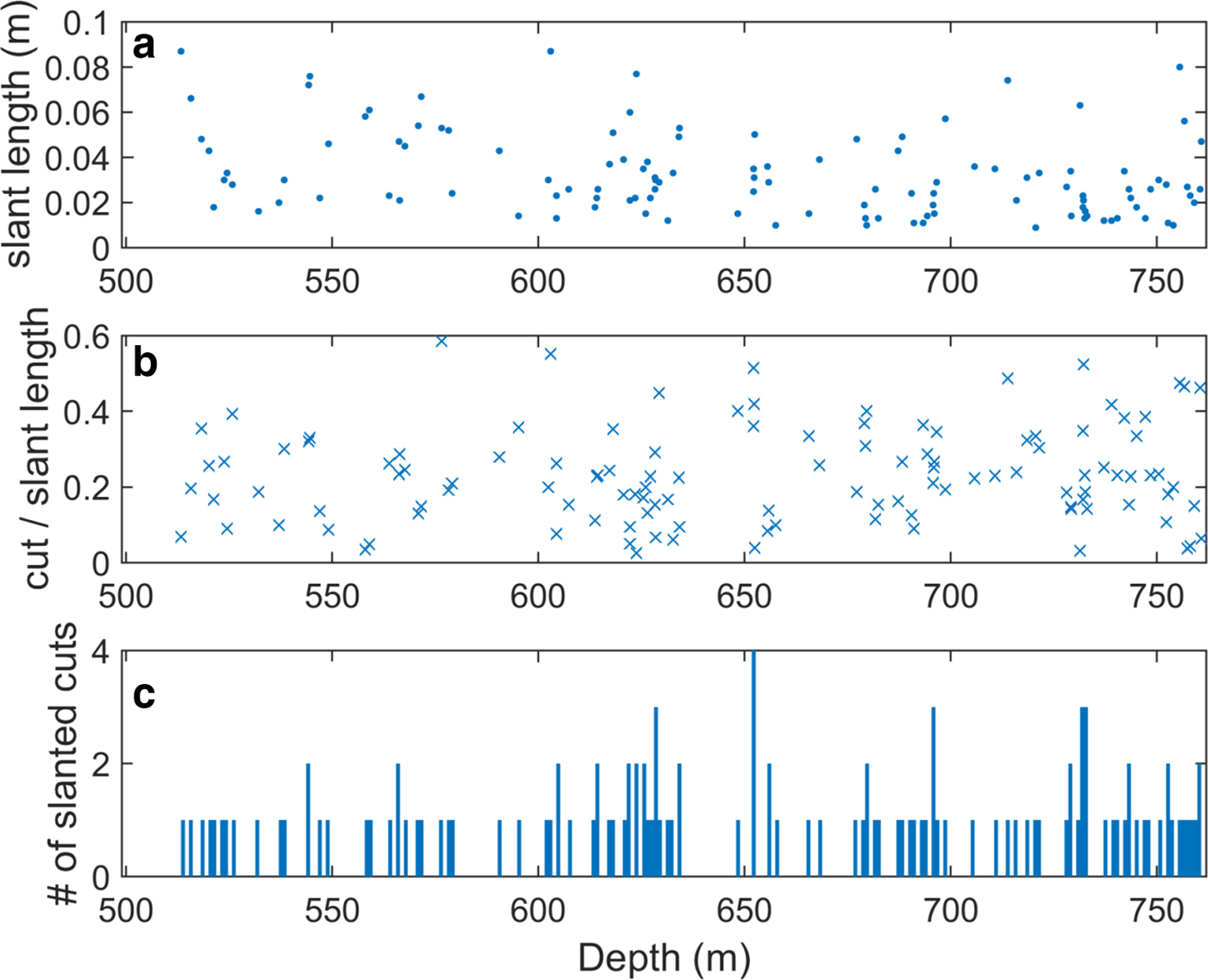
Fig. 5. The length and distribution of slanted breaks only. Top (a) plots the total length of each slanted segment (including the length of the piece removed) at the depth that it occurs. Middle (b) shows the ratio of the length of the piece removed to the total length of the slanted segment, giving an indication of the degree of smoothing to be expected. Bottom (c) shows the number of slanted cuts per meter vs depth.
3.2. Data smoothing
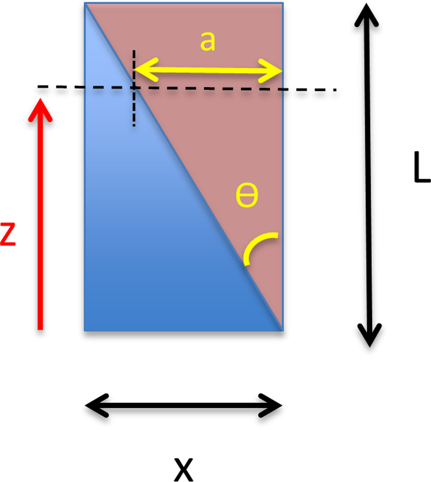
We first quantify the expected effect of a slanted break on the data. With perfect mixing between the two wedges of the slanted break, we expect an even smoothing. Each point in the data is mixed with another point a fixed distance apart (equal to the length of ice removed), using a linear weighting function:
 $$\delta = \; \displaystyle{a \over x} \times \delta _1 + \; \displaystyle{{x - a} \over x} \times \delta _2, $$
 $$\theta = \; \tan ^{ - 1} \displaystyle{x \over L},$$
 $$a = z\; \tan \theta, $$
where x = 34 mm (the width of the ice core), L = length of slanted segment, δ = mixed δ 2H or δ 18O, θ is the angle of the slanted cut, z is the relative vertical distance and a is the distance from the outer edge to the inner break edge (Fig. 6). This is the theoretical or idealized effect of introducing slanted breaks, which we compare to our data.
We are able to assess the actual effect of slanted breaks on the data, as there was one segment of core for which both the A and B sections were melted, and the B section featured a slanted break where the A section did not. This segment (core 498, spanning depths of 497–498 m and age of ~16 years ~5600 BP) is shown in Figure 7. The slanted break occurred between 497.54 and 497.64 m from which 1.4 cm in length was removed. The two sections were melted in different melting campaigns, with A melted in 2013 and B melted in 2014. It is unusual to have duplicate measurements that are both of high quality, as a second measurement was only carried out in the event of equipment or software failure during the first measurement. Section B of core 498 was measured as part of an initial equipment test and training run for the 2014 melting campaign, in which the CFA system and instruments ran without fault. The measurement of section A in 2013 was of excellent quality, with an acceptable amount of measurement error (Fig. 7), and was selected for inclusion in the final CFA dataset.

Fig. 7. The 15 s moving averages of δ 2H (a) and δ 18O (b) from core 498 A, melted in 2013, and 498 B, melted in 2014. The 2014 B data contain a slanted segment highlighted in orange. Also shown in cyan is a simulated slanted segment constructed with the data from 2013 A. To simulate the slanted segment, the continuous (unbroken) data from the 2013 A core have been smoothed according to Eqns (2–4) at the same depths where the actual slanted segment occurs in the 2014 B core. The uncertainty range of the 2013 A is drawn in black-dashed lines in both panels according to the point-by-point error calculated in Keller and others (Reference Keller2018). The average uncertainty over the length of the 498 A core is δ 2H = ± 0.85‰ and δ 18O = ± 0.23‰. The uncertainty range of the 2014 B data is drawn in red-dashed lines and is assumed to be the average error for the whole dataset, δ 2H = ± 0.74‰ and δ 18O = ± 0.21‰. For comparison, discrete measurements from the outer meltwater of the 2014 B core are shown with red stars. Error for the discrete measurements is δ 2H = ± 1.5‰ and δ 18O = ± 0.2‰.
The δ 2H and δ 18O data for both the A and B sections are overlaid in Figure 7, revealing some differences in the data over the length of the slanted segment. Also shown is the error range, which is the point-by-point error calculated for the 2013 A data (see (Keller and others, Reference Keller2018) for our error calculation methodology). The B data do not have the same rigorous error estimates because the measurements were part of an initial test run in 2014 and are not included in the final CFA dataset; we assume the overall average uncertainty of δ 2H = ± 0.74‰ and δ 18O = ± 0.21‰ for these data (Keller and others, Reference Keller2018). As expected, the data from B are smoothed relative to A; however, the key features (the large amplitude changes) are preserved and are still visible. Interestingly, the δ 2H data show a much larger difference than δ 18O, and the values are outside the uncertainty range, even after accounting for uncertainty in the B data. However, most of the δ 18O data fall within uncertainties. The average uncertainty over the length of the 498 A core is slightly higher than the overall average, at δ 2H = ± 0.85‰ and δ 18O = ± 0.23‰. We show the precise difference between the A and B data over the slanted segment in Supplementary Figure S10a. The difference between the A and B δ 2H data peaks at 3.9‰ at a depth of 497.584 m, much larger than the combined error of both measurements. In contrast, the maximum difference in the δ 18O data is 0.31‰ at a depth of 497.608 m, which is within the ±0.31‰ combined uncertainty. We note that the agreement between A and B sections is very good for the other parts of the core, and the difference is mostly within the given uncertainty.
To test our data against the expected mixing calculated from Eqns (2–4), we constructed a theoretical slanted break with the continuous, unbroken data from the 498 A core using the actual depth and length of the slanted break in the B core. Each point in the data is mixed with a point 1.4 cm apart. This simulated slanted break is drawn along with the actual data from A and B in Figure 7. The difference between the simulated break and the B section is shown in Supplementary Figure S10b. There is more smoothing introduced in the real slanted segment, particularly in the δ 2H data, and the amplitude changes are reduced. The maximum absolute difference between the simulated and real slanted segment in the δ 2H data is 3.7‰. The δ 18O data is much closer, with a maximum difference of 0.25‰.
Compared with our theoretical reconstruction, there is a more pronounced difference between the A and B δ 2H data over the slanted segment. The reasons for this discrepancy are unclear. In the actual melting process, there will inevitably be differences in the conditions from one melting period to the next. Our error estimates are designed to account for uncertainty in the calibrations, instrumental drift and noise (Keller and others, Reference Keller2018); however, it is evident that there are additional sources of error. Sections 498 A and B were melted in different years, and the setups in 2013 and 2014 differed (Emanuelsson and others, Reference Emanuelsson, Baisden, Bertler, Keller and Gkinis2015), which could affect the degree of smoothing. As mentioned previously, the B section was among the first cores melted in the 2014 campaign and was used as a training run, so there is potentially some added error in the operation of the instruments or CFA system. There is considerably more scatter in the raw data from section B (not shown), which could imply sub-standard instrument performance. There also could have been some vertical slippage of the core at the slanted break during melting. This was observed occasionally during the 2014 melting campaign and would cause a small misalignment of the two pieces across the break, in which case the location of the points that were mixed would not match the theoretical case.
Taken together, this implies that we have underestimated the uncertainty in the data over slanted breaks. To be very conservative, an additional error of ±3.0‰ (δ 2H) and ±0.10‰ (δ 18O) could be added to the data over slanted breaks, which would cover most of the discrepancy in the data presented here. For most analyses, some smoothing of the data and increased uncertainty would be preferable to large gaps with completely missing data. For comparison, the discrete measurements shown in Figure 7 have a resolution of ~2.0 cm; if we only had discrete measurements over the slanted break, it would be difficult to confidently identify the shape of the curve.
To explore the effect of slanted breaks further, we constructed a series of simulated slanted breaks with data from core 701 (spanning depths 700–701 m), chosen because this was a high-quality section with no actual physical breaks and was continuously melted in its entirety. The mean error for this core is δ 2H = ± 0.35‰ and δ 18O = ± 0.15‰. We simulate a slanted segment with 2.0 cm removed from a total length of 10 cm at different parts of the core (Fig. 8) so that the effect on different features in the record can be displayed. This is somewhat longer than the typical break, but we use this in our example so that the difference is visually noticeable. At this depth, 10 cm equates to ~22 years on our preliminary age scale (Lee and others in prep). The actual data are shown along with the simulated segments in Figures 8a–c.
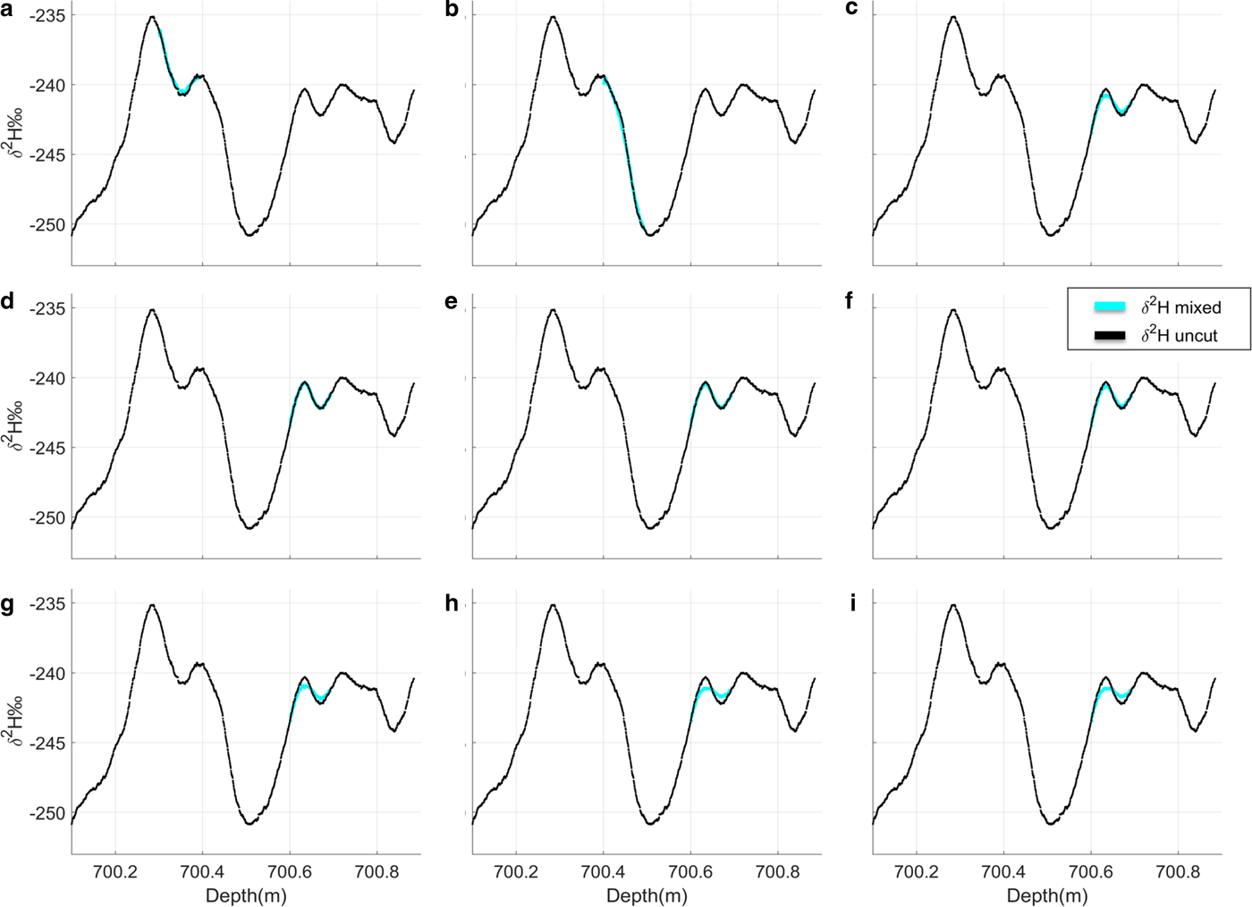
Fig. 8. Simulated slanted segments constructed with δ 2H data from unbroken pieces of ice. In (a–c), the amount removed is constant at 2 cm, and location within the core is varied: (a) 700.3–700.4 m; (b) 700.4–700.5 m; (c) 700.6–700.7 m. In (d–i), the location is the same (700.6–700.7 m), but the length of the piece removed is varied: (d) 0.5 cm; (e) 1.0 cm; (f) 1.5 cm; (g) 2.5 cm; (h) 3.0 cm; (i) 4.0 cm.
The slanted break has almost no effect on a steeply sloping curve, where the change in δ 2H is all in one direction (Fig. 8b); however, in sections where the isotopic value is changing direction rapidly and features include small peaks or dips, the smoothing effect is much more apparent (Fig. 8c). Similar to the actual example from core 498, the amplitude of the curve is smaller, but the fundamental characteristics of the signal are maintained, i.e. there is still a curve in the same position as the unbroken data.
We also simulate the effect of different cut lengths (the length of the piece removed) in Figures 8d–i, keeping the location of the break within the core (700.6–700.7 m) and the total length of the segment (10 cm) constant, but varying the amount removed between 0.5 and 4.0 cm. The smoothing is barely noticeable with a cut of 1.0 cm, but becomes more pronounced by 2.0 cm. A cut of 3.0 cm has a significant effect such that the small-scale features of the data would be difficult to interpret, with the change in amplitude becoming close to the uncertainty range. The shape of the curve is lost entirely when the cut is 4.0 cm (Fig. 8i), or 0.4 of the total length. We note that the data from core 498 showed more smoothing than would be expected from our model, implying that the loss of small features could occur with a shorter cut than suggested here.
The mean length of the slanted pieces (without ice removed) over the entire 261 m of core is 3.2 cm (median 2.7 cm), making most segments much smaller than the examples given here. The mean ratio of the length of the piece removed to the total length of the slanted segment is 0.23, so the degree of smoothing is similar to the 2.0 and 2.5 cm cuts shown in Figures 8c, g. The largest ratio of piece removed to total length is 0.61, and there are 15 cases where the ratio is >0.4 (see Fig. 5). These data should be analyzed with care; depending on the shape of the data at these locations, some features might be lost.
Melting slanted segments introduced an increase in uncertainty in the depth alignment of the CFA data. Because the edges of slanted breaks at times caught on the side of the holder, the core was temporarily stuck and the encoder reading was interrupted (characterized by a series of flat, constant readings followed by a sudden jump as the piece slid down). Although not unique to slanted segments, encoder slips tended to happen more frequently when the core contained slanted breaks. In our processing algorithm, we assumed a constant melt rate, and we linearly interpolated the depth over any time periods where the edges caught or the encoder did not work properly. However, this introduces a small error in the assigned depth, up to ~1 cm. From a qualitative inspection, there were more slips that required interpolation where there was a slanted segment. While these data required more processing time, the final, processed CFA stable isotope data over slanted segments was indistinguishable from the rest of the dataset.
As an unintended benefit, slanted breaks were more effective at expelling laboratory air and preventing potential contamination to the CFA methane data. As the ice core melts, a layer of water forms on the melt head before being drawn away by capillary forcing. This water layer did not grow but maintained a height of ~1–2 mm. Straight breaks at times captured a small bubble of laboratory air that was pulled into the inner melt line, mixing with the trapped air bubbles in the ice. However, slanted breaks provided an avenue for laboratory air to escape without being drawn down. While an analysis of the methane data is beyond the scope of this paper, this effect deserves more investigation in future studies.
4. CONCLUSIONS
Brittle ice is a challenge for all intermediate-depth and deep ice core drilling campaigns. Steps to take in the field to protect the integrity of the core before transport include using a hydraulic-powered system to provide the core break force during drilling and an active cooling refrigeration system to store the cores in the field. Once brittle ice is encountered during core processing, relaxing the ice at a warmer temperature for several months is important to minimize fractures from occurring in the first place. However, with careful processing and minor modifications to existing CFA system designs, many fractured pieces in the BIZ can be included in CFA measurements.
The technique we have developed to melt slanted pieces of ice allowed for a significant amount of valuable material to be included in CFA water isotope measurements. This was especially important as we reached the lower depths of the core, where the age-depth scale is compressed and each length of ice represents an increasing amount of years. We were able to include 3 m of ice (1% of the 261 m of brittle ice and ~1300 years of climate history) that otherwise would not have been available for CFA. There is some reduced resolution or smoothing in the data that resulted from mixing ice from different depths on either side of a slanted break, but major features of the stable water isotope data are still visible. The largest impact of slanted breaks occurs over data that include small, rapid amplitude changes, where (depending on the length of the break and the amount of ice removed) smoothing could obscure the features altogether. As we saw with the example of core 498, the degree of smoothing in the actual measurements could exceed that predicted from our model. We have likely underestimated the uncertainty in our dataset over slanted breaks. In cases with a large (>0.4) cut-to-total-length ratio, data should be interpreted with care. Nevertheless, a smoothed signal is preferable in most cases to data gaps and/or lower resolution discrete measurements.
We have so far only analyzed the effects of slanted breaks on the water stable isotope data. Examining other RICE CFA data (e.g. methane, calcium, dust, pH and conductivity) is beyond the scope of this paper but would be a useful topic for further study. While we expect the effects of smoothing to be well represented in our high-resolution stable isotope dataset, an analysis of other datasets with similar or lower resolution would serve as an important verification of our method.
SUPPLEMENTARY MATERIAL
The supplementary material for this article can be found at https://doi.org/10.1017/jog.2018.19
ACKNOWLEDGEMENTS
We are indebted to the 2013 and 2014 RICE core processing teams. We are grateful for the technical support of the GNS Science mechanical and electronic workshops and the GNS Science Stable Isotope Laboratory. We thank Jocelyn Turnbull for assistance in setting up the RICE data base. We also thank GNS Maori Relationships and Opportunities Advisors Diane Bradshaw and Bevan Hunter for their recommendation on naming the drill used to collect the RICE ice core. We thank all the people involved in the RICE logistics, fieldwork, sampling and analytical programs. We also thank the reviewers for their constructive comments that have improved this manuscript.
AUTHOR CONTRIBUTIONS
R. L. Pyne and N. A. N Bertler designed the method for melting brittle ice and led the melting campaigns in 2013 and 2014. E. D. Keller and S. Canessa analyzed and processed the CFA water isotope data. A. R. Pyne and D. Mandeno developed the drilling techniques and storage methods. P. Vallelonga and H. A. Kjær led the design of the CFA setup. S. Semper and E. Hutchinson developed the code in LabView to process the melt data. W. T. Baisden contributed to project design and data analysis. All authors contributed to the writing of the manuscript and have given approval to the final version of the manuscript.
FUNDING SOURCES
This work is a contribution to the Roosevelt Island Climate Evolution (RICE) Program, funded by national contributions from New Zealand, Australia, Denmark, Germany, Italy, the People's Republic of China, Sweden, UK and USA. The main logistics support was provided by Antarctica New Zealand (K049) and the US Antarctic Program. Funding for this project was provided by the New Zealand Ministry of Business, Innovation, and Employment Grants through Victoria University of Wellington (RDF-VUW-1103, 15-VUW-131) and GNS Science (540GCT32, 540GCT12), and Antarctica New Zealand (K049). The Danish contribution to RICE was funded by the Carlsberg Foundation's North-South Climate Connections project grant. The research also received funding from the European Research Council under the European Community's Seventh Framework Programme (FP7/2007–2013) ERC grant agreement 610055 as part of the Ice2Ice project.


 Open access