1. Generalities and Assumptions

In this paper the motion of flowing avalanches is calculated using some methods of technical hydraulics. Avalanching snow behaves differently from water, hence, the equations describing the flow model have to be adapted to the properties of snow. In doing so one has to consider the restrictions made by Reference SalmSalm (1968):

• (1) The material is ideal elasto-plastic, similar to a dry sand.

• (2) The flow is bi-dirnensional and steady, but non-uniform. This non-uniformity is caused by a change in the slope angle.

Furthermore, we assume the friction forces T along the avalanche track to depend upon velocity v like T = a₀v°+a₂v², where the a_i are constants. The viscosity term a₁v¹, is neglected (Reference SalmSalm, 1966). These limitations allow us to describe a flowing avalanche by the Bernoulli equation of non-viscous discharge.

2. Basic Equations

2.1. Velocity distribution in a curved channel

In a curved channel the velocity is not constant over the flow depth t, but changes with increasing z (Fig. 1), as shown by Reference FrankeFranke (1971):

(1)

R₀ is the constant radius of curvature at the flow surface and v₀ the surface velocity. The positive and negative signs are set for decreasing and increasing slope angles respectively. Equation (1) is only valid with a positive denominator. v₀ may be obtained from the continuity equation

where Q means the constant flow rate and B the flow width. Hence it follows that

(2)

and the velocity vt at the depth z = t

(3)

when R = R₀±t.

Fig. 1. Velocity distribution in curved channels.

2.2. Friction forces on the surface of the avalanche track

As suggested by Reference SalmSalm (1968), the shearing stress τ_xz between the avalanching snow and the stationary underground is considered to depend linearly upon the normal stress σ_z acting on the sliding plane, and also upon the square velocity v², the roughness of the avalanche track k^-2, and the mean gravity of the moved snow y, in accordance with the equation of Chézy for turbulent flow. Thus we assume

(4)

where μ is a dry-friction coefficient.

If the avalanche track is bent with an actual radius of curvature R, σ_z is set to

(5)

where ψ is the slope angle and g is the acceleration due to gravity.

Equations (4) and (5) do not depend upon the material, the only material term being y, thus these equations are valid for plastic and elastic materials.

By inserting Equation (3) into Equation (5) we get

(6)

The importance of the second term within the brackets grows with decreasing radius of curvature R.

2.3. Avalanching snow

In soil mechanics, soil yielding is often described by the Coulomb criterion for cohesive materials

(7)

where τ_xz is the shear stress and σ_z the normal stress on a plane element. τ_f stands for the shear strength, ø for the angle of internal friction and c for the cohesion of the considered material. As shown by Terzaghi (Reference Terzaghi and JelinekTerzaghi and Jelinek, 1954), Equation (7) leads to

(8)

in the case of plain strain. The directions of the stress symbols σ and ⊤ are explained in Figure 2 .

Fig. 2. Mohr-Coulomb hypothesis.

Equation 8 is perfectly compatible with general plasticity theory, as demonstrated by Reference Drucker and PragerDrucker and Prager (1951).

A dry sand is not cohesive (c = o), and in this case Equation (8) becomes

(9)

In an elastic material σ_x is given by the confined three-dimensional stress state (Reference ZieglerZiegler, 1962),

(10)

here v is Poisson’s ratio. Equation (9) is restricted to non-curved tracks.

As long as the stresses σ_z, σ_x, τ_xz, calculated from Equations (5), (10) and (4), do not fulfil the yield criterion (Equation (9)), the material remains elastic, but as soon as the left side of Equation (9) equals the right-hand side, Equation (10) is invalidated and σ_x is obtained from Equation (9):

(11)

where

The positive sign gives the maximum value σ_x1, corresponding to the passive stress state of Rankine, and the negative sign the minimum value σ_x2 corresponding to Rankine’s active stress state (Fig. 2).

3. Bernoulli’s Equation

Flow depths of non-uniform steady flow are generally calculated stepwise using Bernoulli’s equation

(12)

H denotes the energy head, p the pressure in flow direction x on the sliding plane, and w the geometrical head.

A friction force T per unit volume, divided by y, is obtained from Equation (4):

(13)

T/y corresponds to the gradient of the total head, and may be written as

from which we obtain

(14)

Δw_e is the energy loss per length Δu.

When the pressure p at the slip plane is replaced by σ_x cos ψ (Reference SalmSalm, 1968), the equation of non-uniform steady flow of avalanching snow becomes,

(15)

using Equations (11) (plastic case) and (10) (elastic case). Here the index u refers to an upper and the index l to a lower cross-section of the avalanche track (Fig. 3).

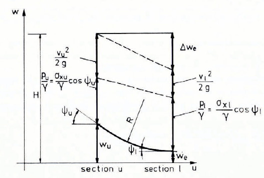
Fig. 3. Bernoulli’s equation modified for avalanches.

Plotting the specific energy H _e against flow depth t (Fig. 4), where

(16)

and F is a cross-section of the avalanche track, we obtain a minimum H_e for a critical value t _er. If, in a given flow, t ˃ t _er, this flow is called “streaming”, if t ˂ t _cr, it is “shooting”. A streaming flow changes continuously to a shooting one, this happens inversely in a “hydraulic jump”. Hydraulic jumps are calculated with the momentum theorem; in the continuous changes Equation (15) may be used as follows.

Fig. 4. Specific energy versus flow depth.

• 1. Calculate H at the first (known) point (Equation (15)).

• 2. Take next point: use geometry and an assumed value for t.

• 3. Calculate σ_z, σ_x (elastic), and τ_xz (Equations (6), (10), and (4)).

• 4. Is the yielding function (Equation (9)) fulfilled?

  • If yes then continue.

  • If no then go to step 6.

• 5. Calculate σ_x (Equation (11)).

• 6. Calculate Δ_e (Equation (14)).

• 7. Calculate H at the second point (Equation (15)).

• 8. Is Equation (15) fulfilled?

  • If yes then take the next point.

  • If no then go to step 2.

4. Experiments with the Test Slide

The same tests as those described by Reference SalmSalm (1968) were made, but with a modified snow collector which could contain 25 m³ of snow. A steady flow was maintained for more than 0.7 s with this modification. Every experiment was filmed, this allowed a measurement of the flow depths behind the deflection point.

Table I compares some test data from the slide inclined at 45° with the results of a step-by-step calculation using Equation (15). Two points o and 2 were calculated as shown in Figure 5, starting at the end of the acceleration part of the test slide and using measured values of velocity and flow depth. The calculations were made with friction coefficients μ and k as parameters, other values were ϕ = 26° and v = 0.25. The calculated flow depths at point 2 are those which give the best fit with the measured values. The corresponding friction coefficients are also shown.

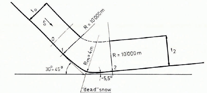
Fig. 5. Flow on test slide at Weissfluhjoch.

TABLE I. MEASURED AND CALCULATED FLOW DEPTHS FOR T _U = 1.0 m

We can divide these experiments up into two groups. The first 4 tests in Table I were made at low snow and air temperatures, without snow melting. The slide is dry and the friction is high. The remaining tests were carried out at temperatures near 0°C. The high temperature means that a thin layer of melted snow covers the test slide; this reduces friction. The values of μ_* were calculated using the known velocity v₀, for the acceleration part of the slide (without turbulent friction k ^-2).

Plots of H_e (Equation (16)), show a critical flow depth t_er > 1.5 m. All tests began with t₀ = 1.0 m, Table I shows that in all cases t₂< 1.20 m. Thus, we conclude that in these tests a continuous flow-depth change in shooting flow occurred without hydraulic jumps; this is confirmed by the cine film.

5. "Skilehrerhalde" Avalanche in Parsenn Area

The validity of our conclusions was tested with an artificially released avalanche near our institute; this has been described by Reference FrutigerFrutiger (1975)· Geometrical data for these calculations were obtained by fitting a cubic parabola to the natural avalanche track (Fig. 6).

Fig. 6. Track section of “Skilehrerhalde” avalanche, so January 1974, Weissfluhjoch/Davos.

Friction parameters were set to μ = o. 18 and k² = 1 700 m/s². Q was calculated with the formula given by Salm (Reference SalmSalm, 1972).

A formula for the runout distance x_r can be derived from Equation (15).

The velocity head v_u²/2g and the pressure head σ_xu cos ψ_u/γ disappear within the distance x_r = w_u/sin ψ_m due to friction Δw_e. Thus we write

and

Inserting Equation (14) we get

(17)

The steady-state equation of Bernoulli is not exactly valid for this case because velocity v is time-dependent. For this reason we have to calculate with mean values.

The quantities labelled with index m denote such values in the runout process. Assuming that the square of velocity decreases linearly along runout x_r, as suggested by Reference VoellmyVoellmy (1955) and Salm (1966), we get

(18)

and

(19)

The value in Table II was calculated with this formula and agrees well with the measured value of 224 m.

TABLE II. OBSERVATIONS AND DERIVED DATA FROM THE ARTIFICIALLY-RELEASED AVALANCHE