


1. Introduction
Understanding the ability of water to infiltrate into cold firn is fundamental to partitioning the fate of surface melt in Greenland's lower accumulation zone. Particularly important is the proportion of the pore space in the firn which is available to be filled with meltwater (e.g. Harper and others, Reference Harper, Humphrey, Pfeffer, Brown and Fettweis2012). Although there has been extensive theoretical and observational investigation of air movement and permeability of dense firn (e.g. Albert and Shultz, Reference Albert and Shultz2002; Courville and others, Reference Courville, Hörhold, Hopkins and Albert2010; Gregory and others, Reference Gregory, Albert and Baker2014), there has been far less effort directed at water motion in dense firn.
Prior infiltration studies have focused on relatively shallow conditions (Braithwaite and others, Reference Braithwaite, Laternser and Pfeffer1994; Pfeffer and Humphrey, Reference Pfeffer and Humphrey1996; Harper and others, Reference Harper, Humphrey, Pfeffer, Brown and Fettweis2012; de la Peña and others, Reference de la Peña2015; Charalampidis and others, Reference Charalampidis2016), where relatively low firn density is commensurate with high pore space, and the framework is easily accessible to surface melt. However, a substantial fraction of the total pore space in the firn column exists below 10 m depth (Leone and others, Reference Leone, Harper, Meierbachtol and Humphrey2020). Infiltration has been observed to >10 m on the GrIS (Humphrey and others, Reference Humphrey, Harper and Pfeffer2012; Miller and others, Reference Miller2020) and the top of liquid-filled pore space (i.e. firn aquifer) may be tens of meters below the surface (Forster and others, Reference Forster2014; Miège and others, Reference Miège2016). The limits on infiltration depth are unclear: pore close-off is a definite barrier, but water flow should become progressively restricted as the framework becomes colder and denser, causing increased freezing and slow flow. Once an aquifer is in place, the temperature, density and grain structure of the firn at the lower boundary prior to formation is essentially unobservable because of alterations that have taken place (Koenig and others, Reference Koenig, Miège, Forster and Brucker2014). Thus, uncertainty about the thermal and density constraints on water flow leads to uncertainty about deep infiltration and future expansion of firn aquifers.
Most large-scale modeling of the fate of meltwater in firn, including the common bucket scheme, is based on a simple balancing of the amount of meltwater with the ability of the cold snow and firn to refreeze that water (e.g. Pfeffer and others, Reference Pfeffer, Meier and Illangasekare1991; Ligtenberg and others, Reference Ligtenberg, Helsen and van den Broeke2011). Essentially, this energy-balance approach concludes that melt will penetrate to the depth at which the vertically integrated cold content of the firn matches the amount of water to refreeze. Downward flow depends on a relationship between temperature of the firn (T firn), and firn density (ρ firn). A saturated water front stops if the cold content of the firn is greater than the latent heat of the saturating water:

where the left-hand side includes heat capacity (C p) and is thus, the cold content, and the right-hand side is the saturated water content (in brackets) and latent heat of fusion (L h). The density of ice and water used in this paper are 920 and 1000 kg m−3, respectively.
This simple energy balance places a rough limit of the depth of meltwater infiltration based simply on cold content. For typical firn densities and temperatures observed in the Greenland percolation zone (~−20°C), Eqn (1) predicts that all firn pore space is available for saturated meltwater infiltration. Details of water and heat flow must be considered in the context of the framework of the firn to advance beyond this simplified scheme. An end-member approach is to consider the firn as a continuum with appropriate parameterizations for the volume-averaged quantities (Meyer and Hewitt, Reference Meyer and Hewitt2017). The opposing end-member is a grain-scale approach, focusing on the geometry of the matrix and pore structure, which is often implemented in the hydrocarbon reservoir modeling field (e.g. Sun and others, Reference Sun, Tang, Espinoza, Balhoff and Killough2018), but to our knowledge has not been applied to firn.
Here, we investigate deep penetration of meltwater into cold and dense firn. We employ both observational and modeling methods to constrain the firn structure, density and temperature conditions that permit or inhibit migration of a saturated water front. We first present in situ experiments conducted in Greenland's percolation zone, where water was pumped through the full thickness of the firn column with sensors in place to monitor water and heat flow. Field observational data are then used to develop a simplified grain-scale firn model for heat and water transport. Our observational and modeling results reveal the physical limits on the migration of water in polar firn.
2. Field methods
2.1. Greenland field sites
Our field experiments were conducted at two sites along the Expéditions Glaciologiques Internationales au Groenland (EGIG) line of Western Greenland (Fig. 1). Both sites are well within the percolation zone, experiencing numerous summer melt events and ice layer development, but are well above the soaked and runoff zones, and regions of natural firn aquifers (Humphrey and others, Reference Humphrey, Harper and Pfeffer2012). Site CP is at 2000 m and is located 1 km from the Crawford Point weather station (Steffen and others, Reference Steffen, Box and Abdalati1996); site T3 is ~30 km down-glacier at ~1800 m elevation. This section of the EGIG line has been the focus of numerous investigations focusing on firn processes, which have taken place over a period of several decades (e.g. Benson, Reference Benson1962; Braithwaite and others, Reference Braithwaite, Laternser and Pfeffer1994; Harper and others, Reference Harper, Humphrey, Pfeffer, Brown and Fettweis2012; Humphrey and others, Reference Humphrey, Harper and Pfeffer2012). Relevant legacy data from these studies include stratigraphy, temperature and density profiles from the upper 10 m (Harper and others, Reference Harper, Humphrey, Pfeffer, Brown and Fettweis2012; Humphrey and others, Reference Humphrey, Harper and Pfeffer2012), and characterization of firn density to 100 m depth (Brown and others, Reference Brown2012; Higgins, Reference Higgins2012).

Fig. 1. Western Greenland site (a) and regional (b) setting. Gray lines in (a) show surface elevation contours at 200 m intervals.
2.2. Borehole drilling
At each of the two field sites, multiple boreholes were drilled to 65–100 m depth, penetrating all or nearly all of the firn column. Three boreholes were drilled at site CP, one to 100 m depth and two to 65 m depth. Two holes were drilled at site T3, one to 100 m and one to 65 m. In addition, at least one core to 30 m depth was extracted at each site using a standard core drill and logged for density and stratigraphy.
Deep boreholes were drilled with a custom hot-water drill system designed for drilling in firn (Humphrey and others, Reference Humphrey, Harper and Meierbachtol2020). Our drill system advances a borehole through the firn by melting a ~0.15 m diameter hole with a jet of hot water. The drill water was set at a moderate temperature of 50°C, and we drilled at a constant rate of 1 m min−1, thereby pumping 30 L min−1 through the outlet nozzle as the drill stem advanced through the firn package.
2.3. Borehole instrumentation
Immediately after drilling, the boreholes were logged with a recording video camera. The camera accurately locates the water surface in the boreholes and reveals characteristics of the borehole walls and the locations of major ice lens. After video logging, all the boreholes were instrumented with digital temperature sensors at 1 m spacing. The temperature sensors at site T3 have an accuracy of 0.1°C and a resolution of 0.0078°C, whereas the sensors at site CP have an accuracy of 0.25°C but a resolution of 0.0039°C. The laboratory-calibrated sensors are potted in epoxy for water proofing and durability. In the electrically and thermally isolated firn environment, the sensors show almost no noise at their max resolution. The boreholes were not back-filled, but were sealed at the surface, thus sensors above the water level may have been sampling the borehole air, not directly the firn. Data were logged for >1 year at either 15 or 30 min intervals.
2.4. Water penetration and thermal recovery experiments
Our methodology for hot water drilling deep boreholes presented a novel opportunity to monitor the fate of liquid water introduced to the firn package as the drill hole advanced. The borehole drill included an instrumented drill stem that records borehole water pressure and water temperature 2 m above the actual drill tip (Humphrey and others, Reference Humphrey, Harper and Meierbachtol2020). The drilling data allow for reconstruction of the height of water (if any) in the borehole during drilling and recording the temperature of the return water (if any) coming back up the borehole. When infiltration exceeded the rate of drill advancement the hole remained air-filled. Temperatures recorded in the air-filled portion of the borehole are dominated by the leakage of heat from the internal flow of hot drilling water and do not accurately represent the borehole air temperature. The long-term fate of the ~3 m3 of water pumped into the firn package during drilling was tracked from its thermal signature recorded by borehole instrumentation.
Drilling creates a thermal disturbance, bringing the entire firn column to 0°C in the immediate vicinity of the borehole. Subsequent decay of this thermal disturbance records the radial flow of heat away from the hole region into the surrounding cold firn. Drilling creates three major heat reservoirs: (1) the firn around the entire hole is warmed toward 0°C during drilling; (2) any water infiltrated into the firn adds the energy of latent heat of freezing, as well as adding density and thus heat capacity and, (3) the water-filled section of the borehole also adds latent heat of freezing. The decay time of this thermal disturbance is proportional to the magnitude of the heat disturbance reservoir.
3. In situ results
3.1. Initial firn conditions
At both T3 and CP, depth–density profiles show a general trend of increasing density with depth, broken by numerous swings to high density due to centimeter-thick ice layers (Fig. 2). Firn temperatures at both sites are cold. Temperatures at 30 m depth are −18 and −14°C at CP and T3, respectively. At 60 m depth, temperatures at the sites fall to −19 and −16°C. Densities at 30 m depth are ~660 and 700 kg m−3 at CP and T3, respectively. The trend in the T3 density profile can be reasonably approximated by steady firn densification in the presence of melt (Reeh and others, Reference Reeh, Fisher, Koerner and Clausen2005). At site CP, comparison of our detailed density data collected in 2018 with data collected in 2007 (Brown and others, Reference Brown2012; Higgins, Reference Higgins2012) indicates a negligible change in density during the past 10 years. Based on these data, the depth of pore close-off density (830 kg m−3) is ~75 m.

Fig. 2. Density profiles at sites CP (a) and T3 (b). Measured densities in 2018/19 are shown in black. Modeled temperatures based on measured temperatures are shown in red. Blue dots in (a) indicate 2007 densities (Higgins, Reference Higgins2012).
3.2. Water penetration
Records from the instrumented drill stem reveal real-time interactions between drilling water and the surrounding firn as the drill stem advanced through the firn column. The drill stem pressure and water temperature records from drill holes at sites CP and T3 have consistent characteristics (Fig. 3). From the surface to near 40 m depth, the erratic and warm drill stem temperature shows the borehole remained air-filled as the drill advanced, meaning that the drilling water soaked into the firn faster than the drill advanced. Erratic temperatures are created when the warm drill stem occasionally touches the rough firn walls of the hole, something only observed in air-filled holes because of the rapid thermal equilibration in a water-filled hole.
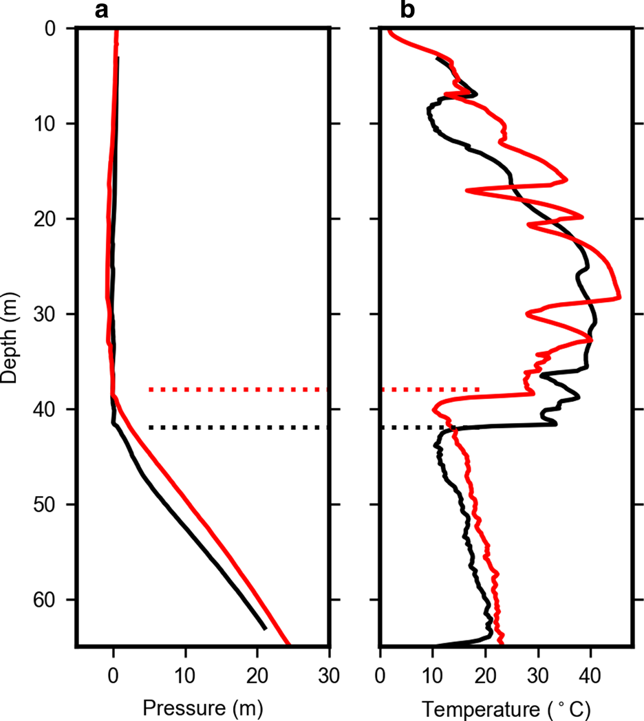
Fig. 3. Borehole water pressure (a) and temperature (b) measured by the instrumented drill stem during drilling CP (black) and T3 (red). Pooled water was encountered at depths of 38 and 42 m at sites CP and T3, respectively (dotted lines). Depths are approximate since they are derived from drilling speed records.
The drill stem pressure records reveal the rapid development of a borehole water level as the drill advanced through the firn column. At site CP, the water level appeared at 42 m depth, and at T3 the water level was a slightly shallower at 38 m depth. As the drill stem advanced into a water-filled borehole, the pressure follows the expected hydrostatic increase for a water-filled hole with a fixed water surface, indicating that the inflow rate from the drill was sufficient to keep the borehole water level approximately constant as drilling continued.
At the depths corresponding to the borehole water level, the drill stem temperature records abruptly cool by >10°C and stabilize in the water-filled borehole. Once submerged, the drill stem measures the temperature of water returning up the borehole from the drill tip. Although the thermal decay length of return water is longer than the 2 m between the drill tip and sensor (Humphrey and Echelmeyer, Reference Humphrey and Echelmeyer1990), the up-flowing water loses much of its heat close to the drill tip. The monotonic increase in temperature below the water level represents a slow progression toward a steady state drilling temperature in a water-filled borehole with no leakage. Lack of leakage from the hole into the surrounding firn was confirmed by repeat video logging ~1 h after drilling completion, which found a steady water level in the borehole.
3.3. Thermal recovery
Three distinct regions of the firn column are observed in the thermal decay records at each site (Fig. 4). Firn temperatures in the lowest region (below ~45 m depth) decay most rapidly. Initial temperatures in this region are above the freezing point due to warm drilling water, but temperatures fell to 0°C rapidly and the water-filled hole completely froze closed in only a few hours. Within 8 d, the lower thermal profiles were <1°C warmer than the ambient firn. The upper section of the boreholes (above the observed water-table) shows a slower and more complex thermal decay. This upper section of the hole is air-filled, and the sensors may not be well coupled to the firn. After 8 d, temperatures remain >1°C above the local ambient temperature.

Fig. 4. Time evolution of the thermal decay in CP (a) and T3 (b) after drilling. Curves show temperatures immediately after drilling (d 0), and thermal decay over the subsequent 8 d. The final temperature profile is from 3 months after drilling and does not show the upper 10 m since this is season dependent. The last depths to remain unfrozen are indicated by the dotted black line. These occurred at 39 m at site T3 ~4 d after drilling, and 44 m at site CP ~6 d after drilling. The CP data shown are from a 100 m hole, which had ~1 m3 more water pumped into the aquifer than at T3, which shows a 65 m borehole.
A distinct third region of the decay profiles exists in a 3–5 m thick section between the upper and lower sections described above. Thermal recovery here is quite slow, with unfrozen conditions persisting for several days. By 8 d, the layer remains 3–5°C warmer than ambient.
4. Interpretation of results
4.1. Creation of a perched aquifer
At both sites, the much-delayed thermal recovery at depths between ~39 and 44 m indicates a larger heat source existed at this level than above or below. Liquid water is the only possible source. Indeed, radial saturation of firn pore space around the borehole can produce a heat source far exceeding the water stored in the borehole below. We therefore conclude that during drill penetration a layer of firn several meters thick was completely saturated with water. We refer to this saturated layer as a perched firn aquifer. The thermal recovery signals show an asymmetric top-down decay, suggesting the upper ~2 m of the aquifers drained (assumedly by lateral spreading, since there is no thermal signal of vertical seepage) during recovery, leaving the lower 2–3 m fully saturated layer to slowly refreeze by thermal conduction.
The aquifer at CP formed at 44 m depth, where the density is 725 kg m−3 and the ambient temperature is −18°C. From the drilling records, we estimate that a total of ~3 m3 of water was pumped into the aquifer. Assuming water flooded the available porosity, about half of the pore-water refroze before the firn mass warmed to 0°C. Therefore, there was ~50 kg m−3 of liquid water in the fully saturated firn of the aquifer. Assuming the aquifer formed a saturated disk around the borehole, then the water could be accommodated in the fully saturated firn with a thickness ~3 m and a radius of 3 m.
The data are similar at T3, where the perched aquifer formed at 39 m with estimated firn density of ~750 kg m−3 and a warmer temperature of −14°C. However, the T3 thermal decay record is more complex, indicating that a lower layer, probably of lower density, was partially saturated 2 m below the thicker layer. The lower layer refroze more quickly. Considering the extensive variability and density layering we measure, such complexity should be expected.
In both experiments the temporary firn aquifers were ‘perched’ because they sat on top of open pore space, having formed at firn densities ~100 kg m−3 less than the pore close-off density (Fig. 5). With an open supply of liquid water, the energy barrier at the base of the aquifers set by Eqn (1) could be overcome easily, and so it is unclear why vertical migration of water was halted. We next address this question by examining the details of grain-scale heat and water flow.

Fig. 5. Schematic diagram of drilling experiment, showing time progression of the (orange) drill hose from the surface drill rig, into deeper, denser firn, with pooling water at depth. Actual firn densities given in Figure 2.
5. Simulating water and heat flow in dense firn grains
Our objective is to investigate the temperature and density states of cold firn that create an impermeable barrier to a saturated wetting front and which would form the depth limit of a firn aquifer. We first construct an idealized model for evolving a firn grain lattice, which allows varying the density, including the pores and joining constrictions, in a mass-conserving scheme that broadly mimics the actual cold firn densification processes. We then conduct simulations of water and heat flow across the grain lattice model.
5.1. Grain geometry
Our firn grain lattice model occupies a 3-D uniform cubic lattice of cells. Each cell of the lattice encloses a single firn grain of unspecified size. At lowest density, the grains are assumed to be octahedra, in cubic close packing, with vertices touching (Fig. 6a). This 3-D arrangement is uniform, homogeneous and extensive. To make the modeled firn more dense, we shrink the lattice, and squeeze each enclosed firn grain in a manner which preserves grain volume (i.e. mass) in each cell. As the enclosing cell shrinks, the octahedra do not shrink, instead the points of the octahedra which would overlap into adjacent cells are truncated, and that volume is added uniformly to the faces of the truncated octahedra inside the cell (Fig. 6b). This shrunken lattice of truncated octahedra defines the grain shapes, as well as the shapes of the pore spaces between each set of eight octahedra, and the flow constrictions, formed by four framing octahedra, joining each pore space (Fig. 6c).
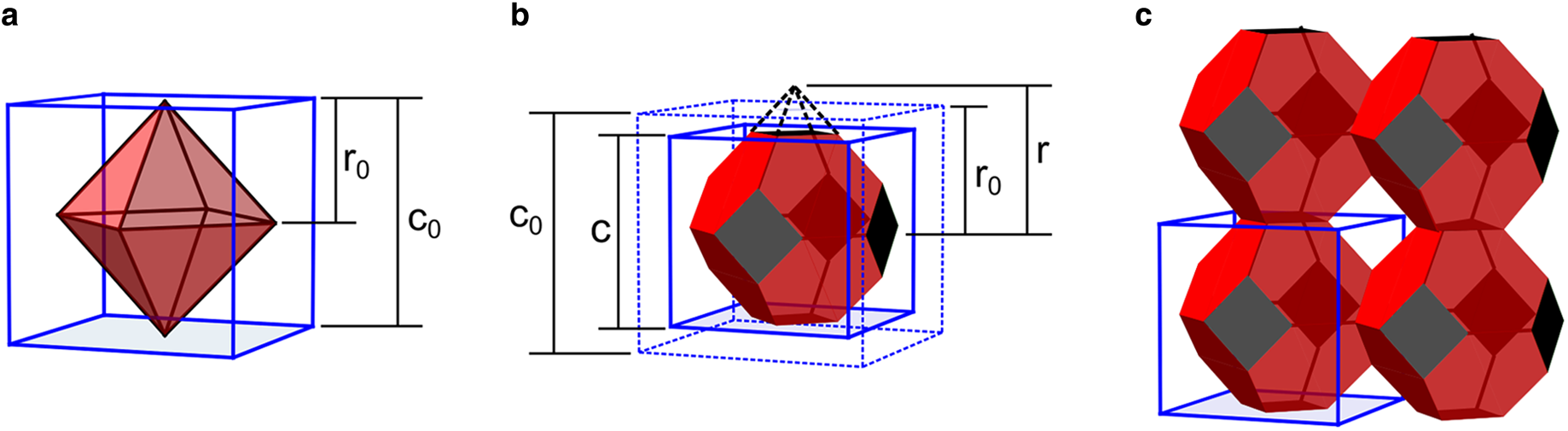
Fig. 6. Grain-scale model geometry. (a) Octahedron in the initial uncompressed and un-truncated state (red), enclosed by cubic cell lattice (blue). Cell size is the edge length c 0, whereas the octahedron size is the half diameter r 0. (b) Compressed cell and enclosed truncated octahedron. The enclosing cell is reduced in size from the initial c 0 (dotted blue) to c (solid blue), whereas the radius of the octahedron is enlarged (r 0 up to r) to allow the volume of the truncated octahedron to remain constant during compression. It is assumed that the truncated pyramidal mass (dashed black lines above the truncations) is transferred uniformly to the (red) octahedron faces. (c) Lattice of four octahedra showing stacking arrangement, connections and pores, in a compressed state. The model firn density of the illustrated arrangement is low (460 kg m−3) to make the packing and geometry easier to view. A compressed cell is outlined surrounding the lower left firn grain.
We force our firn model to match two characteristic density values: full density at an ice density of 920 kg m−3, and closure of pathways between pores at a close-off density of 830 kg m−3. To achieve these values in our lattice, we modify the octahedra faces to be slightly bulged (or cumulated) with low triangular pyramids. The bulges have a relief of 2.25% of the diameter of the octahedron and modify the octahedra into somewhat flattened triakis octahedra. Bulging the faces increases the density so that closing of the inter-pore flow constrictions occurs at a density of 827 kg m−3. For convenience, we continue to refer to these bulged particles below as octahedra.
5.1.1 Geometric length scaling
The firn grain lattice is completely specified by two length scales: the edge length of the bounding cubic lattice cell (c) and the one-half diameter of the octahedron particle (r) (Fig. 6). Note that r includes both the parts of the octahedron, that is inside the cell plus the height of the truncated part which does not exist (octahedra are normally scaled by their edge length, but this is less convenient in this study).
Using these fundamental measures, the volume of the bounding cell is c 3. The volume of a bulged octahedron is $V( r ) = 4/3r^3 + 4\;r^3f/\sqrt 3$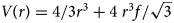 , where the first term is the volume of an untruncated octahedron, and the second term adds the volume of the eight bulged faces. The variable f is the ratio of the pyramid height to r, which we set to be constant at 0.045 in order to satisfy the constraint that the air close-off density is ~830 kg m−3.
In the fully compressed state, at a density of 920 kg m−3, both the cell and particle volume are c 3, where r reaches a maximum of 3c/2. The particle volume (V 0) stays constant for the particle, even though its shape changes as the enclosing cell size changes. This leads to the non-intuitive relationship that r is largest at full compression when most of the octahedron is truncated.
Particle volume (mass) conservation requires a relationship between c and r, as compression of the lattice changes, so that V(r, c) = V 0. An expression for the volume of a truncated bulged octahedron (V(r, c)), that has been truncated by the enclosing cell is algebraically complicated, but is given in Appendix A, along with several other useful geometric relations for bulged octahedra. This places a cubic polynomial relationship between r and c, which allows us to calculate or eliminate r for any cell size. There is a direct inverse relationship between the size of the cell and the model firn density.
The algebraic complexity of the polynomial relationship between r, c and therefore the density, requires numerical solution. However, there are three main derived dimensions from this constructed model: volume of the pores, size of the inter-pore constrictions that control water flow and the contact area of the grain-to-grain boundaries that control heat flow in the firn matrix. Length scales for these are given here in terms of r and c, which only apply to densities below air close-off.
The pore-to-pore water flow path is through a constriction with a square cross-section, and its size is scaled by edge length $L_{constrict} = \sqrt 2 ( {c-r} ).$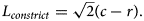 Pore shape is approximately a truncated octahedron with a length scale of $L_{pore}\cong \root 3 \of {( {c^3-V_0} ) }$
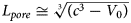 . The grain-to-grain contact area used for heat flow is approximately square, with edge length scale of $L_{contact} = {\rm \;}\sqrt {2( {1 + b} ) {\rm \;}} {\rm \;}( {r-c/2} ) , \;$
 where b is a correction for the bulges on the faces. The value of b is ~0.12, and is developed in Appendix A.
5.2. Water and heat flow
The firn lattice model is used as the domain for simulation of water and heat flow at the grain scale. Further simplifications avoid full 3-D modeling by assuming that water only flows in one of the cardinal directions of the cell lattice (the vertical direction). Cross-lattice connectivity is irrelevant since water is assumed to advance as a uniform front. These assumptions allow the water flow model to consider only one flow path made up of a series of pore spaces and constrictions, all in one straight line. Heat either flows perpendicular to water flow, directly to the surrounding grains, or from grain-to-grain in the water flow direction.
5.2.1 Water flow
In dense firn, the flow paths for water are sub-millimeter in size, and the gravity head gradient for vertical saturated flow is of order one. We start by assuming Poiseuille flow for the water and use length scales of the lattice model from the previous section. A scale for water flow velocity through a constriction is, v water = ρ waterg(L constrict/2)2/(8μ), where μ is the water viscosity, and ρ water and g are water density and gravity. We stress that this is a scale velocity, since the flow region is short and rectangular, and not a circular long pipe and the Poiseuille approach can give results that are too fast for short pipes. We do not use a continuum estimate based, for example, on the groundwater Kozeny–Carman relationship, which has been used in several previous discussions of water flow in snow (Gray, Reference Gray1996; Meyer and Hewitt, Reference Meyer and Hewitt2017). The Kozeny–Carman relationship breaks down at high firn densities, for example predicting finite water velocities past close-off density, all the way to full ice density.
To advance through both a constriction and a pore, the water front must fill each pore as it traverses past a grain. Assuming that the pore adds little drag to the flow, but does require filling, yields a scale for the water front velocity based on the time to fill the pore, $v_{front} = v_{water}cL_{constrict}^2 /L_{pore}^3$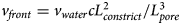 .
.
5.2.2 Heat flow considerations
An advancing water front is effectively a moving 0°C thermal front. The main flow of heat is perpendicular to the water flow direction and into the cold firn grains that constrain the water flow path. The thermal diffusivity of ice is of order 10−6 m2 s−1, and so the timescale for heat to flow from all sides into a millimeter-sized ice grain, for example, is somewhat <1 s. However, heat can also flow ahead of the water front through the grain-to-grain contact areas. If the water velocity is slow compared to the heat flow, the local grains are warmed while the water front has not flowed past, and significant heat can diffuse ahead of the front. Conversely, if the water velocity is fast compared to the rate of heat flow warming the local grains, little heat is lost to diffusion ahead of the water front. Note that in this fast flow case, the lack of complete grain warming does not affect the total freezing around a grain. Some water may escape into the next grains, but the eventual volume of local freezing will not be affected since slow water flow in high density firn contains no sensible heat and negligible flow energy.
Consideration of this lattice firn model indicates that freezing the pore-to-pore flow constrictions will stop water flow, leaving unfrozen water in the pore spaces. The volume of the pores would be reduced by freezing a rind of ice over the grain surface of thickness a little less than one-half the length scale of the constriction. Firn with this amount of refreezing would be impermeable, with free water in the pores, and the ice grain temperature would be the melting point.
We therefore modify Eqn (1) to consider only the sink of energy needed to freeze the pore-to-pore constrictions closed to water flow. At the same time, a similar layer will freeze over the walls of the pore:

The $3/\sqrt 2$ term on the right adjusts for the approximately octahedral shape of the pore, and the refrozen thickness (slightly less than L constrict/2) required to close the constriction.
An extra term, Q diff, is added to the left-hand side of Eqn (2) to account for heat lost to diffusion ahead of the water front, if important. There are two cases to consider. In the case of fast water flow past grains, determining the amount of freezing can be achieved with a local heat energy balance as given by Eqn (2) without the term Q diff. However, for slow water flow the additional heat lost to diffusion ahead of the front must also be considered to determine the amount of freezing. We investigate this non-trivial term, Q diff, in more detail below.
5.3. Heat diffusion ahead of a slow-moving water front
For a slow-moving water front, significant heat can diffuse ahead of the front, complicating the evaluation of Eqn (2). To obtain a scale for Q diff we consider a spatial reference frame moving with the water velocity, which we assume to be uniform. In this frame, the front is stationary and heat flows from the front into the firn, whereas the firn is effectively advecting toward the front. In this reference frame, the energy balance and temperature field are well described by solutions to the advection-diffusion equation. Figure 7 shows the appropriate transient advection-diffusion solution. Space is normalized by k firn/v front, where k firn is the thermal diffusivity of firn (Appendix B), and time by $k_{firn}v_{front}^{{-}2}$ .
.

Fig. 7. Non-dimensional plot of the transient advection-diffusion temperature ahead of a moving water front. Length is normalized ($k\;v_{front}^{{-}1}$ ), and temperature is normalized by initial firn temperature. In this moving reference frame (Lagrangian) plot, the x-axis translates to the right at the water front speed. Orange to black lines illustrate temperature evolution from initial (orange) to steady state (black). Steady state temperature is reached when the diffusion of heat from the water front is matched by the rate of advection of cold swept out by the advancing water front. Blue line is temperature at non-dimensional time of one.
Of particular interest in calculating the importance of Q diff is a scaling relationship that defines whether the water flow is significantly faster or slower than the heat flow. This is the Peclet-like dimensionless number scaled to the grain size (cv front/k firn), where c is the grain size. If this number is of order one or larger, then heat does not diffuse appreciably ahead of the front. A number <1 implies that the front is losing heat to grains ahead of the front, not merely to the local grain. Since k firn is approximately constant, this number mainly varies with cv front, and heat is only lost from the region of the local grains if the firn is very fine grained or the water front is very slow.
If the water front advances until a steady state is reached, where the front is advancing as fast as the diffusional heat ‘wave’ is advancing ahead of it, then the front reclaims any heat lost to warm the firn, and there is effectively no further heat lost from the front. However, during initial infiltration the warm front supplies heat to this warmed region ahead of the front, and during this transient time there is therefore an additional heat sink to freeze and halt the front advance. It is this transient heating that is the numerical value of Q diff. The length of time to reach a steady state is inversely related to the front velocity, and slower fronts lose more heat.
To give concrete examples, Figure 8 illustrates two specific cases of the heat flow ahead of slow and of fast water flow (Peclet number <1 and >1). The important timescale is the timescale for water to flow past a single grain, $c\;v_{front}^{{-}1}$ (dashed blue line in Fig. 8). The amount of heat that diffuses ahead of the front during that timescale is the value of Q diff, which is shown by the red area under the curve.

Fig. 8. Dimensional plots, based on Figure 7, illustrating diffusional heat loss under scenarios of a slow (a) and a fast-moving (b) water front. Firn grain size in both plots is 1 mm, represented by the dashed blue line. Peclet numbers in the slow- (a) and fast-moving (b) front scenarios are 0.2 and 2, respectively. Black lines reflect steady state temperature, and red lines reflect temperature profile at the timescale for the water front to flow past the first firn grain. Red shading illustrates heat lost during this time to diffusion ahead of the firn grain. In (a), heat loss ahead of the local firn grain is two times the heat lost to the grain. In (b), heat loss ahead of the water front is just 2% of heat loss to the local grain.
6. Simulation results
Our simulations provide constraints on conditions where the water in inter-pore connections freezes and reduces the firn to an impermeable state. To apply Eqn (2), it is necessary to determine the Peclet number, and thereby the importance of Q diff. If the Peclet number is large, Eqn (2) directly gives the density and temperature state that will make the firn impermeable. These high Peclet number states are shown by the blue line in Figure 9. These states require the firn to be less than half as cold as the simple energy balance of Eqn (1) to stop saturated water flow. Stated differently, refreezing of constrictions renders firn impermeable at densities that are ~60–100 kg m−3 less than close-off density under commonly measured firn temperatures (−10 to −20°C).

Fig. 9. Measured and modeled density and temperature conditions of pore close-off. Black line shows the prediction of Eqn (1), which is the temperature/density state required to completely freeze all the water in a saturated front. Blue curve shows the model prediction (Eqn 2) of water close-off, assuming the water front moves sufficiently quickly so that heat is not lost ahead of the front. Green curves show the predicted close-off conditions for heat loss ahead of slower water fronts created by high density and two grain sizes: 1 mm (dashed) and 2 mm (solid). Measured close-off conditions at CP and T3 are shown in red, with 20 kg m−3 density uncertainty bounds. Dashed gray line marks density of 830 kg m−3.
6.1. Grain-size effects
Our results show that when the constrictions are open enough to facilitate fast water flow and a high Peclet number, the close-off density/temperature in Eqn (2) is independent of grain size. This result may not be intuitive since the linear or areal size of the constriction is being frozen by the volumetric heat lost to the firn particle, which might imply a scale dependence. However, since the pore also freezes with a layer of similar thickness, freezing the constriction is a volumetric freezing to a volumetric heat sink, and is therefore scale independent.
The scale independence is upheld from a volumetric perspective at all grain sizes, but diffusional heat loss has the potential to substantially alter Eqn (2) under conditions of small grain size. We do not know the average grain size at the aquifer depths at our field sites, but we extrapolate from our 30 m cores to predict the sizes to lie in the range of 1–2 mm diameter. The water flow velocity for these sizes yield Peclet numbers near 1, and require further investigation. To illustrate the effect of grain size we use two different lattice sizes. We use lattices that will compress to grains of 1.0 or 2.0 mm3 cubes when the lattice is compressed to the full density of 920 kg m−3. The air pore close-off for these lattices occurs at density 827 kg m−3, and at lattice spacings of 1.037 and 2.07 mm, respectively. The lattice model is used to calculate the additional heat lost Q diff, and the strong effect of grain size is shown by the green curves in Figure 9, where the slow water flow in fine-grained firn (1 mm) causes significant heat loss and results in close-off occurring at much lower firn densities for the same temperature conditions as for faster water flow.
6.2. Comparison against observational results
Our two data points of the observed close-off conditions at sites CP and T3 are overlain on simulated results in Figure 9. If we assume the firn grain size is closer to 2 mm, our simulations are in good agreement with our field data. It must be stressed that there are no adjustable parameters in the simulations, and there has been no tuning to data. However, it is probably somewhat fortuitous that the simulations and the field data match so well. Equation (2), without the Q diff term, is largely based on an energy balance, and is likely robust in matching the field data. However, the grain-size dependent curves are based on scaling of the water and heat flow relations, not on precise solutions. The green curves showing the effect of grain size in Figure 9 may have much larger errors.
7. Discussion
Our in situ experiments and model simulations indicate that the infiltration of a saturated wetting front can be halted at densities that are lower than pore close-off, resulting in liquid water perched on top of an open-pore framework. However, the condition of impermeability at our measurement sites is deep: on the order of 40 m. Satisfaction of the cold content of the upper 40 m alone would require refreezing ~2 m of liquid water; an amount requiring substantial horizontal accumulation of water in this setting, which we do not currently observe. Thus, although our observations and modeling indicate that a framework barrier is a theoretical possibility, at our sites (and other areas with similar climate), maximum depth of meltwater infiltration is far more likely to be determined by meltwater availability.
Although our model is conceptualized as a uniform wetting front in a grain matrix, the processes we simulate should hold when considering meltwater piping at the scale of many grains (i.e. >cm scale). Water routed along thick ice layers (Machguth and others, Reference Machguth2016) can accumulate, facilitating deep infiltration through occasional imperfections (Brown and others, Reference Brown, Harper, Pfeffer, Humphrey and Bradford2011; Humphrey and others, Reference Humphrey, Harper and Pfeffer2012; Samimi and others, Reference Samimi, Marshall and MacFerrin2020). Perennial firn aquifer sites are settings where, despite cold mean annual temperatures, meltwater can infiltrate 20 m or more to recharge stored liquid water (Miège and others, Reference Miège2016; Miller and others, Reference Miller2020). Furthermore, enhanced melting in recent years has led to infiltration extending to >30 m and expansion of aquifer conditions (Montgomery and others, Reference Montgomery2017; Miller and others, Reference Miller2020). As melt-area expands and intensity increases in the future, infiltration should be expected to reach greater and greater depths.
The prevailing paradigm is that aquifer formation is facilitated under climate conditions that permit meltwater to infiltrate to depths, and in quantities, that insulate it from the winter cold wave (Kuipers Munneke and others, Reference Kuipers Munneke, Ligtenberg, van den Broeke, van Angelen and Forster2014). This explanation treats the preservation of liquid water against top-down freezing but does not identify any limits on the aquifer bottom boundary. Our results indicate that firn aquifers need not fill upward from the pore close-off density of 830 kg m−3. Rather, we expect firn aquifers to remain perched above existing pore space, isolating an amount of firn capacity that is set by the firn framework and not by meltwater availability. Indeed, Montgomery and others (Reference Montgomery2017) suggested that a firn aquifer floor formed well above expected pore close-off conditions based on seismic profiling of aquifer sites. Our experiments and model are consistent with these findings and provide the physical mechanism for the preservation of deep pore space.
8. Conclusion
Drilling penetration experiments in cold firn of the GrIS’ percolation zone have identified the termination of saturated wetting front propagation at densities ~100 kg m−3 less than the pore close-off density. This observational result motivated development of a grain-scale model for heat and water flow in firn. The model indicates that a barrier to water flow does not require complete pore refreezing; only the connections between firn grains must freeze closed. This threshold is a function of grain size, density and thermal conditions.
Our results suggest that in a mid-to-upper percolation zone setting, the firn framework could permit deep infiltration to ~40 m depth, but not to the pore close-off depth. Thus, meltwater need not infiltrate to pore close-off to form a perennial firn aquifer. Stored liquid water is likely to remain perched, preserving open pore space below. As climate conditions facilitate increased infiltration and expansion of aquifer conditions, the depths of aquifer formation will be determined by the preexisting deep firn temperature, grain size and density structure.
Acknowledgements
This study was funded by the National Science Foundation, Office of Polar Programs – Arctic Natural Sciences grants 1717939 (Humphrey), and 1717241 (Harper and Meierbachtol). We thank the U.S. Ice Drilling Program for support activities through NSF Cooperative Agreement 1836328, and two anonymous reviewers, whose constructive criticism led to manuscript improvements. All presented field data are available upon request.
Appendix A. Geometry of a cubic lattice composed of bulged, truncated octahedra
The volume of a single bulged, but untruncated, octahedron of one-half diameter r, and with pyramidal faces of height rf, where f = 0.07 is the ratio of pyramid height to r, is given by:

If this octahedron is truncated by a bounding cube of edge length c, with the six vertices of the octahedron aligned with the centers of the six faces of the cube, then six pyramids of height (r − c/2) are removed from the points of the octahedron. The remaining volume of the bulged, but truncated octahedron can be calculated using three intermediate geometric terms:


where B is half the internal angle between the original octahedron faces, ϕ is the internal angle between the octagon face and the bulged face and Γ is a geometric term used to define the volume V(r, c) for any r and c of an octahedron in a packing that is less dense than pore close-off:

The right-hand side terms in (A5) are, in the order: volume of the original octahedron, volume of the original bulged faces, volume of the truncated pyramidal (octahedron) points and truncated bulges on the faces.
At full density, ρ ice, each firn grain is compressed from a truncated octahedron to become a space-filling cube with volume V 0. At lower densities, the model firn density of cubic lattice is a direct function of the degree of compression, given by c:

The grain-to-grain contact area in the lattice is a slightly bulged square:

where $b = \root 2 \of 3 \sin \phi /\sin ( {B-\phi } )$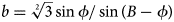 adjusts for the octahedral bulges on the area of contact. The square root of A contact is used as a width scale for the grain-to-grain contact for heat flow. The pore spaces themselves are truncated octahedrons with depressed, instead of bulged, faces.
Equations (A1–A7) can be used to calculate other needed geometric relations in terms of the size of the truncating cube, c, and either V 0 or ρ firn.
Appendix B. Thermal diffusivity
The thermal parameters of the firn controlling heat flow are thermal conductivity and thermal diffusivity. Thermal values for ice apply to the individual grains, but the bulk firn properties are due to the mixture of ice grains and air in the pores. The primary unknown is the bulk thermal conductivity K, since diffusivity is the bulk conductivity divided by the bulk density (ρ firn) and heat capacity of the firn grains. There is extensive literature concerning snow thermal conductivity, but most of those studies focused on low density snow. There are fewer estimates for high density firn. Cuffey and Paterson (Reference Cuffey and Paterson2010) suggest two empirical parameterizations: the Van Dussen formula:

and the Schwerdtfeger formula:

In previous research in our study area, Cox and others (Reference Cox, Humphrey and Harper2015) found the Schwerdtfeger formula gave a better match to field-measured temperature variations in the firn column. We bias our choice toward the Schwerdtfeger formula and use a single diffusivity of 10−6 m2 s−1 in our thermal calculations related to the perched aquifer.


 Open access