

1. INTRODUCTION
Dry snow slab avalanches are observed to release by propagating fractures in thin weak layers underneath cohesive snow slabs. The propagating disturbances are interpreted as shear fractures (McClung, Reference McClung1979, Reference McClung1981; Schweizer and others, Reference Schweizer, Jamieson and Schneebeli2003). Since dry snow slab avalanches are observed to initiate by propagating fractures within the weak layer, it is natural to apply fracture mechanics to the problem. There are two aspects to the problem which are very important. The first of these is to provide a framework for understanding the physical mechanism for avalanche release and this leads to the conclusion that avalanche prediction is a risk or probabilistic-based activity. Application of fracture mechanics to alpine snow shows that slab avalanches occur on the basis of failure of weak zones within the weak layer which are of macroscopic size (Bažant and others, Reference Bažant, Zi and McClung2003). These weak zones cannot generally be found and their properties cannot be measured. This constitutes the residual risk in avalanche forecasting which cannot be eliminated (McClung and Schaerer, Reference McClung and Schaerer2006; McClung, Reference McClung2011a).
The second aspect for application of fracture mechanics to avalanche formation has received much less attention. The second aspect is concerned with whether the application of fracture mechanics can help to forecast avalanches. Our paper is concerned with this second aspect. Our paper is based on the application of probabilistic methods combined with field measurements consistent with the experimentally verified mechanical and fracture properties of alpine snow.
Conventional fracture mechanics was developed by Griffith (Reference Griffith1920, Reference Griffith1925) nearly 100 years ago for brittle materials such as glass. It is termed: linear elastic fracture mechanics (LEFM). LEFM contains two important assumptions: (1) that the fracture process zone (FPZ) at the tip of the crack where failure is taking place is infinitesimal and (2) the material is linear elastic (rate-independent). Neither of the two important brittle fracture assumptions apply accurately to alpine snow in natural slab avalanche initiation (Mellor, Reference Mellor1968; McClung, Reference McClung2015). Alpine snow, in which avalanches form, is not a brittle material. It is found within 90% of the melt point and the volume fraction of ice is typically ~20% (or equivalently 80% air). Instead, alpine snow is termed quasi-brittle with respect to fracture since it has a finite-sized FPZ and it is highly rate-dependent. Quasi-brittle fracture mechanics has been experimentally verified to apply to alpine snow by hundreds of laboratory tests (Sigrist, Reference Sigrist2006; Borstad, Reference Borstad2011). The quasi-brittle character of alpine snow implies that there is a fracture mechanical size effect law on snow strength: larger specimens have lower strength than smaller ones. Bazant and others (Reference Bažant, Zi and McClung2003) provided a fracture mechanical size effect law on snow strength and applied it to avalanche release.
Our paper is concerned with a probabilistic formulation of a size effect law consistent with quasi-brittle fracture mechanics but compatible with a risk basis for avalanche forecasting. Our size effect law is based on a set of field-measured critical lengths, instead of snow strength. However, it applies to fracture initiation in weak layers consistent with the original fundamental basis of brittle fracture mechanics by Griffith (Reference Griffith1920, Reference Griffith1925). Since our analysis is probabilistic, rather than mechanical, the constraints necessary for application of LEFM such as linear elasticity are avoided.
Brittle fracture strength data have also been analyzed probabilistically (e.g. Freudenthal, Reference Freudenthal and Liebowitz1968). Weibull (Reference Weibull1939, Reference Weibull1951) showed that larger samples in tension are weaker than smaller samples with a probability density function (pdf) describing the effect given by a distribution which bears Weibull's name. The idea is that a larger sample has a higher probability of having a weaker flaw to produce earlier failure under loading. Bažant and Planas (Reference Bažant and Planas1998) and Bažant (Reference Bažant2005) have discussed the application of the Weibull brittle fracture theory to quasi-brittle materials and they have listed serious objections to the application of the theory. First, snow is not a brittle material. In addition, the scaling law of Weibull theory (Bažant, Reference Bažant2005) is scale invariant but with no characteristic length but this is not true for snow by the experiments of Sigrist (Reference Sigrist2006) and Borstad (Reference Borstad2011). Their experiments showed that a macroscopic FPZ implies a deterministic size effect which is different from that in the Weibull theory.
Quasi-brittle fracture is expected to follow the principle since a smaller crack in a sample should result in higher strength than one with a larger crack (Bažant and Planas, Reference Bažant and Planas1998). A sample with a crack size not much larger than the FPZ should have very high strength, while a longer crack should approach the low-strength limit required for LEFM where the crack length is much greater than the FPZ. A fundamental difference in the approaches of Weibull and quasi-brittle fracture is that Weibull is purely statistical, whereas quasi-brittle is a fracture mechanical formulation. Our formulation is probabilistic but it is consistent with quasi-brittle fracture mechanics.
In addition to the probabilistic size effect law, the paper contains an Appendix which helps illustrate the relationship of the probabilistic size effect law to the fracture mechanical strength size effect law of Bažant and others (Reference Bažant, Zi and McClung2003). We have also included information about how the new probabilistic size effect law might be used in practice.
2. BASIC FRACTURE MECHANICS, AVALANCHE FORMATION AND ALPINE SNOW
The development here is related to avalanche initiation involving fracture mechanics. The important quantities in fracture mechanics are bound together in the quasi-static energy equation:  $K_i = \sqrt {E{\rm ^{\prime}}G_i} $ (Irwin, Reference Irwin1958) where i denotes mode of loading taking values: I, II, III (in-plane tension, in-plane shear, anti-plane shear) in this paper. The parameter K i is the stress intensity factor containing the driving stress at the crack tip (units: Pa(m)1/2) and G i is the fracture energy: the energy to create a unit area of fracture surface (units: N/m or J/m 2). The reader is referred to Rice (Reference Rice and Liebowitz1968) and Tada and others (Reference Tada, Paris and Irwin2000) for more information. The modulus is: E′ = E/(1 − ν 2) (plane strain) or E′ = E (plane stress) where E, ν are the Young's modulus and Poisson's ratio. For the viscoelastic case, 1/E′ is replaced by the viscoelastic compliance in plane strain tension (Rice, Reference Rice1973; McClung, Reference McClung2015).
In this paper, we distinguish between the loading form which is in terms of the applied stresses and the fracture pattern which is observed (Rao and others, Reference Rao, Sun, Stephansson, Li and Stillborg2003). The loading form may be described using descriptive terms such as shear loading or compressive loading. The term fracture mode here refers to the observed fracture pattern. The loading is characterized by stress intensity factors (K I, KII, K III), whereas the mode of fracture is determined by observation of how the crack propagates. Formulation of stress intensity factors is beyond the scope of this paper.
At critical conditions just before self-propagation, the symbols: K Ic, K IIc are used to denote the fracture toughness associated with the observed fracture mode. The fracture toughness normally includes the critical length beyond which dynamic fracture occurs and the applied driving stress load. The third fracture mode (III) (anti-plane shearing) is observed under three-dimensional dynamic conditions in avalanche release (McClung, Reference McClung2009a). However, in this paper, only quasi-static conditions for in-plane conditions are analyzed, so mode III is discussed but not analyzed.
For the case of natural dry-slab avalanche release, the loading consists of compression and shear on the weak layer by the slab weight. However, the fracture propagates within the weak layer for distances on the order of 10s to 100s of meters. There is no observed kinking or branching up into the slab until the tensile fracture line appears on the order of 50 slab depths upslope (McClung, Reference McClung2009a). Observationally, the initial fracture is mixed mode II (in-plane: upslope) and III (anti-plane: across slope) within the weak layer which persists until the tensile fracture line forms far upslope under rapid, dynamic conditions. Figure 1 shows a dry-slab avalanche in the initial stages of motion released by explosive control. When combined with field observations, which show the fracture to propagate upslope and across slope from the initiation area, Figure 1 suggests that the fracture propagated upslope (mode II) and across slope (mode III) within the weak layer to produce tensile failure at the crown.
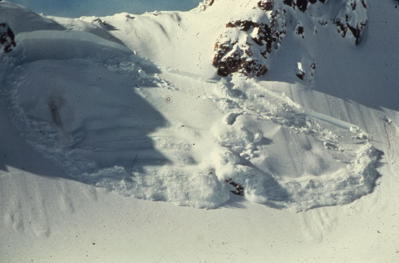
Fig. 1. Dry-slab avalanche in the initial stage of motion initiated by explosive control. The weak layer fracture spread upslope (mode II) and across slope (mode III) to cause tensile fracture at the crown. Photo by: T. Salway.
Our data were obtained from propagation saw tests (PST) (Gauthier, Reference Gauthier2007; Gauthier and Jamieson, Reference Gauthier and Jamieson2008b) by cutting a notch in the weak layer under a slab until a critical length L(m) was achieved resulting in rapid propagation within the weak layer. For the PST data (Fig. 2), the fracture is observed to propagate (in-plane) within the weak layer with no kinking or branching into the slab above or material below so the mode of fracture is called mode II. For PST, the sample width is 30 cm, so mode III is not evident.
Fig. 2. Schematic representation for the propagation saw test (PST). The cut is made within the weak layer starting from the free surface. The block is 30 cm wide and long enough that the end of the critical cut length (L) is not close to the end of the block. Typically, the block length is 1 m or more. In the figure, 2c f is the size of the fracture process zone.
In order to initiate and propagate fractures, an energy-based model is required. Several energy-based models are available at present. The model of Palmer and Rice (Reference Palmer and Rice1973) is based on quasi-static shear fracture (mode II) initiation within the weak layer (McClung, Reference McClung1979, Reference McClung1981, Reference McClung2015). Another is from Heierli and others (Reference Heierli, Gumbsch and Zaiser2008) which requires a macroscopic void in the weak layer. This paper is concerned with natural slab avalanche release using probabilistic methods, so detailed analysis of energy-based models is beyond the scope here.
A quasi-brittle, fracture mechanical size effect law on weak layer strength was proposed by Bažant and others (Reference Bažant, Zi and McClung2003) and is compatible with the model of Palmer and Rice (Reference Palmer and Rice1973). The quasi-brittle character of alpine snow was verified by hundreds of beam bending tension fracture tests in the Ph.D. theses of Sigrist (Reference Sigrist2006) and Borstad (Reference Borstad2011). Estimates of the size of the FPZ are typically in the range 2–10 cm (Sigrist, Reference Sigrist2006; Borstad, Reference Borstad2011).
3. DATA DESCRIPTION AND CHARACTERISTICS
The dataset was collected in the Columbia Mountains of eastern British Columbia. The dry snow avalanche stratigraphy (planar, cohesive slab over thin weak layer) was recognized by examining snow pits and from simple instability tests (e.g. McClung and Schaerer, Reference McClung and Schaerer2006) to reveal the slab/weak layer combinations.
The data were obtained from field-measured weak layer shear fracture tests (PST) (Gauthier, Reference Gauthier2007). The measurements were from the Ph.D. thesis of Gauthier (Reference Gauthier2007): Gauthier and Jamieson (Reference Gauthier and Jamieson2008a) as well as our own personal collection. They consisted of 591 tests for 45 slab/weak layer combinations. The tests were conducted by cutting a notch within the weak layer underneath a slab until the critical length L was reached and slope parallel, rapid propagation was achieved. Figure 2 contains a schematic representation of the test geometry. The data consisted of  $L,D,\psi, \bar{\rho} $ where $D,\psi, \bar{\rho} $ are: slab depth, slope angle and mean slab density. Weak layer crystal forms and size were also recorded for most tests. On average, more than ten tests were done to record a median value of L for each slab/weak layer combination. Each slab/weak layer combination is different. Therefore, analysis of the dataset does not yield results like laboratory tests where similar or nearly identical samples can be tested. Instead, the analysis yields only trends for the dataset as a whole. Table 1 contains basic descriptive statistics for the measurements and Table 2 has percentile values for L. Figure 3 is a dot histogram of the 45 critical lengths.

Fig. 3. Dot histogram of critical lengths. The range is: 0.07 m ≤ L ≤ 0.61 m with mean:  $\bar{L} = 0.30\,{\rm m}$.
Table 1. Descriptive statistics for PST from 45 slab–weak layer combinations (591 tests)
Table 2. Percentile values for L
By cutting a notch with a snow saw, we suggest that slope parallel and slope perpendicular displacement are produced in the weak layer and potential energy is released during unloading by slab motion in combination with weak layer deformation. The process eventually leads to the observed upslope propagation in the weak layer which is interpreted as the mode II weak layer fracture. The slope perpendicular displacement from the saw cut is compressive so it alone cannot drive the fracture in the slope parallel (upslope) direction as observed (McClung and Borstad, Reference McClung and Borstad2012a). Measurements of slope normal slab displacement prior to propagation (McClung and Borstad, Reference McClung and Borstad2012a) showed that it produces minor slab bending unless a thick snow saw is used.
An important limitation of the PST is that the weak layer must be thick enough (~1 cm) such that the saw can be guided through the layer without intersecting the slab above or the material below. We have observed avalanches to release on new, stellar crystals on the order of 1 mm thick. Avalanches have also been observed on surface hoar (≈1 mm thick) and facet layers (≈1 mm thick) over ice crusts and facet layers alone (≈1 mm thick) (Personal communications: D. Cochrane, K.Wyss, and C. Israelson: senior mountain guides). For all four such cases, PST would not be appropriate. Our field measurements have consistently shown that, without a sufficiently cohesive slab above, shear fracture propagation within the weak layer is not observed for PST.
As with any material test, PST must be interpreted carefully to yield information relevant to avalanche release. Natural dry-slab avalanches are observed to initiate by mixed mode II and mode III fracture in the weak layer for slope angles in the range: 25−55° (McClung, Reference McClung2013), whereas PST give mode II fracture results for any slope angle, even for ψ = 0°.The same is true through human intervention (skiing or walking) for ψ = 0°, propagation is sometimes observed which implies a positive weak layer driving stress and deformation along the weak layer both of which are not present under slab weight alone (McClung, Reference McClung2011b). Thus, the stress and deformation conditions for PST and human intervention are not the same as for natural avalanche release. For the PST, the increasing weak layer shear strain and stress as the saw is moved (under constant slab load) help initiate the mode II fracture (McClung, Reference McClung2015). Since the experiments showed that weak layer propagation takes place even for ψ = 0°, it is not possible that gravitational stresses alone drive the fracture unlike natural dry-slab release.
The dataset took ~10 field seasons to acquire and this type of dataset is probably unique in nature among mode II critical lengths measured in the field. Similar datasets were analyzed by Schweizer and others (Reference Schweizer, Reuter, van Herwijnen, Gauthier and Jamieson2014) and van Herwijnen and others (Reference van Herwijnen2016). No comparable dataset exists for earthquakes, landslides, ice or rock. The data are from different slab–weak layer combinations with slab depth, density and slope angle variations commonly found in avalanche applications. We performed Spearman rank correlation calculations for  $L,\bar{\rho}, D,\psi $. We found that L has significant positive correlation with D (0.61; p < 0.0005) but we found no other statistically significant correlations among directly measured variables. Rank correlation of L with the depth averaged slope perpendicular normal stress: $\sigma = \bar{\rho} gD\cos \psi $ gave 0.64 (p < 0.0005) and with the depth averaged slope parallel shear stress: $\tau = \bar{\rho} gD\sin \psi $ gave 0.60 (p < 0.0005) where g is the magnitude of gravity acceleration. The significance (p) for Spearman rank correlation, r s, was calculated from the t-statistic (Harnett, Reference Harnett1975) as: $t = r_{\rm s}\sqrt {(N-2)/(1-r_{\rm s}^2 )} $ with N − 2 as the number of degrees of freedom and use of tables of t to estimate p with significance defined as p < 0.05.
We also performed t-tests for the mean of L in relation to two groups of weak layer crystal forms: persistent forms (surface hoar, facets, depth hoar) and non-persistent forms (decomposing and fragmented). We found that the means of L are significantly different (p = 0.004) between the two groups: persistent forms compared with non-persistent forms. The persistent forms imply longer values of L. The longer values of L for persistent forms could result from the generally larger grains normally found in comparison to non-persistent (McClung and Schaerer, Reference McClung and Schaerer2006). Bažant and Planas (Reference Bažant and Planas1998) showed that the FPZ tends to increase with grain size for quasi-brittle materials which can imply longer critical lengths.
Another, more likely, possibility is that the persistent forms tend to last for longer periods in the snowpack. The strength and fracture toughness of surface hoar layers increase with time to ensure longer cut lengths L. We tracked surface hoar layers using the blade hardness gauge (Borstad and McClung, Reference Borstad and McClung2011) which correlates with tensile (mode I) fracture toughness and layer stiffness. For sets of measurements over 2 months, the results showed layer stiffness/fracture toughness increased by ~210% in one case and 970% after 1 1/2 months in another case (Pogue and McClung, Reference Pogue and McClung2016). For the same time frame, non-persistent layers normally bond and they do not display instability for such long periods. The increase of L with weak layer age is also compatible with the positive rank correlation of L with D since with as time passes weak layers should be buried more deeply from snow falls.
A related and very important source of information comes from slope angle results. For PST done on the same day at different slope angles (McClung, Reference McClung2009b), the critical cut length can be significantly shorter for ψ = 0° than for ψ ~30°. A simple explanation is that the saw cut produces both slope normal and slope parallel weak layer deformation by loss of gravitational potential energy from the slab motion even for ψ = 0°. McClung (Reference McClung2015) suggested that more slope normal displacement (low slope angle) also implies more slope parallel displacement and a shorter cut length (L). However, weak layer deformation has not been reported for PST. The slope parallel (shear) deformation also implies a positive weak layer shear stress term. The slope normal deformation alone cannot help drive the fracture in the slope parallel direction since it is working to close, not open the weak layer crack. Birkeland and van Herwijnen (Reference Birkeland and van Herwijnen2016) showed a related effect: added load for the same slope angle produces a shorter critical length.
Reiweger and Schweizer (Reference Reiweger and Schweizer2010, Reference Reiweger and Schweizer2013) measured the weak layer deformation components for surface hoar, facets and depth hoar in the laboratory. Their measurements showed shear strain localization within the weak layer with ~90% of the system deformation concentrated in the weak layer instead of the slab.
The slope angle results (McClung, Reference McClung2009b), the load results (Birkeland and van Herwijnen, Reference Birkeland and van Herwijnen2016) and the highly significant positive correlation (0.64) of L with σ suggest that there are two important timescales for PST. For the same day or over short timescales for the same or very similar slab and weak layer, the slope angle and load results (Birkeland and van Herwijnen, Reference Birkeland and van Herwijnen2016) show that L can decrease strongly as ψ decreases (or σ increases). Both of the added load and slope angle effects are on a short timescale. On the other hand, the correlation results for the entire data base show that L increases with D or σ (opposite to the short-term behavior) but no significant correlation with ψ, which we attribute partly to aging effects for the persistent forms which constitute most of the data base (or increase in K IIc).
Another important feature of PST, if they are to be of most use in describing avalanche release, is that the saw used should be as thin as possible. The reason is that a thick saw produces a void or hole, which is an artifact of the saw cut, to produce slab bending. For a PST, our observations have shown the observed weak layer fracture is always mode II with propagation observed within the weak layer and with no kinking or branching into the slab from the weak layer. However, use of a thick saw can produce excess slab bending causing slab tensile fracture ~1 D upslope from the end of the saw cut. We filmed the slab fractures (300 fps) and we found the slab fractures initiated at the top of the slab. This is not a mixed mode observed fracture condition since there are two separate cracks. Observation of mixed mode in fracture mechanics (Bažant and Planas, Reference Bažant and Planas1998; p. 95) refers to change in direction (kinking or branching) from a single crack. Thus, for a thick saw or low-density slab snow, slope parallel propagation (mode II) can occur along with an artificial tensile slab fracture (McClung and Borstad, Reference McClung and Borstad2012a; Schweizer and others, Reference Schweizer, Reuter, van Herwijnen, Gauthier and Jamieson2014; McClung, Reference McClung2015). The PST data reported here were all done with saw thickness ≤2 mm. Since the saw thickness is often comparable to the weak layer grain size, a crack made for a PST must be considered blunt at the tip and any conclusions about weak layer fracture properties using fracture mechanics must be regarded as approximate at best.
The slab fractures which do occur in PST are very near to the end of the saw cut (within about one slab depth, D upslope) and they appear unrelated to the tensile failures that are observed in the formation of the crown in avalanche release (Fig. 1), which are typically ~50 D upslope of the weak layer initiation point (McClung, Reference McClung2009a) and under fully dynamic conditions. Perla and LaChapelle (Reference Perla and LaChapelle1970), Perla (Reference Perla1971) and McClung and Schweizer (Reference McClung and Schweizer2006) predicted that the tensile fractures at the crown in avalanche release originate near the bottom of the slab from shear fractures.
4. PROBABILITY ANALYSIS OF THE DATASET
Analysis was performed to find the best-fitting pdf for the 45 values of L. The analysis was done for 65 distributions with a fit found for 60. The best-fitting distribution was found to be a gamma distribution based on the results of five goodness-of-fit tests. The tests included the Kolmogorov–Smirnov (K-S), Anderson–Darling (A-D) and χ 2 (C-S) statistics plus Q-Q (quantile) and P-P (probability) plots. The choice of the gamma distribution was made on the basis of preference of a two-parameter distribution over more complicated distributions of three and four parameters. For the gamma distribution, the statistics were (critical values for the significance parameter: α = 0.2 in parentheses): K-S: 0.09 (0.16); A-D: 0.37 (1.37); C-S: 2.9 (6.0). The higher the value of α is, the lower the critical values are, to yield a more stringent condition on the fit. The three-parameter gamma distribution yielded nearly identical fit statistics to the chosen two-parameter gamma distribution but it introduces added complexity.
For the gamma distribution, the scale parameter was L 0 = 0.05 m and the shape factor: n = 5.92 ≈ 6. The gamma pdf is given by:
 $$f\,(L) = \displaystyle{{L^{n-1}} \over {L_0^n \Gamma (n)}}\exp \left( {\displaystyle{{-L} \over {L_0}}} \right),$$
where Γ(n) is the gamma function.
A very good fit was also found for the Weibull distribution. For the Weibull distribution, the statistics (α = 0.2) were: K-S: 0.09 (0.16); A-D: 0.43(1.37); C-S: 6.0 (6.0). The Weibull distribution passed the C-S at α = 0.1 where the critical value was 7.8. The Weibull distribution had Weibull modulus (shape parameter) m = 2.57 and scale parameter: 0.34 m. Of the extreme value distributions (Weibull, Gumbel, Fréchet, Generalized), the Weibull provided the best fit but it was not quite as good as the gamma distribution. Since our paper applies to natural avalanche release for which ψ ≥ 25°, we repeated the calculations for that condition (36 slab-weak layer combinations; 443 tests). The distribution parameters for the gamma pdf were: L 0 = 0.05 m; n = 6.1 and for the Weibull pdf, they were: m = 2.76; scale parameter: 0.34 m.
The skewness calculated from the data is: 0.48 (sample size 45). The skewness for the gamma distribution is:  $2/\sqrt n = 2/\sqrt 6 = 0.82$ and for the Weibull distribution with m = 2.6 it is: 0.32 (Rousu, Reference Rousu1973) where both of the latter values imply infinite sample size. Thus, the data skewness lies between the theoretical values of the two distributions.
For the gamma distribution, the mean  $\bar{L} = (n)L_0 = 6(0.05) = 0.30\,{\rm m}$ (vs 0.31 m from the data), the most probable value (mode) is (n − 1)L 0 = 5(0.05) = 0.25 m and the Std dev. is: σ st = (n)1/2L 0 = 0.12 m (vs 0.13 m from the data). Figure 4 is a quantile plot (Q-Q plot) for L(m) measured (ordinate) vs. L(m) calculated from the inverse of the gamma function. The regression line had adjusted coefficient of determination: R 2 = 0.99.
Fig. 4. Quantile–quantile plot: L(m): measured vs L(m): model for the gamma distribution.
5. PROBABILISTIC MODEL FOR MODE II CRITICAL LENGTHS
Bažant (Reference Bažant2004) formulated a probabilistic strength framework for quasi-brittle materials and McClung and Borstad (Reference McClung and Borstad2012b) applied probabilistic methods to the strength of alpine snow.
Here, a probabilistic model for the measured critical fracture lengths by PST is derived. The model consists of dividing the length L (per unit width) into small representative linear elements (RLE) of length equal to c f (half the length of the FPZ) (Bažant and Pang, Reference Bažant and Pang2006, Reference Bažant and Pang2007) for mode II fracture in the weak layer (Fig. 2). From Sigrist (Reference Sigrist2006) and Borstad (Reference Borstad2011), the mean value  $\bar{c}_{\rm f} = 0.02\,{\rm m}$ based on 143 tensile laboratory beam bending tests. There are no values available from shear tests, so the tensile data are relied upon here. We expect the recorded cut length (L) to be a very good approximation of that shown in Figure 2. Once propagation is sensed, it takes a short amount of time to stop the saw cutting which implies the recorded length includes a few centimeters extra which is approximately the same as c f.
Each RLE is deemed too small to cause fracture of the layer itself but traversing the weak layer with the saw causes a crack to form, which weakens the system (slab + weak layer). The longer the crack, the weaker the system which implies a size effect based on measured length L to cause fracture. Each RLE is small and governed by a small size, constant high strength value  $(\tau_0^{\ast})$ considered to fail in a plastic (or size-independent) manner when the applied stress ratio: $\tau /(\tau_0^{\ast})$ at a suitable shear strain γ* produced by the saw cut. Plasticity here refers simply to constant yield stress, not that plasticity is being applied to model the snow. For the notation here (*) refers to properties of each small RLE assumed constant for the simplest model. Each RLE is characterized by a probability of fracture P* and a Weibull modulus m (Weibull, Reference Weibull1939, Reference Weibull1951) which represents an index of the number of micro-fractures in an RLE (Bažant and Pang, Reference Bažant and Pang2006, Reference Bažant and Pang2007). From McClung and Borstad (Reference McClung and Borstad2012b), it is assumed P*−1/m; m ≥ 1 as the conditional density of micro-fractures for each RLE. If m = 1, an RLE sustains only one micro-fracture and its probability of survival is zero for the next micro-fracture. When m is large, the material can survive many micro-fractures within an RLE and its probability of survival increases when m micro-fractures can be sustained prior to fracture. For any quasi-brittle material such as snow, m >1.
As an initial, simple model, we assume the weak layer consists of many identical RLEs. All RLEs have the same conditional density of micro-fractures. The survival probability for one RLE is: 1 − P*. As the saw cut is lengthened, the system becomes weaker and the overall survival probability decreases. For finite N individual RLEs cut in succession, the probability of survival, for the system is: P S = 1 − P F, is (Bažant and Planas, Reference Bažant and Planas1998):
 $$\eqalign{1-P_F & = (1-P{^\ast})(1-P{^\ast}) \ldots (1-P{^\ast}) \cr & = (1-P{^\ast})^N = {\rm e}^{N{\rm ln(1}-P{^\ast})}}.$$
Given that P*must be small, ln(1 − P*) ≈ P* and with N = L/c f, we arrive at:
 $$\eqalign{P_{\rm F} & = 1-\exp -\displaystyle{{LP{^\ast}} \over {c_{\rm f}}} \cr & = 1-\exp -\displaystyle{L \over {c_{\rm f}m}} = 1-\exp \left( {-\displaystyle{L \over {L_0}}} \right).}$$
In (3), 1/L 0 = 1/(m c f) is an average linear concentration of material fracture probability (units per meter).
Equation (3) is basic and it relates P F to the length L for the first occurrence of a Poisson event (Benjamin and Cornell, Reference Benjamin and Cornell1970). It contains the elements of fracture and size effect. As L → 0, P F → 0 which implies low probability of failure, and small size, high strength plastic failure. As L becomes large, P F → 1 which implies low strength and large size with crack length much greater than the FPZ size (2c f). Thus, for large enough, L, from a fracture mechanics perspective, the system approaches the condition of LEFM which implies L ≫ c f (Appendix A).
Application of Eqn (3) with the PST for the mean of the data ( $\bar{L} = 0.31\,{\rm m}$) for the exponential distribution yields L 0 = 0.31 m and m = 15.5 (with c f = 0.02 m). The estimated value of m is much too high for alpine snow and it exceeds the best estimate for concrete:m = 12 (Bažant and Planas, Reference Bažant and Planas1998). In addition, the initial simple model (Eqn 3) does not match the data. For L = 0.10 m P F = 0.21 which is much too high based on the descriptive statistics for the data (Table 2) which give a cumulative value P F = 0.05. The conclusion is that the implied value of L 0 is too high from this simple model. The next section contains a refined analysis to correct these deficiencies with connection to the observed gamma distribution.
6. THE GAMMA DISTRIBUTION FOR MODE II CRITICAL LENGTHS L
Equation (3) can be recognized as the spatial encounter probability for Poisson events: the probability that at least one event can cause fracture with Poisson parameter: L/L 0:
 $$P_{\rm F} = 1-\exp \left({-\displaystyle{L \over {L_0}}}\right) = \exp \left({-\displaystyle{L \over {L_0}}}\right)\sum\limits_{k = 1}^{\infty}{\displaystyle{1 \over {k!}}} \left({\displaystyle{L \over {L_0}}}\right)^k.$$
Freudenthal (Reference Freudenthal and Liebowitz1968) derived the same expression for statistical brittle fracture from purely probabilistic means without the use of mechanics with L referring to sample size (length) instead of crack length.
An ‘event’ is defined from the damage incurred by traversing a length such that the minimum critical length for fracture is realized. This length is close to the size of the FPZ ≈ 2c f. Instead of at least one event potentially causing fracture, fracture is considered associated with N prior damage events with fracture potentially occurring on the next event(n + 1). Eqn (4) is then replaced by (Freudenthal, Reference Freudenthal and Liebowitz1968; Olkin and others, Reference Olkin, Gleser and Derman1980):
 $$\eqalign{P_{\rm F}(L) & = \exp \left( {-\displaystyle{L \over {L_0}}} \right)\sum\limits_{k = n}^\infty {\displaystyle{1 \over {k!}}} \left( {\displaystyle{L \over {L_0}}} \right)^{k} \cr & = 1-\exp \left( {-\displaystyle{L \over {L_0}}} \right)\sum\limits_{k = 0}^{n-1} {\displaystyle{1 \over {k!}}} \left( {\displaystyle{L \over {L_0}}} \right)^k},$$
which implies fracture is associated with at least N independent prior events in succession. Eqn (5) represents the cumulative probability of fracture for a gamma distribution with Nas an integer (the Erlang distribution). In (5), the formalism L 0 = mc f is retained from physical principles as above. The Weibull modulus calculated from the data was m = 2.57 which gives: L 0 = c fm = (0.02)(2.57) = 0.05 m in agreement with the calculated value for the gamma distribution. The near-perfect agreement is fortuitous since c f is expected to vary with density (Sigrist, Reference Sigrist2006) and/or grain size (Borstad, Reference Borstad2011).
Differentiation of (5) with respect to L yields the gamma pdf. Physically Eqn (5) represents irreversible cumulative damage as the saw traverses a number of damage events (about the size of the FPZ or two RLE). Each event is too small to cause fracture (very low P F). Eqn (5) predicts P F = 0.0006 for L = L 0 = 0.05 m. Each RLE is characterized by high strength in the plastic limit $(\tau_0^{\ast})$, a length c f and Weibull modulus m representing an index number of micro-fractures over the distance c f (Bažant and Pang, Reference Bažant and Pang2006, Reference Bažant and Pang2007).
In the probabilistic size effect law, P S is a proxy for strength. Figure 5 contains the probabilistic size effect law with a log–log plot of the probability of survival based on the measured lengths: P S = 1 − P F vs L/L* for 0.07 m ≤ L ≤ 0.61 m; L* ≃ L 0 = 0.05 m. The symbol L*, as roughly equivalent to L 0, is derived in Appendix A from the strength size effect law of Bažant and others (Reference Bažant, Zi and McClung2003) compatible with the PST data. The probability of survival is mathematically equivalent to an exceedance probability. The values of P S were calculated from the gamma distribution with the PST data: P S = 1−I(n, β); L* = 0.05 m;n = 6 where I(n, β) is the incomplete gamma function and L/L* = β. For integer n, the survival probability, P S(β, n), is then from Eqn (5):
 $$P_{\rm S}(n,\beta ) = \left( {1 + \beta + \displaystyle{{\beta^2} \over {2!}} +... + \displaystyle{{\beta^{n-1}} \over {(n-1)!}}} \right){\rm e}^{-\beta}. $$
Fig. 5. Log–log plot of probability of survival: P S vs L/L*.
Appendix A contains the empirical fracture mechanical strength size effect law for dry-slab avalanche initiation by Bažant and others (Reference Bažant, Zi and McClung2003). Figures 5 and 6 (Appendix A) represent a companion pair of size effect laws which are conceptually very different. Figure 6 represents a case derived for a crack already in place, whereas Fig. 5 represents a sample for which a notch is cut. In both cases, L represents about half the total crack length for the scenario of avalanche release (Bažant and others, Reference Bažant, Zi and McClung2003; McClung, Reference McClung2011a; McClung, Reference McClung2015). Figure 6 is derived empirically from fracture mechanics with matching to plasticity (small size) and LEFM (large size) limits. Figure 5 is developed entirely from analysis of field and laboratory data.
Both size effect laws apply to quasi-brittle fracture. For example, the probabilistic size effect law predicts P S ≈ 1 for crack lengths less than or equal to the size of the FPZ. Both contain the same fundamental length scales L and L 0, L* with the latter two being approximately equal and close to the FPZ size ~2c f. For the brittle fracture limit (Griffith, Reference Griffith1920, Reference Griffith1925), the FPZ is infinitesimal so it need not appear in a formulation. Freudenthal (Reference Freudenthal and Liebowitz1968) studied brittle fracture statistically from the perspective of sample size and the FPZ length does not appear. Here quasi-brittle fracture is analyzed statistically from the perspective of critical lengths and the FPZ appears as an important length scale.
Equation (6) may also be expressed directly in terms of the strength size effect law ((A2): Appendix A) by the substitution:  $\beta = \lpar {{{\tau_0^{\ast}} / {\tau_N}}} \rpar ^2-1$ to illustrate the non-linear relationship between the two size effect laws. From (6) as β → 0, P S(n, β) → 1 and if β ≫ 1, P S(n, β) → 0.
The plot (Fig. 5) shows very high P S for small L indicating the high strength plastic limit and low P S for large L approaching the condition within 4% (L/L* = 12.2) of the LEFM limit in the sense that L ≫ c f.
For both size effect laws, it is important to emphasize that snow is not generally an elastic material and, in particular, the PST are not elastic nor does LEFM strictly apply (McClung, Reference McClung2015). The LEFM limit, in this case, applies if L ≫ 2c f (or β ≫ 1) as in the original treatment of fracture (Griffith, Reference Griffith1920, Reference Griffith1925). The brittleness number (Bažant and Planas, Reference Bažant and Planas1998): β ≃ L/L* from the PST here had a median 7 and a range 1.4–12.2. Thus, many of the tests imply, from the perspective of the finite size: 2c f, that LEFM is, at best, a rough approximation for the data even if the rate condition on inapplicability of linear elasticity is ignored. The role of elasticity for the PST is explained in detail by McClung (Reference McClung2015).
7. PRACTICAL USE OF THE PROBABILISTIC SIZE EFFECT LAW
The critical length L(m) is easily measured in the field and the driving applied shear stress, τ, at the weak layer for natural avalanche release may be calculated. Since avalanches are observed to initiate by mode II fracture propagation, K IIc is of more interest than the weak layer strength and L is an important component of K IIc. Suggested values for K IIc for avalanches and PST have been given by McClung (Reference McClung2015).
For PST, a short value of L implies easy attainment of a fracture condition which implies a higher degree of instability than a longer value since more energy input is implied to generate an unstable fracture for the latter. More formally, a short critical length coupled with a low value of τ implies relatively low fracture toughness. Experience also suggests that if a dynamic propagating fracture is not observed during a PST, the situation is likely stable. In addition, a probabilistic formulation in terms of L, fits in well with risk analyses which are couched in terms of probability (McClung, Reference McClung2011a, Reference McClung2014). It is clear that either P F or P S represent conditional probabilities since a cohesive slab over the weak layer is needed in order to get a fracture to propagate.
With a crack in place (as may be encountered in backcountry travel), the strength size effect law implies lower strength for increasing length and the probabilistic law predicts lower probability of survival. Thus, for either law, higher instability is implied for a longer in situ crack or imperfection. However, when a PST is performed, a longer cut implies more energy had to be input to reach a fracture condition reflecting higher resistance to fracture and propagation.
If one was to use measured values of L as an approximate, partial component of fracture toughness, we suggest testing around the median value of our slope angles: ψ = 30° for future measurements. One could use either the percentile values (Table 2) to represent non-exceedance probabilities or the gamma distribution for more accurate results. Important values from Table 2 and the analysis include: L = 0.10 m (very short); L = 0.55 m (very long) and L = 0.25 m (most probable).
Gauthier and Jamieson (Reference Gauthier and Jamieson2008b) outlined a method to evaluate avalanche potential based on the dynamic characteristics of the fracture after initiation for the PST. It is expected that both the critical length prior to propagation, as analyzed here, and the dynamic characteristics after propagation (Gauthier and Jamieson, Reference Gauthier and Jamieson2008b) provide useful information in practice. Gauthier and Jamieson (Reference Gauthier and Jamieson2008b) correlated PST results with weak layer failure initiation and adjacent slope instability tests. They found best correlation with adjacent slope instability using the simple rule that high propagation potential and high slope instability were defined by short values of L (e.g. low fracture toughness) and dynamic propagation across the entire column length without arrest. The analysis in this paper provides a way to define quantitatively what is meant by a short value of L for their method and its link to K IIc. We suggest that purely stress-based methods of avalanche instability evaluation, such as the infinite slope model, be abandoned in favor of an energy-based approach which is needed to describe the observed initiation of mode II weak layer fracture.
8. CONCLUSIONS
1. Natural dry-slab avalanches are observed to initiate by mixed mode II (upslope) and III (across slope) fracture propagation in the weak layer. Figure 1 illustrates the II, III fracture modes for an avalanche generated by explosive control. For PST, the observed fracture propagation is mode II. Since both dry-slab avalanches and PST are observed to exhibit mode II propagation, the assumption is that both initiated as mode II. Since the PST samples have 30 cm width, mode III is not evident.
Observations along with PST show (Schweizer and others, Reference Schweizer, Reuter, van Herwijnen, Gauthier and Jamieson2014; McClung, Reference McClung2015) that use of a thick saw or low-density slab material or both, tensile fracture can occur at the top of the slab. In such cases, there are two cracks and this is not mixed mode fracture. In fracture mechanics, mixed mode fracture refers to kinking or branching at the tip of one crack (Bažant and Planas, Reference Bažant and Planas1998, p. 95). Instead for PST, artificial slab bending can occur and the sample may fracture in tension at the top of the slab just ahead of the saw cut which is not observed in avalanche initiation. In order that the PST are most relevant to avalanche release (mode II), we suggest thin saws should be used to minimize the bending caused by the saw cut.
2. For natural avalanche instability evaluation, K IIc is much more fundamental than any purely stress-based approach (McClung and Schaerer, Reference McClung and Schaerer2006, p. 80–81). Two of the important components of K IIc are directly measureable or calculated along with the PST for the simplest models: the critical length L and the depth averaged gravitational loading shear stress τ on the weak layer.
3. In practical usage of the PST, the observed dynamic propagation all along the weak layer and a short value of L correlate best with observed instability (Gauthier and Jamieson, Reference Gauthier and Jamieson2008b). The analysis in this paper provides a quantitative framework compatible with the known quasi-brittle fracture properties of alpine snow to define what is meant by a short value of L. The measured slope angle dependence of the tests (McClung, Reference McClung2009b) over short timescales is a disadvantage of using lengths from PST as indices of instability. However, tests at the same slope angle (e.g. ψ = 30°) may provide guidance about strength/fracture toughness and its increase with time.
4. Models based on yield stress, linear elasticity or LEFM cannot explain the known quasi-brittle fracture mechanical size effect for alpine snow. For conditions of natural dry-slab avalanche release, alpine snow is not linear elastic, nor does it follow LEFM (Mellor, Reference Mellor1968; McClung, Reference McClung2015). Measured shear strain rates in storm snow are ~10−7/s and about 10−8/s for well-settled snow (McClung, Reference McClung1974). In order to approach linear elasticity and rate independence, strain rates of about 102/s are required (Mellor, Reference Mellor1975; Sigrist, Reference Sigrist2006). Stress-based yield models are size-independent and analogous to plasticity (Bažant and Planas, Reference Bažant and Planas1998). A stress-based yield model was given by Reiweger and others (Reference Reiweger, Gaume and Schweizer2015). Chiaia and others (Reference Chiaia, Cornetti and Frigo2008) compared stress- and energy-based models. In this paper, models based on yield stress, linear elasticity, dynamics and LEFM could not be considered in the probabilistic size effect law development. However, that does not mean such models are not useful or important.
5. Tests from PST cannot be considered linear elastic since they exhibit temperature dependence (Reuter and Schweizer, Reference Reuter and Schweizer2012; McClung, Reference McClung1996; McClung, Reference McClung2015). The elastic modulus of the parent material (ice) varies only by ~5% down to −50°C (Schulson and Duval, Reference Schulson and Duval2009). In addition, the deformation rate during PST is too slow to justify linear elasticity (McClung, Reference McClung2015).
6. Tests from PST are not determined by gravitational slab weight loading alone in contrast to natural slab release(25° ≤ ψ ≤ 55°). The observed propagation from a PST or human triggering for flat terrain (ψ = 0°) is due to a complex pattern of deformation from human influence either by the saw cut (PST) or human motion (McClung, Reference McClung2011b). The observed slope angle dependence for PST done on over a short timescale (McClung, Reference McClung2009b) is artificial and cannot be directly related to natural avalanche release since the weak layer deformation and stress conditions are expected to be different and fracture is noted for low slope angles (even for ψ = 0°). Again, this is why we recommend performing the tests at the same or similar slope angles to compare results.
7. The size effect law based on L in this paper is built entirely from field and laboratory measurements from alpine snow and it does not have nearly the limitations of the strength size effect law of Bažant and others (Reference Bažant, Zi and McClung2003). However, the probabilistic size effect law is consistent with the strength size effect law. The use of survival probability as a proxy for shear strength fits naturally into risk analyses. Specifying a shear strength always requires a model combined with measurements to calculate the strength whereas L is easily measured directly.
8. The probabilistic model here is meant to be consistent with the known fact that alpine snow is a quasi-brittle material and the model is kept simple for practical application. In particular, the model does not include the expected, progressive stress redistribution as the saw cut is made. Introduction of stress redistribution into the model is beyond the scope here. The critical length measurements (Section 3) and the gamma distribution fit to the data (Section 4), based on five goodness-of-fit tests, should hold even if a more complex model involving stress is developed. The measurements should implicitly include any stress redistribution even though such is not explicitly included in the model.
9. Figures 5 and 6 represent two conceptually different situations probabilistically. With regard to strength, McClung and Borstad (Reference McClung and Borstad2012b) suggested that the shear strength of un-notched samples from avalanche weak layers follows a gamma distribution (Sommerfeld and King, Reference Sommerfeld and King1979) and the gamma distribution converges asymptotically to a Weibull distribution in the large size (low strength) limit, as it must (Bažant, Reference Bažant2005, p. 62). However, when the physical size becomes very large (as in an avalanche weak layer), the possibility of macroscopic imperfections increases. The system is then likely to be controlled by a deterministic type 2 energetic size effect law (Fig. 6). Figure 5 is meant to convey an index of the probability of fracture for the system based on PST measurements. Figure 6 is meant to display the deterministic behavior expected for avalanche initiation with a macroscopic imperfection in place for which the probabilistic distribution of strength is of less significance.
ACKNOWLEDGEMENTS
This work was funded by the Natural Sciences and Engineering Research Council of Canada and the University of British Columbia.
APPENDIX A
RELATION TO TYPE 2 ENERGETIC SHEAR STRENGTH SIZE EFFECT LAW
The presence of a notch or crack in a sample implies a type 2 energetic, fracture mechanical size effect for a quasi-brittle material (Bažant and Planas, Reference Bažant and Planas1998; Bažant, Reference Bažant2005) such as alpine snow. Bažant and others (Reference Bažant, Zi and McClung2003) gave an empirical quasi-brittle size effect law for nominal shear strength to represent the slab–weak layer system by asymptotic matching for between the small size plastic limit shear strength  $(\tau_0^{\ast})$ and the large size LEFM limit on the other extreme. The term plastic is meant to denote the small, size-independent limit of shear strength (Bažant and Planas, Reference Bažant and Planas1998) not that plasticity applies in alpine snow mechanics. The mode II size effect law, neglecting residual shear strength, is:
 $$\displaystyle{{\tau_N} \over {\tau_0^{\ast}}} = \displaystyle{1 \over {\sqrt {1 + (D/D_0)}}}.$$
 In (A1), τ N is the nominal (size-dependent) shear strength, D is the slab depth (Fig. 1) measured perpendicular to the plane of the slab–weak layer system and D 0 is a transitional size which represents an inflection point size for transition between the small size asymptote:  $D/D_0\to 0,\tau_N\to \tau_0^{\ast}$ and the large size limit D/D 0 ≫ 1(LEFM) with $\tau_N/\tau_0^{\ast}\propto 1/\sqrt D $.
For Eqn (A1) (Bažant and others, Reference Bažant, Zi and McClung2003), D 0 = 2c f/(L s/D − c f/D). In this expression, L s represents half the length of a crack embedded in a weak layer. However, the length measured(L) in a propagation saw test is shorter than that in the size effect law (Bažant and others, Reference Bažant, Zi and McClung2003; McClung, Reference McClung2015) since a free surface is present at the beginning of the cut (Fig. 1) with intact material beyond the end of the cut. This mismatch results in relief of longitudinal pressure (Palmer and Rice, Reference Palmer and Rice1973) to help promote fracture. McClung (Reference McClung2015) provided field measurements and analysis to give an empirical expression: L s = L + 0.1D to relate the lengths.
Substitution in (A1) yields an approximate equivalent strength size effect law:
 $$\displaystyle{{\tau_N} \over {\tau_0^{\ast}}} = \displaystyle{1 \over {\sqrt {1 + ((L + 0.1D-c_{\rm f})/(2c_{\rm f}))}}} \approx \displaystyle{1 \over {\sqrt {1 + (L/L{^\ast})}}},$$
where L* represents a transitional crack length (approximated as constant below) between small size plastic behavior (very small P F or high overall strength,  $\tau_0^{\ast}$) and large size LEFM behavior (very high P F and low nominal strength). If L < c f then $\tau_N = \tau_0^{\ast}$ (the small size plastic limit) and if L ≫ c f the LEFM limit is implied. For practical cases, it makes no sense to consider crack sizes smaller than c f so Eqn (A2) is considered for L ≥ c f.
Equation (A2) implies L* = 2c f/(1 + 0.1D/L − c f/L) which yields: 0.03 m< L* < 0.05 m (mean and median 0.04 m) for c f = 0.02 m; 0.07 m ≤ L ≤ 0.61 m as measured for the PST. For comparison of the size effect laws, the value: L* ≈ L 0 = 0.05 m is assumed here. With L* = 0.05 m, the approximation in Eqn (A2) holds well for L ≥ 0.12 m.
Either (A1) or (A2) are approximations which will not hold in the limit of very small cracks (Bažant and others, Reference Bažant, Zi and McClung2003). For Eqn (A2) the expression under the square root radical in the denominator is a result of a two-term Taylor series approximation (Bažant and others, Reference Bažant, Zi and McClung2003) with respect to: c f /D. The complete expression within the radical is: 1 + (L − c f)/2c f + c f /2(L − c f). If the second term is ≥25 times the third term, then it is implied that L ≥ 6c f which yields L ≥ 0.12 m for c f = 0.02 m. From Figure 3, this condition applies to 43 of 45 slab–weak layer combinations in the dataset or  $\tau_N/\tau_0^{\ast} \le 0.54$.
Figure 6 contains a schematic log–log plot for  $\tau_N/\tau_0^{\ast} \, {\rm vs} \, L/L^{\ast}$ for 0.02 m ≤ L ≤ 0.60 m with L* = 0.05 m. The figure shows the same form as the classical size effect law for mode II formulated by Bažant and others (Reference Bažant, Zi and McClung2003). The horizontal asymptote for plasticity is approached at small size and the Griffith (Reference Griffith1920; Reference Griffith1925) condition of LEFM is approached for large size (L): $\tau_N\sqrt L $ = constant. Thus, as with Eqns (A1) and (A2) represents proper asymptotic matching between the small and large size limits. The vertical line represents the approximate limit: L/L* = 2.4 below which the data here would not be accurate within the strength size effect approximation (Eqn A2) as explained by Bažant and others (Reference Bažant, Zi and McClung2003).
Fig. 6. Schematic log–log plot of strength ratio:  $\tau_N/\tau_0^{\ast}$ vs L/L*. The vertical line represents the limit on the abscissa: L/L* = 2.4 above which the calculations are approximately valid.
For rough comparison of the size effect laws (Fig. 5, (A1)), the scaling length was chosen as: L* = 0.05 m. For the strength size effect law (A2), the scaling length is: 2c f whereas for the gamma distribution it is the scale parameter (L 0). The two differ by only 1 cm under the assumptions in this paper. We believe the closeness of the two values is fortuitous. The value used for the comparison was chosen since it was derived from the PST, whereas the value of 2c f was estimated from lab tensile tests which show variations with density and rate (Borstad, Reference Borstad2011).


 Open access