


1. Introduction
Relatively thick and extensive debris cover on glacier ablation area is commonly found in many glacierized regions globally (Scherler and others, Reference Scherler, Wulf and Gorelick2018, Herreid and Pellicciotti, Reference Herreid and Pellicciotti2020). When this debris accumulates to a thickness of more than a few centimetres, it acts as an insulating layer for the underlying ice and slows down the melting rate (Østrem, Reference Østrem1959, Pratap and others, Reference Pratap, Dobhal, Mehta and Bhambri2015, Laha and others, Reference Laha2017, Rounce and others, Reference Rounce2021). While one might expect that an expanding and thicker layer of debris would reduce the thinning of debris-covered glaciers compared to the debris-free glaciers, this anticipated contrast in melt rates is not consistently observed in glacier-thinning data (Nakawo and Rana, Reference Nakawo and Rana1999, Zhang and others, Reference Zhang, Fujita, Liu, Liu and Nuimura2011, Anderson and others, Reference Anderson, Armstrong, Anderson, Scherler and Petersen2021b). This is termed as the ‘debris cover anomaly’, which has also been noted across the Himalaya (Vijay and Braun, Reference Vijay and Braun2016, Brun and others, Reference Brun, Berthier, Wagnon, Kääb and Treichler2017). This anomaly is explained by the evolution of emergence velocity (Banerjee, Reference Banerjee2017), the variability of debris thickness (Chen and others, Reference Chen, Wang, Li, Yang and Zhang2023) and the presence of transient features such as supraglacial ice cliffs and water bodies (e.g. ponds) (Brun and others, Reference Brun2018, Miles and others, Reference Miles, Willis, Buri, Steiner, Arnold and Pellicciotti2018, Reference Miles, Steiner, Buri, Immerzeel and Pellicciotti2022). An ice cliff is a steep or near-vertical face of exposed ice found on debris-covered glaciers. They are formed by several processes like englacial channel collapse, calving, crevassing and supraglacial streams causing erosion and differential melting where the insulating debris is thin or absent (Watson and others, Reference Watson, Quincey, Carrivick and Smith2017a, Steiner and others, Reference Steiner, Buri, Miles, Ragettli and Pellicciotti2019, Kneib and others, Reference Kneib2021). These ice cliffs often appear dirty due to the presence of thin supraglacial debris that may cover all or part of them (Sakai and others, Reference Sakai, Masayoshi and Fujita1998, Buri and others, Reference Buri, Pellicciotti, Steiner, Miles and Immerzeel2016b, Buri and Pellicciotti, Reference Buri and Pellicciotti2018). The lower albedo of these dirty ice cliffs leads to higher melting rates compared to the surrounding debris-covered ice (Sakai and others, Reference Sakai, Nakawo and Fujita2002, Steiner and others, Reference Steiner, Pellicciotti, Buri, Miles, Immerzeel and Reid2015, Kneib and others, Reference Kneib2023, Reference Kneib2022). It is clear that the melting regimes of debris-covered glaciers are complex, and the supraglacial ice cliffs play a critical role in local glacier surface energy- and mass-balance processes. These complex regimes are responsible for glacier topographic changes, ice cliff expansion, and the development of supraglacial ponds or lakes (Sakai and others, Reference Sakai, Takeuchi, Fujita and Nakawo2000, Brun and others, Reference Brun2018, Steiner and others, Reference Steiner, Buri, Miles, Ragettli and Pellicciotti2019).
Previous studies have reported that the ice cliff melt rates or thinning rates at ice cliff locations in the Himalaya on seasonal and annual time scales are higher compared to the adjacent glacier surface with continuous debris cover at similar altitudes (Sakai and others, Reference Sakai, Masayoshi and Fujita1998, Reid and Brock, Reference Reid and Brock2014, Brun and others, Reference Brun2016, Vincent and others, Reference Vincent2016, Buri and others, Reference Buri, Miles, Steiner, Ragettli and Pellicciotti2021, Kneib and others, Reference Kneib2022). For example, Brun and others (Reference Brun2016) applied structure from motion over a set of terrestrial images of Lirung Glacier, Nepalese Himalaya, and found six times higher seasonal mass loss rate at the ice cliff locations compared to the debris-covered part of the glacier. Similarly, Kneib and others Reference Kneib2022 employed a set of time-lapse camera systems at 24K and Langtang Glaciers and reported 4–14 times higher ice cliff melt rates compared to the surrounding debris-covered parts over the summer season.
While the seasonal to sub-seasonal backwasting of ice cliffs on individual Himalayan debris-covered glaciers is well constrained, short-term changes on an hourly to daily scale and their driving factors remain largely unknown. Capturing such fast changes with desirable accuracy requires high-resolution terrestrial instrumentation, which is challenging in the Himalayan field conditions. Such high spatio-temporal observations can be useful for validating and calibrating ice cliff evolution models on short-term scales (Steiner and others, Reference Steiner, Pellicciotti, Buri, Miles, Immerzeel and Reid2015, Reference Steiner, Buri, Abermann, Prinz and Nicholson2023, Buri and others, Reference Buri, Pellicciotti, Steiner, Miles and Immerzeel2016b). Here, we employed a terrestrial laser scanner (TLS) to record ice cliff backwasting rates on Machoi Glacier ( $34.29^{\circ}\,\mathrm{N}$, $75.53^{\circ}\,\mathrm{E}$) during 28–30 June 2022 and conducted in-situ observations of incoming global solar radiation, albedo, and air temperature. The specific objectives of this study are to:
(a) Assess the feasibility of TLS surveys to map the spatial pattern of ice cliff backwasting rates at very high temporal and spatial resolutions.
(b) Model the ice cliff backwasting rates using the in-situ data on incoming global solar radiation, air temperature and ice cliff topography.
(c) Investigate the drivers of variability in ice cliff backwasting.
To achieve these objectives, the TLS-based observation was combined with an energy-balance model incorporating meteorological parameters and topography of the ice cliff in order to simulate backwasting rates and identify the dominant drivers controlling the observed variability in space and time.
2. Study area
In this study, we observed an ice cliff on Machoi Glacier (RGI ID: RGI2000-v7.0-G-14-33953, 34.29∘ N, 75.53∘ E) in the Drass region of Ladakh, India (RGI Consortium, 2023). As of July 2022, the glacier spans approximately 4 km in length and covers an area of about 3.76 km2 (Fig. 1a), and its elevation ranges from approximately 3600 to 5050 m a.s.l. (Rashid and others, Reference Rashid, Majeed, Najar and Bhat2021). From 2000 to 2020, Machoi Glacier’s average thinning rate was between 2.8 and  $3.6\ \mathrm{m\ yr}^{-1}$ (Brun and others, Reference Brun, Berthier, Wagnon, Kääb and Treichler2017, Hugonnet and others, Reference Hugonnet2021). The glacier’s average terminus retreat rate was about $12.8\ \mathrm{m\ yr}^{-1}$ from 2000 to 2010, increasing to $14\;m\;\mathrm{yr}^{-1}$ between 2010 and 2018 (Taloor and others, Reference Taloor2021). At present, ∼3% of its ablation area is covered with debris (Fig. 1a). This debris-covered part features a steep tongue with an average slope of ∼30∘. The closest Automatic Weather Station, installed by the Indian Meteorological Department ( $34.3667^{\circ}\,\mathrm{N}$, 75.8333∘ E, ∼3300 m a.s.l.), is located ∼30 km from Machoi Glacier. According to the station data from 2008 to 2013, the mean monthly minimum temperatures during winter (November–May) ranged from $-9.5^{\circ}\mathrm{C}$ to $1.0^{\circ}\mathrm{C}$, while the mean monthly maximum temperatures during summer (June–September) ranged from $10.8^{\circ}\mathrm{C}$ to $17.2^{\circ}\mathrm{C}$ (Koul and others, Reference Koul2016, Ali and others, Reference Ali, Shukla and Romshoo2017). Machoi Glacier is primarily fed by winter snowfall due to the western disturbances (Ali and others, Reference Ali, Shukla and Romshoo2017, Rashid and others, Reference Rashid, Majeed, Najar and Bhat2021).
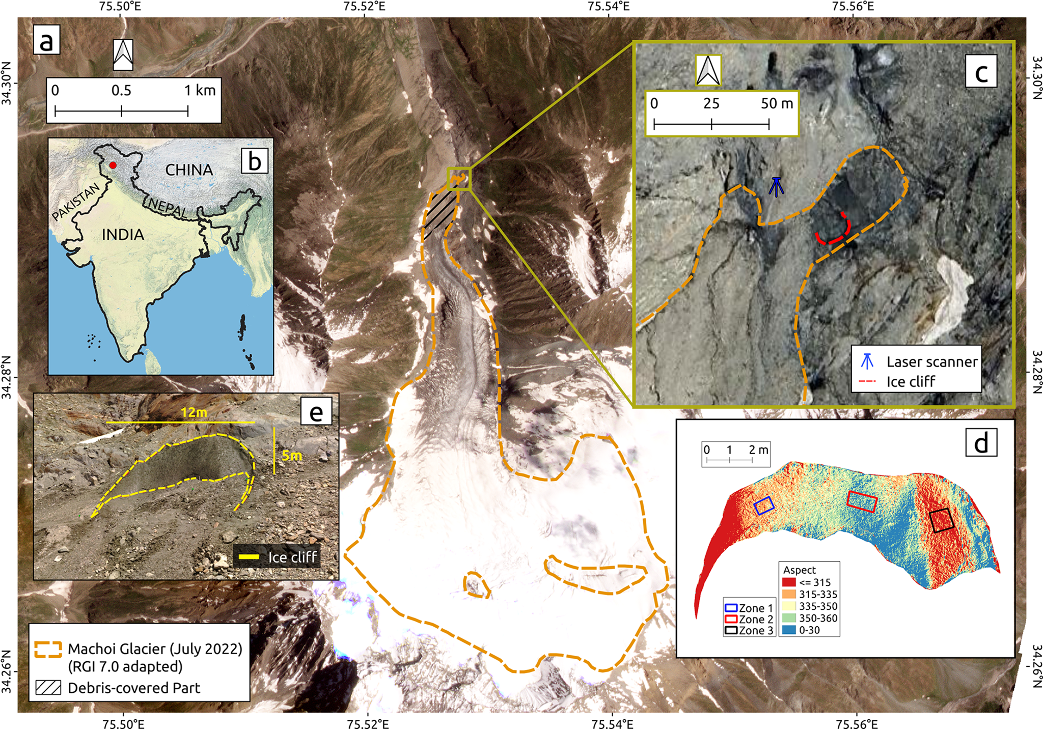
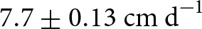
Figure 1. (a) Machoi Glacier, western Himalaya and its surrounding areas with the glacier boundary as of July 2022 (adapted from RGI 7.0; RGI Consortium 2023). Basemap source: Planet Labs, dated 29 June 2022. (b) An inset map shows the location of Machoi Glacier (red dot). (c) Glacier terminus area showing the ice cliff and the fixed TLS position on 29 June 2022 (image source: Google Maps, dated 7 July 2022). (d) An aspect map of the ice cliff displays three zones to analyse melting trends (see text for details). (e) Field photograph of the ice cliff.
This debris-covered part of the Machoi glacier exhibited several ice cliffs. We selected one of the prominent ice cliff approximately 50 m horizontal distance from the glacier terminus that was conveniently accessible during the field survey (Fig. 1c). Its dimensions were 12.5 m (length), 5 m (height) and 3 m (width) on 28 June 2022 (Fig. 1e). The ice cliff had a mean slope of ∼50∘, and its aspect ranged from 300∘ to 30∘ (facing northwest; Fig. 1d).
3. Data and methods
3.1. Terrestrial laser scanning data acquisition and processing
We employed a FAROⓈ Plus TLS, which operates at a wavelength of 1550 nm (near-infrared) and features a nominal range of observation from 0.6 to 350 m. The TLS maintains a narrow-ranging error of  $\pm 1\ \mathrm{mm}$, primarily as a systematic measurement error at distances between 10 and 25 m. Our survey period had favourable meteorological conditions devoid of fog, precipitation or strong winds, which could have compromised data quality due to interactions of the laser with atmospheric particles. The TLS was positioned on stable bedrock approximately 30 m from the ice cliff (Fig. 1c), and from there, the ice cliff was scanned seven times between 28 and 30 June 2022 (Table 1). We processed the raw point-cloud data using FARO Scene software to register the point cloud and eliminate non-essential movements (Le and Liscio, Reference Le and Liscio2019). We manually registered point cloud data acquired on different days by referencing seven to ten distinguishable stable off-glacier features (e.g., cracks and corners of rocks) (Fig. 2). Registration of intra-day scans on 29 June 2022 was not required as the TLS position was fixed. Afterwards, we applied the ‘Multi-Model to Model Cloud Comparison’ (M3C2) algorithm (Lague and others, Reference Lague, Brodu and Leroux2013) to quantify the distance between two point clouds (M3C2 difference product), corresponding to two different epochs along the local surface normal direction (Watson and others, Reference Watson, Quincey, Smith, Carrivick, Rowan and James2017b, Kneib and others, Reference Kneib2022). The M3C2 difference product (in metres) was then used to calculate horizontal melt (backwasting) and vertical melt (downwasting) by applying trigonometric transformations based on the slope of the ice cliff (Watson and others, Reference Watson, Quincey, Smith, Carrivick, Rowan and James2017b). Registration error was estimated by considering the differences in stable areas within a 50 m buffer zone around the TLS location. Ideally, the backwasting in stable areas should be zero. Therefore, we computed the median difference values from each pair of point cloud data over the stable area in the buffer zone (Hoaglin and others, Reference Hoaglin, Mosteller and Tukey1982, Höhle and Höhle, Reference Höhle and Höhle2009) and corrected the systematic bias by the corresponding median value. We also computed the Normalized Median Absolute Deviation (NMAD) and used it as the uncertainty in our estimates (Pieczonka and Bolch, Reference Pieczonka and Bolch2015, Vijay and Braun, Reference Vijay and Braun2016).
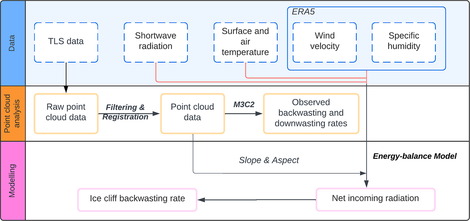
Figure 2. Workflow for ice cliff melt analysis. The top section shows the in-situ and climate reanalysis data used in the study. The middle section shows point cloud observation and processing. The bottom section shows the modelling of ice cliff backwasting rates, which uses slope and aspect derived from point cloud data.
Table 1. Date and time of scans for ice cliff observations
3.2. Energy-balance model
We simulated the hourly ice cliff backwasting rates over the study period using an energy-balance model (Sakai and others, Reference Sakai, Masayoshi and Fujita1998, Han and others, Reference Han, Wang, Wei and Liu2010). Here, we briefly outline the theory underlying the energy-balance model. All reasoning and mathematics behind the energy-balance model are provided in the supplementary material. The net heat flux  $ Q_\mathrm{m}$ available for ice cliff melting ( $\mathrm{W\ m}^{-2}$) is given by:
 \begin{equation}
Q_\mathrm{m} = I_\mathrm{n} + L_\mathrm{n} + H + LE
\end{equation}
\begin{equation}
Q_\mathrm{m} = I_\mathrm{n} + L_\mathrm{n} + H + LE
\end{equation} where  $ I_\mathrm{n}$, $ L_\mathrm{n}$, H and LE are the net shortwave radiation ( $\mathrm{W\ m}^{-2}$), net longwave radiation ( $\mathrm{W\ m}^{-2}$), sensible heat flux ( $\mathrm{W\ m}^{-2}$) and latent heat flux ( $\mathrm{W\ m}^{-2}$), respectively. To understand the role of solar position in the sky and associated radiation (shortwave) on ice cliff backwasting on an hourly scale, we used the method from Han and others Reference Han, Wang, Wei and Liu(2010), which states that the net shortwave radiation on an ice cliff slope in a unit-sloped area is
 \begin{equation}
I_\mathrm{n} = (I_\mathrm{s} + D_\mathrm{s} + D_\mathrm{t})(1 - \alpha)
\end{equation}
\begin{equation}
I_\mathrm{n} = (I_\mathrm{s} + D_\mathrm{s} + D_\mathrm{t})(1 - \alpha)
\end{equation} where  $ I_\mathrm{s}$, $ D_\mathrm{s}$, $ D_\mathrm{t}$ and α are direct solar irradiance from the sky ( $\mathrm{W\ m}^{-2}$), diffused sky irradiance ( $\mathrm{W\ m}^{-2}$), diffuse irradiance ( $\mathrm{W\ m}^{-2}$) from surrounding terrain and the albedo of the ice cliff, respectively. We used an Apogee pyranometer (Model: SP-510 & SP-610) for incoming global solar radiation measurements on 30 June 2022 (Table S1). Note that we did not measure global solar radiation on 29 June 2022, when we carried out hourly scale TLS measurements. We used the corresponding hourly global radiation values measured on 30 June 2022 to fill this data gap. This is reasonable as the atmospheric conditions during 28–30 June 2022 were similar (clear sky and no rain). Albedo measurements on the ice cliff were obtained using an SVC HR768i spectroradiometer. A mean albedo value of 0.07 was used in the model derived from two measurements recorded at 1430–1745 hours on 29 June 2022.
The net longwave radiation  $(L_\mathrm{n}$) comprises the incoming atmospheric longwave irradiance from the visible portions of the sky $(L_\mathrm{s}$), the incoming longwave irradiance from the surrounding terrain $(L_\mathrm{t}$) and the outgoing longwave irradiance $(L_\mathrm{o}$) (Eqn 3); all irradiances are in ( $\mathrm{W\ m}^{-2}$)
 \begin{equation}
L_\mathrm{n} = L_\mathrm{s} + L_\mathrm{t} - L_\mathrm{o}.
\end{equation}
\begin{equation}
L_\mathrm{n} = L_\mathrm{s} + L_\mathrm{t} - L_\mathrm{o}.
\end{equation} To calculate the longwave radiation component ( $L_\mathrm{s}$ and $L_\mathrm{t}$), we used the air (15 cm above the surface) temperatures ( $^{\circ}\mathrm{C}$), observed close to the ice cliff using a shielded Tomst TMS-4 temperature logger from 29 June 2022, 1330 hours to 30 June 2022, 0945 hours. For outgoing longwave radiation (and $L_\mathrm{o}$), the surface temperature of the ice cliff ( $^{\circ}\mathrm{C}$) assumed constant at $0^{\circ}\mathrm{C}$.
For the computation of the turbulent heat fluxes H and LE, vapour-pressure and wind-speed estimates were taken from the ERA5 reanalysis data (Copernicus Climate Change Service, Reference Muñoz2019), as no in-situ data were available. ERA5 data are available on an hourly scale at  $0.25^{\circ} \times 0.25^{\circ}$ grid resolution. The turbulent fluxes were calculated using the bulk aerodynamic formula given by Sakai and others Reference Sakai, Masayoshi and Fujita(1998). In the energy-balance model, we neglected the effect of conductive flux within the ice.
Given the value of  $Q_\mathrm{m}$, the melt rate (M) of the ice cliff ( $\mathrm{m\ s}^{-1}$) at any given epoch can be calculated as
 \begin{equation}
M = \frac{Q_\mathrm{m}}{\rho_{\text{ice}} L_\mathrm{f}},
\end{equation}
\begin{equation}
M = \frac{Q_\mathrm{m}}{\rho_{\text{ice}} L_\mathrm{f}},
\end{equation}  $ \rho_{\text{ice}}$ is the density of ice ( $900\ \mathrm{kg\ m}^{-3}$), $L_\mathrm{f}$ is the latent heat of fusion of ice ( $334\,\mathrm{KJ\ kg}^{-1}$), and then using the slope of the ice cliff, we estimated the backwasting rate from the melt rate. Equations (1) and (4) serve as the general formulas for deriving ice melt. Considering Buri and Pellicciotti Reference Buri and Pellicciotti(2018)’s illustration of how aspect influences the melting regime of ice cliffs, we considered adjusting the observed incoming global solar radiation based on the location of the ice cliff and the time of the TLS scan (Garnier and Ohmura, Reference Garnier and Ohmura1968). This adjustment allowed us to determine the sun’s position in the sky during each scan. Subsequently, we adjusted the amount of observed incoming global solar radiation received by the ice cliff by accounting for its slope and aspect (Fig. S1 and Eqns (S3–4)). These adjustments enable our analysis to reflect the effects of differential solar radiation exposure on the ice cliff, affecting its melting dynamics.
4. Results
4.1. Ice cliff backwasting
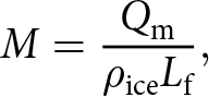
The mean ice cliff backwasting rate over the entire study period of 44 hours (1630 hours, 28 June to 1250 hours, 30 June) was  $0.26 \pm 0.003 \,\mathrm{cm\ h}^{-1}$. The mean backwasting rate during a 24-hour period between 1630 hours, 28 June, and 1630 hours, 29 June, was estimated to be $0.32 \pm{0.005} \,\mathrm{cm\ h}^{-1}$ (Table S2). However, the backwasting rates showed significant variations over shorter time scales. In particular, it varied from $0.38 \pm 0.05 \,\mathrm{cm\ h}^{-1}$ (1430–1530 hours) to $1.06 \pm {0.13} \,\mathrm{cm\ h}^{-1}$ (1530–1630 hours) on 29 June 2022 (Fig. 3). This ∼280% rise in hourly melt rates during the afternoon of 29 June 2022 coincided with the sun reaching the optimal solar elevation angle of ∼50∘ at 1530 hours. At this instant, the direct solar radiation available for melting at the studied ice cliff was maximum. Subsequently, the hourly rates steadily declined to $0.68 \pm 0.03\,\mathrm{cm\ h}^{-1}$ (1730–1830 hours) as the solar elevation angle changed to 13∘ (Fig. 3).
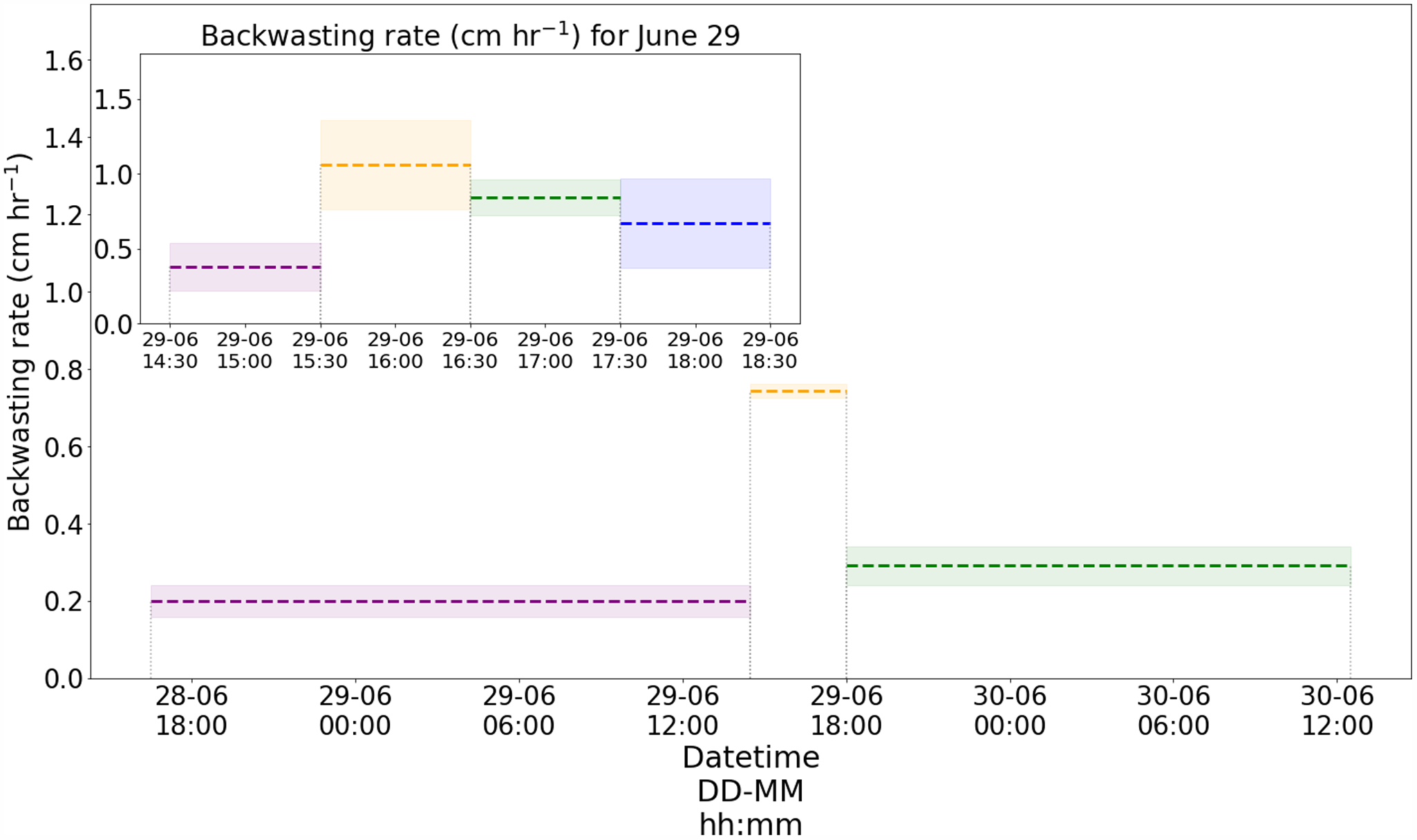
Figure 3. Dotted lines and vertically coloured spaces show the mean observed ice cliff backwasting rates and uncertainties between consecutive hourly and daily scans. The inset plot shows hourly backwasting rates ( $\mathrm{cm\ h}^{-1}$) observed on 29 June 2022.
4.2. Energy fluxes
During our hourly observations on 29 June 2022, the shortwave radiation over the ice cliff surface had majorly contributed to the ice cliff backwasting (Fig. 4a). Separating the net shortwave radiation into its components, direct solar radiation was the primary contributor to net shortwave radiation from 1430 to 1630 hours (Fig. 4b). It is worth noting that the maximum observed solar radiation by pyranometer ( $825\ \mathrm{W\ m}^{-2}$) occurs at the site during 1100 -1200 hours (Table S1). However, given the ice cliff’s slope and aspect, the aspect-corrected maximum net shortwave radiation of ∼680 $\mathrm{W\ m}^{-2}$ occurs between 1500 and 1700 hours. The shortwave radiation remained high during the late afternoon (after 1630 hours), with the diffused components being the main contributor until 1830 hours (Fig. 4b). From 1730 to 1830 hours, the aspect-corrected net shortwave radiation declined from ∼536 $\mathrm{W\ m}^{-2}$ to ∼250 $\mathrm{W\ m}^{-2}$.
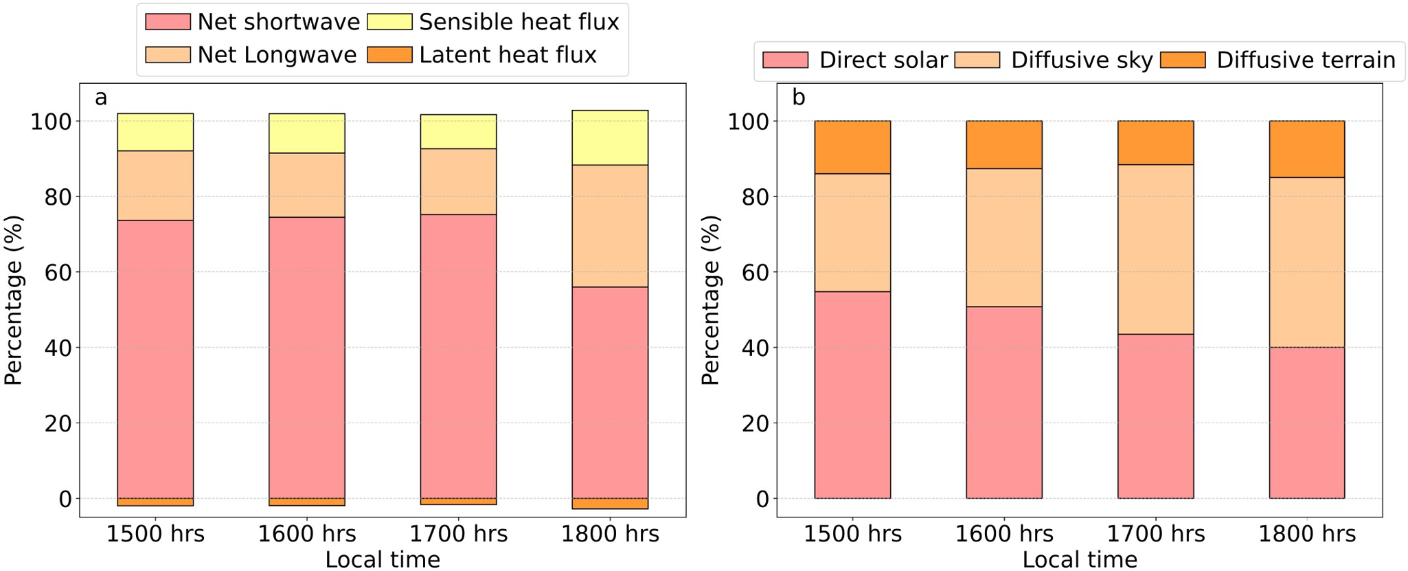
Figure 4. Partioning of (a) the total absorbed mean hourly radiative fluxes and (b) the available mean hourly net shortwave radiation at the ice cliff into the corresponding components during the late afternoon hours of 29 June 2022.
Temperature observations close to the ice cliff from 29 June 2022 to 30 June 2022 show that the air and surface temperatures above the debris were above  $0^{\circ}\mathrm{C}$ throughout the day and night. The minimum air and surface temperatures were $6^{\circ}\mathrm{C}$ and $3^{\circ}\mathrm{C}$, respectively, at around 0600–0700 hours (Fig. S2). The net longwave radiations, derived from surface and air temperatures, remained relatively stable (140–160 $\mathrm{W\ m}^{-2}$) on an hourly scale during 1430–1830 hours on 29 June 2022.
4.3. Spatial and temporal variability of ice cliff backwasting
In addition to offering high temporal resolution estimates of the ice cliff’s mean backwasting rates, the TLS data also provide a detailed view of the backwasting pattern within the cliff at a very high spatial resolution with an average spacing of 2–3 mm (Fig. 5). The observed hourly backwasting pattern rate has a large spatial variability of up to 65% relative to the corresponding mean value. This spatial variation and pattern shifts systematically with the sun’s position. Beyond the visual pattern of the backwasting, we also compared the modelled and observed backwasting rates in three different representative zones within the ice cliff (Table S3). For zone 1 and zone 2, the modelled and observed values match reasonably well without any additional fine-tuning or calibration of the model parameters. However, the values were not in agreement in zone 3.
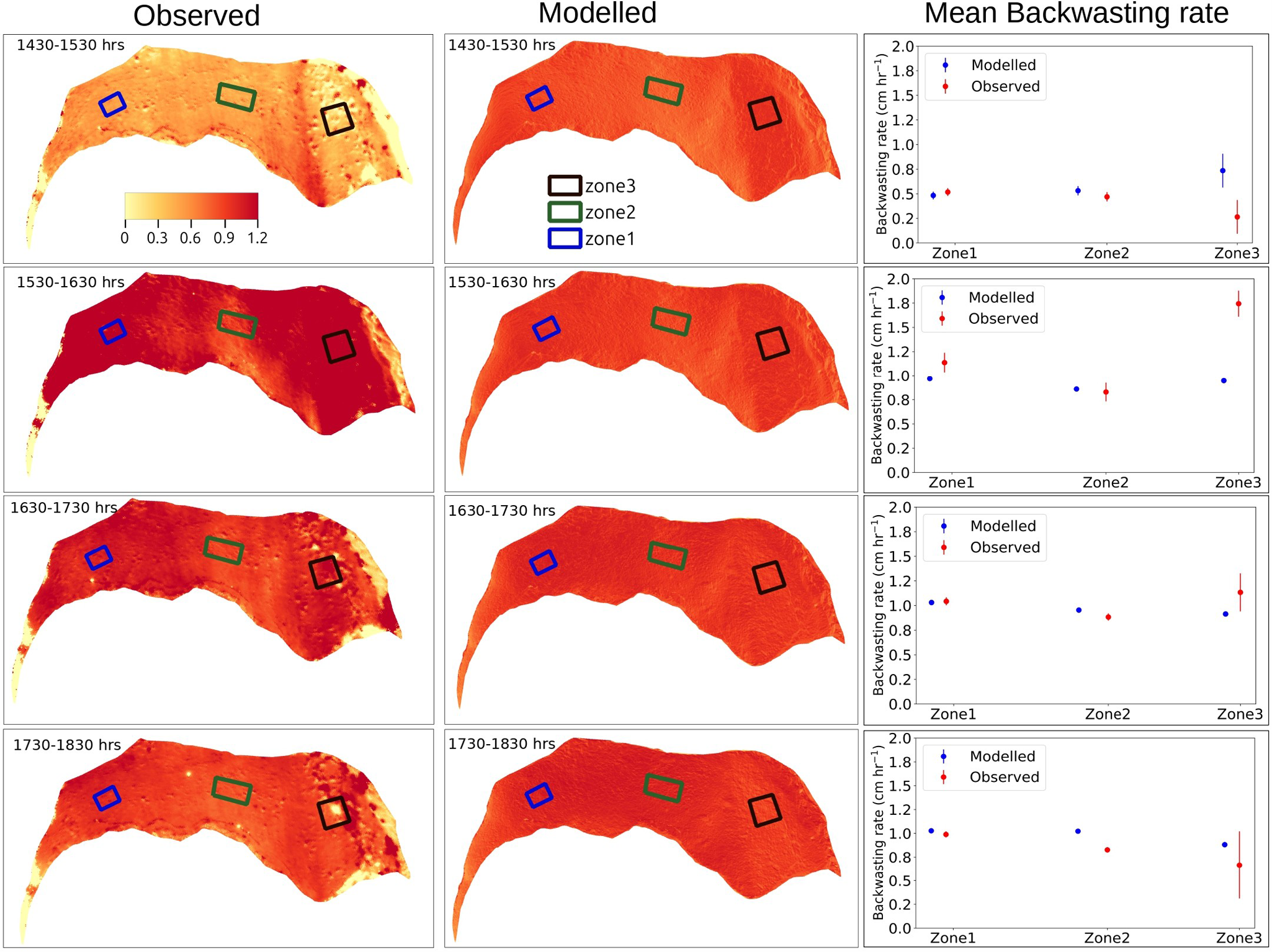
Figure 5. Comparison between observed (left column) and modelled (middle column) ice cliff backwasting rates, with colour scale representing the rates in  $\mathrm{cm\ h}^{-1}$. The right column presents the plots showing the mean observed and modelled backwasting rates of three zones.
5. Discussions
5.1. Feasibility of TLS for ice cliff monitoring
Theoretically, the 1550 nm wavelength TLS used in this study is not ideal for ice monitoring due to the low reflectance of snow and ice (Deems and others, Reference Deems, Painter and Finnegan2013). However, debris-covered regions can be effectively monitored using such a TLS. In this study, the ice cliff was covered by a layer of fine debris (Fig. 1e), which enabled a substantial amount of reflected beam and allowed for precise monitoring of ice cliff changes using such a TLS in similar environments despite theoretical limitations.
Similar studies on ice cliffs have used GNSS data to coregister the TLS point clouds. However, coregistration using GNSS does not necessarily improve the accuracy and can often increase co-registration errors (Brun and others, Reference Brun2016, Reference Brun2018, Watson and others, Reference Watson, Quincey, Smith, Carrivick, Rowan and James2017b). In this study, we could not coregister the point clouds using GNSS observations due to the failure of the GNSS device. Our assessment of errors after coregistration using prominent features demonstrates TLS feasibility in ice cliff monitoring on a diurnal scale, allowing for detecting changes at the millimetre scale. This enabled us to use TLS data to monitor the hourly backwasting rate, which was not possible with other geodetic methods used in previous studies. The observed mean hourly backwasting rates reached up to  $0.74\ \mathrm{cm\ h}^{-1}$, more than twice as large as our presented mean daily estimates. This hourly value is also significantly higher than the published sub-seasonal/seasonal-scale estimates (Table 2), indicating how the hourly variations can be better resolved using the TLS.
Table 2. Backwasting rates (with uncertainties in cm) for ice cliffs from different studies using various methods

5.2. Influence of radiation and topography on ice cliff backwasting
Relatively high net radiation during the late afternoon is primarily due to the contributions of the diffused shortwave components and the net longwave radiation. This diurnal variation in radiation closely aligns with observed backwasting rates, which are the highest (1500–1700 hours) during periods of maximum solar radiation on the ice cliff. The high radiation in the late afternoon coincides with a relatively high melt rate, emphasizing the role of both direct and diffused radiations in ice cliff backwasting. Thus, the relatively large differences between mean hourly and mean daily backwasting rates discussed in the previous section are largely due to the strong diurnal variability of net radiation (Reid and Brock, Reference Reid and Brock2014).
The ice cliff backwasting spatial variation is majorly controlled by the local aspect, and as a result, the pattern shifts systematically with the sun’s position. This interpretation is supported by the corresponding model results, which largely align with the observations (Fig. 5). However, the observed and modelled values were inconsistent in zone 3 (Table S3). This discrepancy may stem from the larger variation in aspect observed in zone 3 ( $310^{\circ} \pm 14^{\circ}$) compared to zone 1 ( $328^{\circ} \pm 7^{\circ}$) and zone 2 ( $0^{\circ} \pm 8^{\circ}$). Additionally, we relied on point-based temperature and wind velocity observations to calculate longwave radiation and heat fluxes in the energy-balance model. These fluxes are key contributors to backwasting rates and patterns; however, point-based data may overlook subtle variations, introducing certain uncertainties. Additionally, we did not account for conductive flux within the ice, which further limits the model’s accuracy. As a result, we cannot expect an ideal match between modelled and observed values.
5.3. Comparison with other studies
In the Himalaya, previous studies have reported ice cliff backwasting rates at different temporal resolutions: weekly (Kneib and others, Reference Kneib2022), monthly (Han and others, Reference Han, Wang, Wei and Liu2010) and seasonally (Sakai and others, Reference Sakai, Masayoshi and Fujita1998, Brun and others, Reference Brun2018). Based on these studies, the backwasting rates generally vary from 0.7 to  $11\ \mathrm{cm\ d}^{-1}$ (Table 2). The daily scale value observed in our study is $7.7 \pm {0.13}\ \mathrm{cm\ d}^{-1}$, which is within the range of previously reported rates (Table 2). Notably, the backwasting rates on a daily scale are comparable across these studies despite different terrestrial data collection methods, including ablation stakes (Sakai and others, Reference Sakai, Masayoshi and Fujita1998, Han and others, Reference Han, Wang, Wei and Liu2010, Steiner and others, Reference Steiner, Buri, Miles, Ragettli and Pellicciotti2019), terrestrial photogrammetry (Brun and others, Reference Brun2016, Watson and others, Reference Watson, Quincey, Smith, Carrivick, Rowan and James2017b, Kneib and others, Reference Kneib2022) and TLS (present study). However, the uncertainties reported in the previous studies are at the order of magnitude or larger than the TLS-based method employed in this study. Our hourly scale observations show that shortwave radiation remains the dominant contributor to net radiation. Meanwhile, studies observing ice cliffs over extended periods (monsoon, pre-monsoon and post-monsoon phases) reveal that varying weather conditions affect the contributions of different radiation fluxes to net radiation. For example, during monsoon periods, increased cloud cover often reduces direct shortwave radiation (Steiner and Pellicciotti, Reference Steiner and Pellicciotti2016), while longwave flux may become a more significant contributor than total shortwave flux (Buri and others, Reference Buri, Miles, Steiner, Immerzeel, Wagnon and Pellicciotti2016a).
5.4. Implications of ice cliff backwasting on glacier scale
Satellite-based studies reported  $0.95\ \mathrm{cm\ d}^{-1}$ ( $3.5\ \mathrm{m\ yr}^{-1}$) during 2000–2016 (Brun and others, Reference Brun, Berthier, Wagnon, Kääb and Treichler2017) and $0.8 \ \mathrm{cm\ d}^{-1}$ ( $3.1\ \mathrm{m\ yr}^{-1}$) during 2015–2020 (Hugonnet and others, Reference Hugonnet2021) of thinning rates for the debris-covered part of Machoi Glacier (Fig. 1a). Here, we used published thinning rate datasets over debris-cover parts from Brun and others Reference Brun, Berthier, Wagnon, Kääb and Treichler(2017) and Hugonnet and others Reference Hugonnet(2021) and scaled them down to daily rates. The ice cliff downwasting (thinning rate), as derived from our observed ice cliff backwasting rate, is at the order of $7.7 \pm {0.13} \ \mathrm{cm\ d}^{-1}$ on a daily scale (considering the ice cliff’s median slope of 45∘). Considering this rate, the studied ice cliff would have lost about 5 m of height over the next 2 months. This explains why it vanished completely by our second expedition to the glacier on 4–8 September 2022 (Fig. S3). Considering that the debris-covered part of Machoi Glacier (∼9.1 ×10⁴ m2) continued thinning at an average rate of $0.8 \ \mathrm{cm\ d}^{-1}$ (Hugonnet and others, Reference Hugonnet2021) in 2022, and applying interpolation and scaling of our ice cliff downwasting rate, we estimate that our investigated ice cliff accounted for 0.4% of the total thinning in the debris-covered part in 2022. Brun and others Reference Brun(2018) showed that 144 ice cliffs (∼8% of total tongue area) of different sizes contributed 23% of the ablation of the debris-covered part of Changri Nup, Nepalese Himalaya. Similarly, 11.7% ice cliff coverage in the debris-covered tongue was found to contribute 26% to the total melting of the debris-covered tongue in the Kennicott Glacier, Alaska, USA (Anderson and others, Reference Anderson, Armstrong, Anderson and Buri2021a). We noticed many melting ice cliffs at Machoi Glacier during the fieldwork, although not recorded in this study. If we consider a hypothetical scenario where several ice cliffs of total area ∼2200 $\mathrm{m}^{2}$ (∼2% of the debris-covered part) on Machoi Glacier melted at the same rate during the ablation period of 2022 (Fig. S4), they could have potentially augmented the thinning rate of the debris-covered area by 17.5%. Due to the ice cliffs formation, persistence, and decay on debris-covered areas over time (Brun and others, Reference Brun2018, Steiner and others, Reference Steiner, Buri, Miles, Ragettli and Pellicciotti2019, Sato and others, Reference Sato2021), we expect that these ice cliffs can significantly influence local glacier surface energy and mass balance processes in debris-covered part (Moore, Reference Moore2018, Buri and others, Reference Buri, Miles, Steiner, Ragettli and Pellicciotti2021, Kneib and others, Reference Kneib2021, Reference Kneib2023).
6. Conclusions
We estimated hourly to daily scale backwasting rates of an supraglacial ice cliff on Machoi Glacier, western Himalaya, by differencing multi-temporal 3D point-cloud data captured using a TLS. Our study revealed that despite theoretical limitations, our 1550 nm wavelength TLS could precisely map the ice cliff topography due to highly reflecting fine debris covering the ice cliff. The uncertainties were mainly due to point cloud co-registration and were on the order of millimeters level, which is suitable for estimating daily backwasting rates. We observed significant temporal variability in backwasting rates, reaching up to approximately threefold rise from  $0.38\;{\mathrm{cm}\;\mathrm h}^{-1}$ between 1430 and 1530 hours to $1.06\,\mathrm{cm\ h}^{-1}$ between 1530 and 1630 hours. Our observed daily backwasting rates are consistent with previous studies in the Himalaya, while the peak hourly scale backwasting rate is substantially higher than previously reported daily or seasonal averages. Our energy-balance modelling revealed that this short-time variability was primarily driven by direct solar radiation, given the slope and aspect of the cliff. As the day progress, net longwave radiation becomes increasingly significant. These findings highlight that the geometry of ice cliffs and variations in solar position are critical drivers of the short-term variability in complex microscale melt patterns. A good agreement between the observed backwasting rates and those predicted by the energy-balance model ascertained the ability of the model to capture the essential dynamics of ice cliff melting even at an hourly scale. This implies that high-resolution temporal and spatial monitoring of ice cliffs with TLS over a relatively short period can inform and improve the large-scale mass-balance models of debris-covered glaciers. Additionally, it is crucial to include in situ meteorological data to force the energy-balance model, as this ensures that the simulations accurately reflect local conditions and match the observed data.
Supplementary material
The supplementary material for this article can be found at https://doi.org/10.1017/jog.2024.98.
Acknowledgements
The authors extend their gratitude to the Prof. Hester Jiskoot (Associate Chief Editor), Fanny Brun (Scientific Editor), Lynsey Rowland (Editorial Assistant) and the two anonymous reviewers for their insightful comments and suggestions, which significantly improved the manuscript. We also express our gratitude to Nadeem Ahmad Najar, Imtiyaz Ahmad Bhat, Faisal Zahoor Jan and Danish Kashani from the University of Kashmir, Amit Singh Chandel from IIT Madras and Manzoor Ji from Matayen village for their invaluable support in the field.
Author contributions
PS and SV conducted the TLS data acquisition, analysed the data and wrote the manuscript. PS, SV, AB and CS contributed to the energy-balance modelling and manuscript-related discussions. IR assisted in collecting all data and contributed to the discussions. SAZ assisted in processing radiation observation data. All authors have reviewed and approved the final version of the paper for publication.
Financial support
This research has been supported by the Faculty initiation grant (grant no. FIG-100918) by sponsored research and industry consultancy Indian Institute of Technology Roorkee and a scholarship from the Ministry of Education (MoE), India. Open Access funding is granted by Indian Institute of Technology Roorkee.


 Open access