


1. Introduction
The Greenland Ice Sheet (GrIS) expresses high variability in ice loss, and hence sea level rise, due to the regional scale variability in the processes governing mass balance (Lenaerts and others, Reference Lenaerts, Medley, van den Broeke and Wouters2019). Surface mass balance (SMB) contributes just over half ($\sim \!52 \%$ ) of GrIS mass loss, but ice-sheet wide SMB simulated from regional climate models maintains $\sim \!25 \%$
 uncertainty (Shepherd and others, Reference Shepherd2020). Efforts to improve SMB simulation (e.g. Fettweis and others, Reference Fettweis2017) are limited by the scarcity of observations, which are required to evaluate the model performance (e.g Noël and others, Reference Noël2016). Traditionally, SMB measurements are made at the point scale during infrequent field efforts, through the laborious process of excavating snow pits or drilling firn cores. The sparseness of snow pit observations on the GrIS limits the testable correlation lengths and tends to debilitate spatial correlation analysis. Consequentially, surface density measurements have shown no spatial correlation over length scales of tens to hundreds of kilometers (Fausto and others, Reference Fausto2018). Due to the unknown variability of density and SMB, point measurements used to parameterize a firn model (e.g. Zwally and Li, Reference Zwally and Li2002) must be extrapolated to regional scales cautiously. In space-borne altimetry retrievals of GrIS mass balance, the uncertainty in modeled corrections for snow densification required to convert a measured change in ice-sheet volume to a change in mass causes $\sim \!16 \%$
 uncertainty (Shepherd and others, Reference Shepherd2020).
Ground-penetrating radar (GPR) surveys are capable of imaging layers of accumulated snow (e.g. Vaughan and others, Reference Vaughan, Corr, Doake and Waddington1999). However, conventional, single-offset GPR analysis requires an independent measurement of firn density to estimate the accumulation (Navarro and Eisen, Reference Navarro, Eisen, Pellikka and Rees2009). Point SMB measurements often provide the required density information to extrapolate the density profile along the track of the radar sounding (e.g. Hawley and others, Reference Hawley2014; Overly and others, Reference Overly, Hawley, Helm, Morris and Chaudhary2016). Yet, relying on sparse firn cores to extrapolate density over tens to hundreds of kilometers may bias the derived accumulation estimates. For example, ice lenses sampled in a firn core increase the average density and can be incorrectly extrapolated over tens of kilometers, as these features are uncorrelated over tens of meters (Brown and others, Reference Brown, Harper, Pfeffer, Humphrey and Bradford2011). For the period 1971–2016, greater than $10 \%$ bias to the SMB is possible, when firn cores are not available for extrapolation (Lewis and others, Reference Lewis2019). Inaccuracies are greater in southern Greenland, which is experiencing increasing near-surface firn densification as a result of atmospheric warming (Graeter and others, Reference Graeter2018), than in central Greenland. Parameterization of snow and firn densification continues to improve (e.g. Meyer and others, Reference Meyer, Keegan, Baker and Hawley2020); yet, evolving the firn using full energy balance modeling remains operationally challenging and is limited spatially by the unknown heterogeneities of surface snow density, accumulation and melt (Vandecrux and others, Reference Vandecrux2018). Surface snow density parameterizations formulated around temperature and wind speed (e.g van Kampenhout and others, Reference van Kampenhout2017) are arguably less preferable than density measurements because of uncertainties in estimating wind speed and modeling the unknown length scale variability that exists in the GrIS snow (Fausto and others, Reference Fausto2018).
Radar retrievals of snow density are an appealing alternative to in situ observations of snow and firn because the methods are non-destructive and rapidly acquire vast amounts of data. However, few methods for continuously mapping snow and firn density exist (e.g. Grima and others, Reference Grima, Blankenship, Young and Schroeder2014) due to the complexities of data inversion. In this work, we present the analysis of multi-channel, multi-offset, radar (MxRadar) imagery along a 78 km traverse in the GrIS dry snow accumulation zone to demonstrate the capability of this method, which has the advantage of ascertaining snow and firn density, and depth, and thereby SMB, independently. Of the previous studies applying GPR velocity analysis, none have performed continuous estimates throughout tens of kilometers distance (e.g. Bradford and others, Reference Bradford, Nichols, Mikesell and Harper2009). We based our MxRadar workflow on the analysis of the radar surface wave, which exhibits linear moveout (LMO), and the fall 2014 isochronous reflection horizon (IRH) to estimate the surface snow density, column average density, horizon depth and 2015–2017 SMB. We then input our data into the Herron and Langway (Reference Herron and Langway1980) firn density and age model. We use the firn model to further enhance the MxRadar imagery and extend the historical period of the SMB reconstruction to 1984–2017 with instantaneous (~14 days) temporal intervals. We compare the resulting SMB against a firn core and quantify the length of spatial correlation that exists in surface snow density. We quantify the bias reduction in SMB derived using the measured-modeled, MxRadar–Herron and Langway (Reference Herron and Langway1980) method. Then we provide a discussion of the results, limitations and advantages of the method, and future directions. We developed our analysis within the interior region of Greenland where there was significant spatial variation in accumulation, but little melt, to develop confidence in this type of radar retrieval for density and SMB.
2. Greenland Traverse for Accumulation and Climate Studies
The Greenland Traverse for Accumulation and Climate Studies (GreenTrACS) is a multi-disciplinary study of recent SMB changes in the West Central percolation and dry snow accumulation zones of the GrIS. During the Spring of 2016 and 2017, we traveled a total of 4436 km by snowmobile from Raven/DYE-2 to Summit Station along the elevation contour straddling the percolation zone, and along West-East ‘spurs’ perpendicular to the elevation contours. Throughout the expedition, we collected 16 shallow (22–32 m) firn cores and dug 42 snow pits; 16 pits were coincident with the cores and the 26 others were dug at the ends of the spurs (Figs 1 and 2). Our GreenTrACS field seasons occurred prior to the on-set of melt to reduce the complexity of radar data inversion. The cores and the coincident snow pits were sampled for density, isotopic chemistry, dust and trace elements to define annual layer depths for measuring SMB (e.g. Graeter and others, Reference Graeter2018; Lewis and others, Reference Lewis2019). As firn cores are strategically located point measurements, GPR imagery is often leveraged to spatially extend the record of firn stratigraphy between core sites for accumulation studies (e.g. Spikes and others, Reference Spikes, Hamilton, Arcone, Kaspari and Mayewski2004; Miège and others, Reference Miège2013). We operated a suite of radar instruments spanning the frequency range 0.4–18 GHz; the focus of this study is the MxRadar.
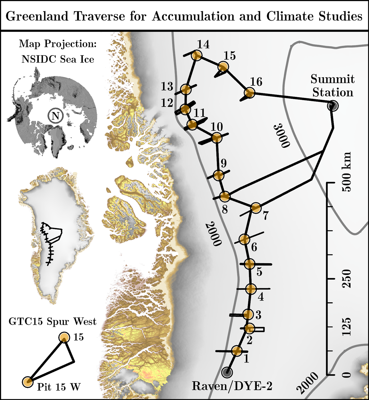
Fig. 1. GreenTrACS firn cores (GTCs) are numbered 1–16. Ground-penetrating radar surveys were conducted along spur traverses and the main route that links the GTCs. We developed our radar processing and analyses at GTC15 Spur West (lower left inset). The 2000 m asl contour envelopes the western spurs. Surface elevation was acquired from Morlighem (Reference Morlighem2017) and Porter and others (Reference Porter2018).

Fig. 2. Topographic profile of GreenTrACS Core 15 Spur West. The topographic undulation near Pit 15 W is responsible for increases and decreases in accumulation. The initial 15 km, up to the point of maximum elevation of the profile, are directed into the predominant wind, making this a leeward slope. The predominant wind blows approximately orthogonal across the next 30 km of the GTC15 Spur west traverse and is 21.5° oblique to the final 33 km of GTC15 Spur West.
2.1. Study area
GreenTrACS Core 15 (GTC15) is the second most northern core site of the GreenTrACS campaign (47.197°W, 73.593°N) and is ~2600 m above sea level. GTC15 had an average annual temperature of −25.7 ± 1.0°C (Modern-Era Retrospective analysis for Research and Applications (MERRA), 1979–2012), and an average annual SMB of 0.306 ± 0.021 m w.e. a−1 (1969–2016). The site experiences little to no melt, measured as the average melt feature percentage determined by normalizing each year's ice layer water equivalent by the annual water equivalent and then averaging ($0.47 \%$ , 1969–2016).
GTC15 Spur West is a triangular, clockwise circuit that departs from and returns to GTC15 (Fig. 1 inset). The first of three transects is 15 km in length, bearing 157°, and begins at GTC15. The second transect is 30 km in length at 246.5° which ends at Pit 15 W. The final transect is 33 km in length from Pit 15 W to GTC15 and bearing 40.5°. The GrIS surface of GTC15 Spur West was wind-affected snow with sastrugi $\lessapprox 25\, {\rm cm}$ in height. We estimated the average meteorological wind direction of 152° using monthly 10 m zonal and meridional wind speeds from the ensemble of the third generation reanalysis models (GEN3ENS) for the period 1979–2012 (Birkel, Reference Birkel2018). The average wind direction is approximately parallel to the first transect of GTC15 Spur West, approximately orthogonal to the second transect, and 21.5° oblique to the third transect. The cyclicity in the topographic profile (Fig. 2) results from our return to GTC15 along a path oblique to the path approaching Pit 15 W. The SMB changes significantly across the $\lessapprox 5\, {\rm km}$
 wide trough between distances 40–50 km. But, we do not observe preferential windward and leeward affects to the accumulation pattern here, because the orientation of the transects crossing this topographic trough are approximately orthogonal to the average wind direction. We selected this particular spur to develop our processing and analyses because of the apparent interplay between the surface elevation, SMB and heterogeneous layering observed in the radar imagery. Yet, we have foregone any topographic corrections in the radar processing.
2.2. Field methods
The MxRadar is a Sensors & Software 500 MHz GPR deployed with a multi-channel adapter in a multi-offset configuration using three transmitting and three receiving antennas (Fig. 3). During data acquisition, the transmitting and receiving channels were multiplexed to form nine radargrams which have independent antenna separations (offsets). The antennas were co-polarized, perpendicular to the direction of travel, and all are specified at 500 MHz with greater than two octave bandwidth. However, dependent on the antenna pairing, the actual central frequency and bandwidth varied on the order of tens of MHz. Our methods and analysis are tailored to produce meaningful data for the evaluation and improvement of snow cover and firn models and regional climate and reanalysis modeling of SMB.

Fig. 3. The MxRadar streamer array has three transmitting (Tx) and three receiving (Rx) antennas, which form nine independent offsets that were linearly spaced from 1.33 to 12 m apart. We simultaneously acquired nine continuous radargrams (one for each constant offset) and then binned the source-receiver pairs into common-midpoint (CMP) gathers.
3. Analysis methods
We review multi-offset GPR methods for SMB calculations in Section 3.1 to clarify the advantages of the multi-offset technique that are also important for interpreting the results. We provide much of the methodological detail in the Supplementary Material S.1. Here, we touch on the methodology to simplify our strategy for reconstructing the historical SMB for the period 1984–2017 along GTC15 Spur West. We considered SMB rather than the accumulation rate because of unaccounted mass lost to sublimation and ablation. SMB is conventionally measured using GPR by interpreting a select few IRHs using a constant age interval and applying the average normalized firn density over this interval (e.g. Lewis and others, Reference Lewis2019). Instead, we relied on the models of density and age, which were discretized in depth at a comparable resolution to the GPR data, and generated a SMB model with instantaneous (~14 day) temporal intervals (Section S.1.3). We averaged annual SMB from many realizations of the instantaneous SMB model in a Monte Carlo simulation to assess uncertainty (Section S.1.4). We estimated the multidecadal average SMB, invoking the central limit theorem, by repeatedly drawing from 10 of the 33 annual SMB distributions at random and averaging.
To parameterize the firn model, we first completed conventional signal processing on the nine radargrams, which consisted of a two octave bandpass filter around 500 MHz, amplitude gain corrections for wavefront spreading, coherent noise removal (background subtraction) and random noise removal (smoothing). Then we interpreted the air wave, surface wave and a shallow reflection (Fig. 4) on each of the nine images using a semi-automatic picking algorithm (Section S.1.1). We inverted the travel-times of the surface wave and the shallow reflection (see Section 3.1.1) to estimate the average electromagnetic (EM) propagation velocity and depth of the dry snow and firn in a least-squares approach (Section S.1.2), which used random resampling of the data to estimate uncertainties (Section S.1.4). We then applied a petrophysical model (Wharton and others, Reference Wharton, Hazen, Rau and Best1980) which relates the EM velocity of dry snow and firn to its density (Section S.1.3).
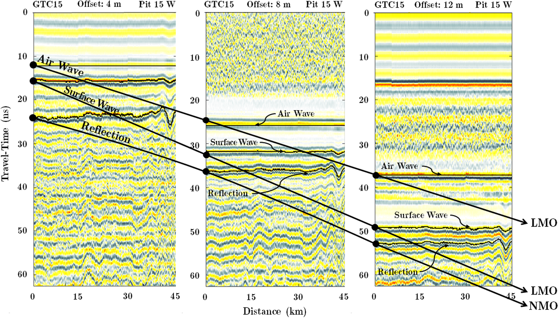
Fig. 4. This offset gather is represented by radargrams recorded at offsets 4, 8 and 12 m along the initial 45 km of GTC15 Spur West, and is annotated to convey the waveforms used in our analysis and the concepts of normal moveout (NMO) and linear moveout (LMO). Consider the traces at zero distance for each offset as a CMP gather. The air wave and surface wave arrivals are modeled by a linear expression of travel-time as a function of offset (Eqn (S.1)). The air wave is the first to arrive and expresses a more shallow slope (faster velocity) than the surface wave which is impeded while traveling through the snow. The annotated reflection expresses non-linear moveout which is approximated by NMO (Eqn (S.2)). The surface-wave (LMO) and reflection (NMO) annotated in this diagram are used to estimate the surface snow density, average snow density and depth of the fall 2014 isochronous reflection horizon (IRH). The age of the horizon was determined at GTC15 and allowed us to estimate the 2015–2017 SMB (see Supplement S.1.3), and in turn, is used to parameterize the HL model (see Supplement S.1.5).
Our measured-model approach relied on the Herron and Langway (Reference Herron and Langway1980) empirical firn density and age model, hereafter HL, which requires three input parameters: average snow density, average annual accumulation and 10 m firn temperature. We parameterized the HL model with the MxRadar snow density, MxRadar SMB (2015–2017) and MERRA 2 m air temperature as a proxy for firn temperature (Loewe, Reference Loewe1970), to model the stratigraphic age and density of the firn. We assessed the firn model accuracy and sensitivity to parameterization to illustrate the accuracy of the MxRadar-HL (MxHL) firn density (Section S.1.5). We justified tuning the age model to improve our estimates of SMB in a process that jointly updated the age-depth and SMB models according to the radiostratigraphy. The age model allowed us to convert the time domain radar image into the stratigraphic age domain, known as the Wheeler (Reference Wheeler1958) domain. In principle, the firn structure can be estimated by the age model because the stratigraphy was deposited in isochronous layers. The imaged firn structure can be flattened by converting the time domain GPR image into the Wheeler domain because the rows of the Wheeler image maintain a constant age. We ensured the relative structure of the age model by picking five horizons of the Wheeler transformed radiostratigraphy with an average epoch of 5.3 ± 2.7 years (the latest being the 1991 horizon) and perturbing the age model with the interpolated residuals to re-flatten the Wheeler image. We developed a structure-oriented noise-suppression filter which operates along the radar reflection horizons in the Wheeler domain to eliminate remnant noise after conventional GPR signal processing (Section S.1.6). This innovative signal processing technique allowed SMB estimates to depths at which previously the stratigraphy was uninterpretable due to the low signal-to-noise ratio. We then converted the filtered radargram from the Wheeler domain into the depth domain and interpreted 16 IRHs with an average epoch of 2.1 ± 1.7 years dating back to 1984. We calculated the error between the GTC15 geochemically determined age-depth scale and the 16 picked IRHs and interpolated a second grid of perturbations which we applied as a final update to the age model. We calculated the instantaneous SMB by taking a numerical derivative of the age-depth model (dz/da) and multiplying it by the MxHL density model (Eqn (S.20)).
3.1. Review of multi-offset radar
Common-midpoint (CMP) radar surveys are practiced in glaciology to estimate the EM wave speed of the ice, air and/or water mixture (e.g. Eisen and others, Reference Eisen, Nixdorf, Wilhelms and Miller2002). The wave speed is related to firn density and liquid water content using a dielectric mixture formula for a two or three phase relationship (e.g. Looyenga, Reference Looyenga1965; Wharton and others, Reference Wharton, Hazen, Rau and Best1980). In most studies, the CMP survey is treated as a point measurement of the firn vertical density profile, which is less laborious than extracting a core, but offers less vertical resolution and accuracy. Prior to GreenTrACS, CMP experiments on ice sheets were limited to point observations. We synthesized continuous CMP data by towing a streamer of nine antenna pairs that were linearly spaced from 1.33 to 12 m apart (Fig. 3). While the antenna pairs in this deployment did not have a common midpoint, we rebinned the constant offset radargrams for each pair independently, such that the analysis was performed on offset gathers with common midpoints.
3.1.1. Interpreting the near-surface waves
Numerous geophysical methods exist for velocity analyses of CMP data gathers. Analyses of reflection data can be divided into two fundamental categories by the question, ‘Does the analysis assume normal moveout?’ Normal moveout (NMO) is the reflection travel-time dependence on offset that arises from a homogeneously-layered and planar subsurface structure (within the distance of the maximum antenna offset) that exhibits small vertical velocity heterogeneity (Al-Chalabi, Reference Al-Chalabi1974). Previous studies avoided classical NMO analysis, instead using less automated, more computationally expensive methods that favored accuracy (Bradford and others, Reference Bradford, Nichols, Mikesell and Harper2009; Brown and others, Reference Brown2012, Reference Brown, Harper and Humphrey2017). Many caveats of NMO velocity analysis and sources of error in the radar common-midpoint analysis are discussed in Barrett and others (Reference Barrett, Murray and Clark2007). We demonstrate that NMO analysis of the snow and shallow firn yields a satisfactory result for data with low noise (see Supplement S.1.5), as ice-sheet stratigraphy in the high elevation accumulation zone is close to homogeneous and planar at the length scale of the radar streamer array.
Linear moveout (LMO) is the one-way travel-time dependence on offset of radar waves traveling directly from the transmitter through the air over the ice sheet and through the snow under the ice-sheet surface to the receiver antenna. We assumed that the air wave expresses the linear moveout velocity c ≈ 0.2998 m/ns to calibrate the timing of the multi-channel system (Section S.1.2). To analyze the surface wave, we assumed that the shallow, surficial snow is also planar and homogeneous at the scale of the maximum offset. We identified the air wave, surface wave and a near surface reflection and their respective moveout behavior in Figure 4. The travel-times of these waves were interpreted using a horizon tracking algorithm (see Supplement S.1.1). The linear methods for LMO and NMO velocity analysis are described in Section S.1.2 and the methods for estimating the surficial and average snow density and depth of the fall 2014 IRH are discussed in Section S.1.3. We quantified the uncertainty of the density, depth, age and SMB used to parameterize the HL model in Section S.1.4.
3.1.2. Critically refracted waves
Lateral energy travels on direct raypaths from transmitter to receiver, but also on raypaths that are critically refracted at the free-surface. An upgoing reflected wave can become critically refracted along the air/snow interface upon exiting the snow surface. These refracted waves appear in Figure 4 as multiple air wave arrivals succeeding the initial air wave. In Section S.1.2.1, we provide a discussion of the critically refracted wave phenomena with an accompanying snowpack model and exercise to support and demonstrate the critically refracted raypath.
3.2. Spatial correlation of surface snow density
The LMO and NMO estimated snow densities are independent measurements of the snow density above the interpreted radar horizon. The GPR surface wave maintains a fairly consistent depth level (~0.5 m, Eqn (S.17)), but the NMO reflection horizon does not. To mitigate the effects of depth on the correlation, we extracted the rows of the MxHL density model corresponding to the average depth of the LMO (0.5 m) and NMO (1.92 m) horizons interpreted for velocity analysis (Fig. 4). We used Pearson (Reference Pearson1907) correlation to determine the relationship between the density at 0.5 m depth and the density at 1.92 m depth. Additionally, we conducted variogram analysis (Matheron, Reference Matheron1963) on the LMO estimated snow density for each of the three transects of GTC15 Spur West. We determined the length scale over which there is consistent spatial correlation of the surface snow density across all three transects as the distance where the three experimental variograms diverge. We understand this divergence point as the experimental range of the variogram with the shortest length scale of correlation. We determined the experimental range of the remaining two variograms at the second divergence point and as a significant slope break or change in concavity/convexity.
4. Results
The multi-offset radar travel-time inversion determined the GrIS surface snow density and average snow density without manual observations (Fig. 5). We estimated the 2015–2017 SMB from the MxRadar-derived snow depth and density using the GTC15 age of the near-surface IRH (Fig. 5). The LMO and NMO densities were independently estimated and strongly correlate (R 2 = 0.67, p = 0). Spatial patterns in the LMO derived snow density are consistent for three azimuths up to 2 km lag distance (Fig. 6). The multidecadal average 10 m wind direction from GEN3ENS (1979–2012) along GTC15 Spur West is approximately 152°. With information on the predominant wind direction, a closer look at Figure 6 reveals directionality in the spatial pattern of surface snow density. The range of the variogram for the 157° transect (in the direction of the predominant wind) is $\gtrapprox 6\, {\rm km}$ , the range of the 246.5° transect (orthogonal to the predominant wind) is ~2 km, and the range of the 40.5° transect (oblique to the predominant wind) is ~3 km. By combining the radar-derived density and SMB with MERRA 2 m temperature, we accurately parameterized the HL firn density and age model. For depths up to ~22.5 m, the mean absolute error between GTC15 densities and MxHL densities is 9.6 kg/m3, with a bias of $\lessapprox 1\, {\rm kg/m}^3$
 , and rms error of 12.2 kg/m3. We find that extrapolating the GTC15 densities along GTC15 Spur West introduces an insignificant (on the order of $1 \%$
 ) bias to the SMB of −0.004 m w.e. a−1 and rms error of 0.005 m w.e. a−1. The MxHL firn model permitted radar imaging in the depth and stratigraphic age domains. In Figures 7 and 8, we illustrate our structure-oriented filter along GTC15 Spur West between 35 and 55 km distance, where the largest heterogeneity in firn stratigraphy occurs. After applying structure-oriented filtering, we were able to interpret significantly more IRHs and refine the age-depth model to an accuracy of ±31 days (see Supplement S.1.4). We reconstructed the temporal SMB history from January 1984 to January 2017 and compare our result to the GTC15 firn core-derived SMB in Figure 9. The MxHL SMB history has a mean absolute error of 0.038 m w.e. a−1, a bias of 0.004 m w.e. a−1 and an rms error of 0.047 m w.e. a−1. Uncertainty in the SMB measured from GTC15 was calculated following Graeter and others (Reference Graeter2018). Average uncertainty in annual SMB is 0.036 and 0.044 m w.e. a−1 for MxHL and GTC15, respectively. The mean thickness of an annual layer for the period 1984–2017 is 57.9 cm as measured at GTC15. The mean absolute error in the thickness of an annual layer estimated by MxHL is 7.8 cm, which contributes 0.039 m w.e. a−1 ($13 \%$
 ) error in the SMB reconstruction on average. Density inaccuracies in the SMB reconstruction result in a 0.004 m w.e. a−1 ($1.3 \%$
 ) error on average. The MxHL 1984–2017 multidecadal average SMB is 0.297 ± 0.016 m w.e. a−1 and is a good estimator of the GTC15 1984–2017 multidecadal average SMB (0.301 ± 0.025 m w.e. a−1). At GTC15 the 2015–2017 average SMB is within the uncertainty bounds of the multidecadal averages spanning 1969–2017, the oldest period spanned by the core, and 1984–2017 the period spanned by the MxRadar imagery.
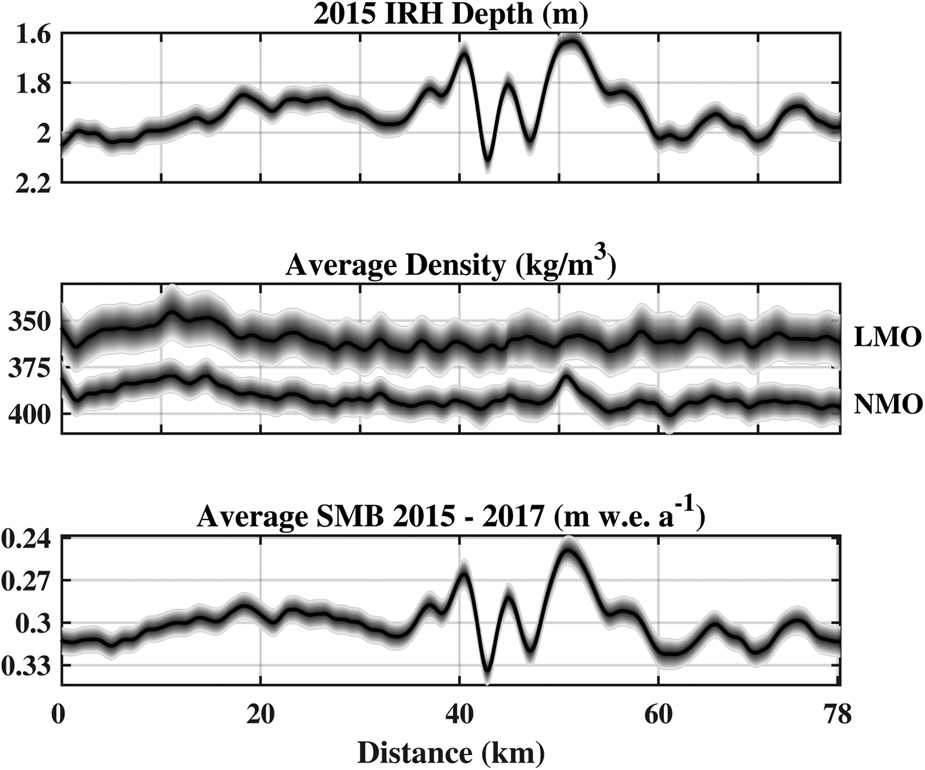
Fig. 5. The MxRadar inversion parameter distributions along GTC15 Spur West. The LMO and NMO densities were independently estimated and strongly correlate (R 2 = 0.67, p = 0). The MxHL model is parameterized by the average of the LMO and NMO densities, the 2015–2017 average SMB and MERRA (1979–2012) average 2 m temperature.
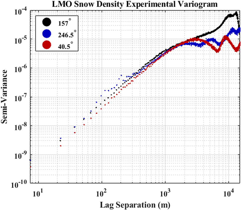
Fig. 6. We calculated experimental variograms of the LMO estimated snow density along the three azimuths of GTC 15 Spur West using lag separations up to 15 km. Plotted in log-log space, the linearity of each variogram slope indicates that spatial correlation among the three azimuths exists up to ~2 km distance. Correlation beyond this distance is difficult to assess given the limited azimuths and lag separations possible for GTC 15 Spur West. However, predominant wind direction appears to have a control on the correlation length, as evidenced by the $\gtrapprox 6\, {\rm km}$ range of the 157° transect variogram (in the direction of the predominant wind) and shorter, ~2 and ~3 km ranges of the 246.5° transect (orthogonal to the predominant wind) and 40.5° transect (oblique to the predominant wind), respectively.
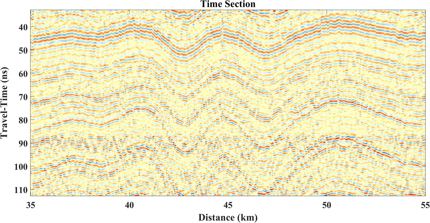
Fig. 7. Conventional GPR processing was applied to each of the nine constant offset radargrams. We then performed NMO correction to project each constant offset image to zero offset. We stacked the NMO corrected radargrams together to synthesize one conventional GPR travel-time image. The travel-time image remains quite noisy, and it is difficult to interpret due to the discontinuities along the reflection horizons.

Fig. 8. The travel-time image (Fig. 7) is first transformed into the stratigraphic age domain, known as the Wheeler (Reference Wheeler1958) domain. Then we applied structure-oriented filtering to the Wheeler domain image and converted into the depth domain. The depth section, taken from GTC15 Spur West, has remarkable continuity along the reflection horizons, which allows us to interpret IRHs to ~22.5 m depth. The undulation in the firn stratigraphy is caused by spatial variability in snow accumulation. It is necessary to interpret along steeply varying undulations like these to evaluate high resolution (< 5 km) regional climate model simulations of SMB. However, without the structure-oriented filter we would be unable to track the reflection horizons along the undulations.

Fig. 9. The GTC15 and MxHL historical SMB for January 1984–January 2017. Uncertainty in GTC15 SMB (± σ) was estimated following Graeter and others (Reference Graeter2018). Uncertainties in the MxHL 1984–2017 SMB (± σ) were propagated by Monte Carlo simulations of firn models generated from the parameter distributions of snow density, 2015–2017 SMB, and MERRA temperature. We applied ± 31 days uncertainty to the measured ages of isochrones within the simulations.
5. Discussion
We independently assessed the four sources of uncertainty in the MxHL SMB (depth, density, temperature and age) and then propagated these uncertainties through the MxHL model by Monte Carlo simulation to estimate the SMB mean and standard deviation for each year of 1984–2017. On average, the difference between GTC15 and MxHL SMB is small enough to accept the MxHL measured-modeled densities in place of extrapolating the measured firn core density along GTC15 Spur West. Extrapolated densities are likely to be much less accurate farther from core sites and in the percolation zone, due to increased near-surface pore space reduction caused by melt water infiltration (Harper and others, Reference Harper, Humphrey, Pfeffer, Brown and Fettweis2012). We also expect the accuracy of the HL density model to break down at elevations within the percolation zone (Brown and others, Reference Brown2012). Annual fluctuations in density, and density excursions due to warming events, are not captured in the HL model. Using the MxRadar, we have the ability to measure the density profile in the percolation zone with additional layer picking for near-surface velocity analysis, but the NMO approach is sensitive only to the average density of intervals in between the layer picks (Dix, Reference Dix1955) and is susceptible to errors due to subsurface velocity heterogeneities and data noise (Al-Chalabi, Reference Al-Chalabi1974).
In the upper ~2 m of the firn column, we replaced modeled densities with a linear fit between the two radar measurements of snow and firn density using the surface wave and the reflection from the fall 2014 IRH. This reduced the near-surface bias present in the HL density profile and we found strong correlation between the densities of these independent radar measurements. The richness of the MxRadar data stream permits geostatistical analysis at the sub-kilometer scale. We found that local (on the order of 1 km neighborhood) processes control the GrIS dry snow density. The similarity in spatial patterns of radar estimated surface snow density, up to ~2 km lag distance, contrasts with the findings that no correlation exists between surface snow density, latitude, longitude or elevation (Fausto and others, Reference Fausto2018), which is likely due to the limited observations of snow density at the <1 and <10 km scales within the Surface Mass Balance and Snow Depth on Sea Ice Working Group dataset (Montgomery and others, Reference Montgomery, Koenig and Alexander2018). Our variogram analysis was tested to 15 km lag separations along three azimuths: 157°, 246.5° and 40.5°. In the direction of the prevailing wind, we found $\gtrapprox 6\, {\rm km}$ correlation distance with diminishing correlation length for transects increasingly orthogonal to the prevailing wind. We found that the SMB decreased with increasing slope on the leeward, 157°, transect, which corroborated the findings of Arcone and others (Reference Arcone, Spikes and Hamilton2005). We did not find trends in SMB with slopes of the 246.5°, and 40.5° transects, as these transects were approximately orthogonal and 21.5° oblique to the predominant wind direction, respectively. Future application of this method to the 4000 + km traverse will allow the exploration of surface density variations at much larger scales and at additional orientations relative to the prevailing winds.
The 2014–2017 SMB appears to be overestimated by MxHL, though the near-surface radar velocity analysis was focused on this range. We support the radar findings here with the understanding that firn samples recovered from these depths are susceptible to in situ losses due to their unconsolidated nature. The radar retrieval has a sample footprint of approximately ~25 m (twice the length of the antenna array) and is non-destructive, while the borehole diameter is ~8 cm and samples only one point in space. It is also likely that the age model is less accurate nearest the ice-sheet surface due to core sample loss; however, we sacrifice greater accuracy in the radar domain because of the limitations in our ability to interpret depth image. The fall 2014 horizon was the latest IRH measured in our analysis. Picking annual reflection horizons later than 2014, near the model boundary, created steep gradients in the numerical derivative required to estimate the SMB which yielded erroneous values.
We see evidence of the 2012 melt event (Nghiem and others, Reference Nghiem2012) in the filtered depth image (Fig. 8). At 3 m depth, the top of the reflection sequence represents January 2013, and at 4 m depth, the bottom of the sequence is January 2011. This IRH sequence expresses fading and discontinuity that, we hypothesize, is the result of 2012 melt water infiltration. Measured at GTC15, the 2011 annual layer has a melt feature percentage of $7.9 \%$ . However, melt water-induced firn densification does not explain the inaccuracy in 2010 MxHL SMB, as 2010 recorded $0 \%$
 melt feature percentage at GTC15. The MxHL density model is accurate within the 2010 annual layer, rather our estimate of the 2010 annual layer thickness is 22 cm thinner than measured at GTC15. This is the second largest error in annual layer thickness, only behind the 2015 layer which was estimated to be 24 cm thicker than measured at GTC15 because of the aforementioned issues in estimating SMB near the model boundary. The degraded image quality of the 2011–2013 IRH sequence inhibited our ability to interpret the age sequence accurately enough to define the annual layer thicknesses for 2011 and 2012. Instead, we relied on interpolation to approximate the thickness of these horizons. The leading source of error in the historical SMB reconstruction are inaccuracies in the age model that result from limitations in our ability to interpret the radar image, even after applying the structure-oriented filter.
The multidecadal average SMB for the period 1984–2017 at GTC15 has remained nearly constant. Yet, sinusoidal variability in SMB on the decadal time scale is apparent in the MxHL historical SMB reconstruction and is confirmed by GTC15 SMB. Decadal variability in the MxHL reconstruction would not be observable without the application of structure-oriented filtering and interpretation that permitted an accurate instantaneous SMB model. For GPR imagery expressing small or gradual SMB variability, it may be sufficient to apply the structure-oriented filter in the Wheeler domain without the steps of interpretation, age model corrections and image re-flattening (Section S.1.6). The snow density estimation component is unique to the multi-offset radar and integral in our ability to parameterize the HL model. However, the structure-oriented filtering can be applied to any GPR imagery of isochronous firn, provided a stratigraphic age model in the radar travel-time domain is used as a proxy for the firn structure.
Along GTC15 Spur West, we expect the largest errors due to firn advection to occur across the studied undulations (Figs 7 and 8), where the SMB gradient is largest and oscillating. The two undulations here represent the same feature observed on outbound and inbound traverses, and serve as a demonstration of the repeatability of the methods. In regions where the spatial gradient in SMB is dynamic or ice-sheet surface velocities are large, the advection of firn mass decreases the accuracy of radar estimated SMB. On Pine Island Glacier, with ice surface velocities on the order of 10–103m a−1, strain corrections applied to the accumulation model amounted to a $1 \%$ correction to the 1986–2014 average SMB (Konrad and others, Reference Konrad2019). Ice surface velocities along GTC15 Spur West are on the order of 10 m a−1 (Joughin and others, Reference Joughin, Smith and Howat2018), and therefore we accept a contribution of error that is an order of magnitude less than the uncertainty, by not applying corrections for the SMB due to advection.
6. Conclusions
GreenTrACS conducted the first multi-offset GPR traverse on the Greenland Ice Sheet, covering a total distance of 4436 km. We examined a 78 km section of the GreenTrACS 2017 traverse (GTC15 Spur West) to develop the methodology for multi-offset GPR wave velocity, imaging and uncertainty analyses to accurately quantify the surface snow density, average snow density, firn density, instantaneous SMB, annual SMB and multidecadal average SMB for the period 1984–2017. Using travel-time inversion of the radar waveforms, we continuously mapped Greenland snow density without manual observations of the snow. We found consistent spatial correlation of near-surface density for separations up to 2 km distance and evidence to support the prevailing wind direction as a source of correlation up to 6 km distance. We found significant correlation (R 2 = 0.67, p = 0) between near-surface snow density and average snow density of the upper 2 m. We demonstrated the use of the Herron and Langway (Reference Herron and Langway1980) model that was parameterized by the radar-derived snow density, radar-derived SMB (2015–2017), and MERRA 2 m air temperature, to estimate firn density and age. Our measured-modeled firn density in the dry snow accumulation zone accurately represents the firn core but can be performed continuously along a traverse in the field without destructive measurements. GreenTrACS Core 15 Spur West presented an interesting challenge because of spatial SMB variability that is enhanced by the surface topography. In the dry snow zone, the topographic effect induces undulations in the firn stratigraphy which steepen with depth, due to the persistence of increased accumulation. Folds in the firn stratigraphy are difficult to image clearly with conventional GPR processing methods. Using seismic interpretation methods, we facilitated structure-oriented filtering by utilizing the firn age model to determine the firn structure. In doing so, we furthered the application of the IRH theory, which is integral in SMB analyses conducted with radar imagery. This innovation enabled our interpretation of deeper (from 16.60 ± 0.04 to 20.15 ± 0.04 m at GTC15) and older (from 1991 ± 31 to 1984 ± 31 days) layers and permitted tuning the age model to a degree of accuracy which allowed us to derive instantaneous estimates of SMB which we averaged annually and multidecadally. Future work will include application of this methodology to the entire 4000 + km GreenTrACS traverse, with independent evaluation at the 16 core sites. To reduce the labor in interpreting the radar imagery of future work, it would be advantageous to model the firn age-structure using the kinematic wave equation (Ng and King, Reference Ng and King2011) to capture the advection process imprinted on the radiostratigraphy without having to interpret the Wheeler domain radargram. We picked horizons in the Wheeler domain as a necessary step in applying the structure-oriented filter to the GTC15 Spur West radargram. This interpretive process could be avoided by generating the relative age using the kinematic wave equation. Yet, this model requires an independent estimate of firn density and accumulation to satisfy the initial and boundary conditions. Deep learning techniques have been recently applied to seismic imaging that automate structure-oriented filtering and horizon interpretation problems. By generating synthetic seismograms from numerical structural models as training data (Wu and others, Reference Wu2020), relative stratigraphic age models have been recovered from real seismic data and used for automated isochrone horizon interpretation (Geng and others, Reference Geng, Wu, Shi and Fomel2020). The kinematic wave firn model could serve as a basis for generating synthetic radargrams to be used in a deep learning application for historical SMB reconstruction.
Supplementary material
The supplemental material for this article can be found at https://doi.org/10.1017/jog.2020.91
Data availability
The 2017 GreenTrACS multi-channel GPR data can be found at https://doi.org/10.18739/A21G0HT84. The MATLAB scripts used in this analysis are continually under development and can be forked from the github repository https://github.com/tatemeehan/GreenTrACS_MxRadar.
Acknowledgments
Greenland Traverse for Accumulation and Climate Studies was funded by the National Science Foundation Office of Polar Programs: Awards # 1417921 and # 1417678. Additional support of this work was awarded through the NASA Idaho Space Grant Consortium Graduate Fellowship and the STEM Student Employment Program through the U.S. Army Engineer Research and Development Center, Cold Regions Research and Engineering Laboratory. We thank Steve Arcone and an anonymous reviewer for their recommendations which improved the communication of technical aspects of this work and Journal of Glaciology Scientific Editor Shad O'Neel for his additional review of our manuscript which greatly improved its readability.


 Open access