

Introduction
Deposition of snow from precipitation and wind events initiates layering within seasonal snowpacks (Reference ColbeckColbeck, 1991). Following deposition, melt events and gradual crystal metamorphism modify the layer properties. Detectable differences in properties such as density, grain size and texture define the layers of snow. These properties typically vary more between layers than within layers, yet there can also be a surprising amount of lateral variability (Reference Sturm and BensonSturm and Benson, 2004), either as a result of initial deposition or as a result of subsequent metamorphism. Stratigraphy, a term originally used in reference to layered sedimentary rocks, is used here to represent all of these aspects of the snow cover, and in particular the vertical sequence and lateral variation of snow layers with perceptible differences.
A high degree of lateral heterogeneity is particularly common in the snow cover of the windy tundra regions. Reference Sturm and BensonSturm and Benson (2004) presented stratigraphic observations at the 5 m–100 km scale and suggested that layer variability in seasonal snowpacks increased up to a length scale of about 100 m, whereupon it remained relatively constant through scales up to 100 km. Mechanical properties showed as much variability at the metre scale as the kilometre to tens of kilometres scale (Reference Sturm and BensonSturm and Benson, 2004). In deeper alpine and maritime snowpacks, detailed stratigraphic measurements at length scales of 5–10 m are limited, but snow micropenetrometer measurements from the Swiss Alps indicate that while lateral heterogeneity is more limited, it is still present (Reference Kronholm, Schneebeli and SchweizerKronholm and others, 2004).
The spatial variability of stratigraphy in seasonal snow-packs has important implications for remote sensing, hydrology and avalanche forecasting. Complex snow physics models such as SNTHERM (Reference JordanJordan, 1991), SNOWPACK (Reference Bartelt and LehningBartelt and Lehning, 2002) or Crocus (Reference Brun, David, Sudul and BrunotBrun and others, 1992) can be used to estimate the stratigraphy in order to calculate snow properties and energy fluxes at a point. Applied at several points, they can in principle be used to delineate stratigraphic heterogeneity, though in practice this would be cumbersome and extremely difficult.
Similar difficulties impact both passive and active microwave remote sensing used for monitoring snow; they are sensitive to not only variations in snow depth, but variations in stratigraphy, grain size and ice layers (e.g. Reference Durand, Kim and MargulisDurand and others, 2008). Active radar in the microwave frequency range has been shown to be sensitive to snow layer boundaries in studies dating to the late 1970s (Boyne and Ellerbruch, 1979; Reference Gubler and HillerGubler and Hiller, 1984), and since that time has become more portable (Reference Marshall and KohMarshall and Koh, 2008) and has been used for time-series measurements (Reference Heilig, Schneebeli and EisenHeilig and others, 2009). Some operational satellite sensors have high spatial resolution (e.g. TerraSAR-X at 2–10 m (Reference Hajnsek and EinederHajnsek and Eineder, 2005)), while ground-based radars and radiometers have pixel resolutions ranging from tens of centimetres to tens of metres (Reference Rees, Derkson, English, Walker and DuguayRees and others, 2006; Reference HardyHardy and others, 2008; Reference Marshall and KohMarshall and Koh, 2008). High-resolution field observations are thus increasingly important for understanding the integrated effect of heterogeneous snow stratigraphy on sensor response.
Reference Pielmeier and SchneebeliPielmeier and Schneebeli (2003) provide a comprehensive overview of the development of techniques used to quantify and record snow stratigraphy. The state of the art in 2003 was little different than when scientific observations of snow began: handwritten stratigraphic profiles of snow properties derived from manual measurements (Reference ColbeckColbeck and others, 1990). Recording snow stratigraphy at centimetre resolution over lateral distances up to 10 m was rare because of the time-consuming task of measuring multiple profiles within the trench (Reference Sturm and BensonSturm and Benson, 2004). Here we focus on a method for efficiently and objectively documenting snow stratigraphy on the centimetre scale over lateral distances of several to tens of metres.
Our method is based on near-infrared (NIR) photography. The reflection of light in the NIR wavelengths (750–1400 nm) is predominantly sensitive to snow grain size (Reference Dozier, Schneider and McGinnisDozier and others, 1981; Reference Haddon, Schneebeli, Buser, Frost and McNeilHaddon and others, 1997). With this as a basis, Reference Matzl and SchneebeliMatzl and Schneebeli (2006) used digital NIR images to compute the specific surface area (SSA) of snow grains within layers. They recognized that excellent stratigraphic profiles were produced by the photography, but did not focus on this aspect of the technique. Building on the recognition that NIR photography can record the snow stratigraphy in an efficient manner, we have developed a practical field protocol for recording layer height and thickness. Furthermore, we have extended the technique from producing simple pit-wall stratigraphy to objectively capturing the lateral variability in layers over distances of 10 m or more. This allows for extrapolation of properties like grain size and density to the 10 m length scale, which, in many environments such as the Arctic tundra, captures most of the variability that exists at the regional scale (Reference Sturm and BensonSturm and Benson, 2004).
Location
The methods and protocols described below were developed while working on the tundra snow cover near Toolik Lake, Alaska (68°38′ N, 149°36′ W). This snow cover has been described by Reference BensonBenson (1969), Reference ListonListon (1986) and Reference Benson and SturmBenson and Sturm (1993). The tundra snow cover includes depth hoar, wind slab, new and recent snow, and often layers of fine-grained snow. Thus, techniques applicable to it should be widely applicable in other classes of snow. The data we present come from a 10 m long trench excavated on 23 February 2008 in a snowdrift that had formed on flat lake ice.
Field Methods
The trench was cut using snow saws and knives to produce a smooth planar face. Rounded wooden blocks and soft brushes were then used to remove any artefacts resulting from the cutting process. A tape measure was placed along the base of the trench for georeferencing. A 4 m long aluminium rail with adjustable tripods on each end was positioned parallel to the trench face and about 1 m away. A Fuji S9100 digital camera, which was converted to allow both visible and NIR wavelengths to access the charge-coupled device (CCD), was mounted on a tripod head that slid along the rail. An XNite85058 filter, which has a peak wavelength transmittance between 870 and 940 nm (http://www.maxmax.com/aXNiteFilters.htm), was used on the f2.8 28–300 mm zoom lens. One advantage of the Fuji S9100 is that the monitor on the rear of the camera can be pivoted so that it can be viewed from above, which is highly advantageous for focusing and composing an image in the confines of a narrow trench (Fig. 1).
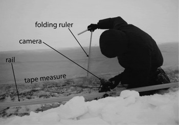
Fig. 1. The rail system in a snow trench on Toolik Lake. The tripods supporting each end of the rail are out of the picture to the left and right.
Each section of the trench was photographed three times: the first time with a note card indicating the position along the trench, the second time with a vertical ruler held flush to the face, and the third time with nothing obstructing the face. The ruler provided scale and improved the autofocus performance of the camera. Manually focusing the camera using distances marked on the focus ring (when present) is also feasible. The camera and trench were shaded, so that the trench face was diffusely illuminated by ambient light. Images were acquired in raw format with 28 mm focal length, an aperture of f2.8, autofocus, and a 2 s timed delay for the shutter release to minimize camera shake. Once triplicate photos were taken, the camera was slid laterally along the rail about 35 cm, ensuring a 30% overlap of subsequent photos down the trench face.
For purposes of comparison, standard manual strati-graphic profiles were made every 0.2 m along the trench, producing a total of 357 layer observations. At three positions along the length of the trench the density of each snow layer was measured using a 100 cm3 cutter and a digital scale.
Lens Calibration and Image Rectification
Most lenses produce image distortion that must be removed before quantitative measurements of geometry can be made. If we assume the CCD of the camera was parallel to the trench face, and a perfect rectilinear lens, then each pixel in the image will be equal to a fixed area of the trench face, independent of the location of the pixel in the image. However, lens barrel distortion creates a non-linear relationship between pixels and corresponding areas of the trench face. In certain applications this distortion can be ignored (Reference Matzl and SchneebeliMatzl and Schneebeli, 2006), but the lens used in our study produced up to 2.5 cm of distortion.
To rectify the lens distortion, firstly, the nodal point in the lens, where there is no parallax, was determined. A Panosaurus panoramic tripod head (http://gregwired.com/pano/Pano.htm) allowed the camera to rotate about the nodal point in the lens. Fore- and far-ground parallel vertical lines (e.g. a light pole and a building edge) were photographed. Then the camera was rotated and the gap separating the two lines was photographed multiple times as it appeared in different parts of the image. The camera pivot point was then moved forward or backward along the axis of the lens, and this process was repeated until the variation in the width of the gap was minimized. The camera could then be said to be rotating about the nodal point of the lens. Next, a level 360° panorama was shot with >30% overlap between images. Images that made up the panorama were loaded into commercially available software (PTGui), and control points in overlapping images were automatically selected. Foreground control points were removed to avoid parallax errors resulting from minor nodal point error. By viewing the pixel distances between the same objects as they appear in different portions of separate images (control points, n = 153), and by knowing that the entire panorama is 360° (a great circle on the celestial sphere), the angular distortion in every portion of the resulting image was inferred and removed using a fourth-order polynomial (example equation below). The parameters required to remove the distortion were saved for the specific lens and used to rectify each image from the trench.
To assess the error in rectification, a precise and regular 4 cm grid of squares was photographed perpendicularly. Before applying the lens distortion algorithm, the error for both vertical and horizontal distances ranged from 0 cm in the centre and corners of the image to 2.5 cm furthest away from those control points. After applying the fourth-order polynomial (distortion removal) to the image, errors were reduced to <1 mm throughout the image. As an example, the polynomial for the Fuji zoom lens at 28 mm was:

where r uncor is the radius between the initial selected pixel and the center of the image, and r cor is the radius between the corrected pixel and the center of the image. r uncor and r cor are scaled so that the value 1 corresponds to the maximum radius of both images. The difference between r uncor and r cor is zero at the center and corners of the image (r = 0, 1) and greatest about halfway between the center and corners (r ∼ 0.5).
Removing the ‘Bright Spot’
Our NIR images were brighter near the centre of the image than the edges, an artefact of the NIR filter and CCD construction. Other NIR cameras we used have had similar ‘bright spots’. The bright spot, which is similar to the more familiar vignetting (Reference AdamsAdams, 1980), caused pixel intensity errors of up to 12% and had to be removed to reduce gross artificial variations in intensity.
To remove the bright spot, an intensity adjustment matrix was developed. A photo was taken of an overcast sky to simulate a flat field. The pixel intensities in the flat field image were smoothed using a simple averaging filter of 28 × 28 pixels (1 × 1 cm) to remove high-frequency noise. Using a technique called pixel division, each pixel (i, j) in the uncorrected images (NIRuncor) was then normalized by multiplying by the mean flat field intensity ![]() , and then dividing by the corresponding pixel in the smoothed flat field image (FF), thereby producing images corrected for the white spot (NIRcor) (Fig. 2):
, and then dividing by the corresponding pixel in the smoothed flat field image (FF), thereby producing images corrected for the white spot (NIRcor) (Fig. 2):
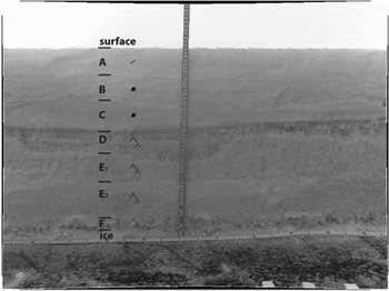
Fig. 2. An example NIR image of one section of a snow trench, with the layers indicated. The distortion and ‘bright spot’ have been removed. The black border is a result of the distortion removal.
Georeferencing
After the lens barrel distortion was removed from individual images, the images were considered to be planar, and were then aligned so that layer boundaries could be identified along the length of the trench. The 10 m tape measure running along the base of the trench was used to assign known locations to pixels in individual images (control points), so that images could be georeferenced. Control points were established by selecting 80 cm marks on the horizontal tape and the vertical ruler in the image and assigning each mark an x-y coordinate. A linear transformation was calculated relating the distance between control points along the tape to the number of pixels between corresponding control points in each image. The mean centimetre to pixel relationship was 0.02 cm per pixel, and locations calculated from the images had a very low rootmean-squared error (RMSE) of 0.07 cm. The centimetre to pixel relationship will vary from trench to trench depending on the distance between the camera and the wall.
We sought to accomplish the georeferencing using as few control points as possible for the desired accuracy. To determine the minimum number of control points for accurate georeferencing, in each image 2–10 cm marks were selected randomly from an 80 cm length of trench 100 times. Even when only 5 cm marks were selected, the RMSEs of the pixel to centimetre transformation were all less than 0.3 cm. This suggests that the pixel to centimetre transformation was robust and that despite subtle deviations from an ideal protocol that are imposed by the constraints of fieldwork, NIR images can be georeferenced with accuracy similar to, if not greater than, traditional in situ observations. This also indicates that the lens distortion has been accurately removed, and that pixels in the corrected image can be used to accurately measure distances in the trench face.
With only knowledge of the field-identified stratigraphy from the profile at the 0 m position along the trench (as an observer would obtain from a standard snow pit), layer boundaries were estimated from the NIR images throughout the 10 m trench, every 0.2 m where manual observations were made. To avoid bias, layer identification from the NIR trench image was performed by a different observer (Rutter) than the one who performed the layer identification in the field (Tape). The cursor was placed on the screen at the boundary between layers, and a digitizer was used to record the corresponding pixel coordinates in the digital image. Each vertical profile took about 5 min to delineate layer boundaries, making the total time for delineating stratigraphy in the trench image about 4.25 hours. The time required to delineate layers decreases with practice.
Results and Discussion
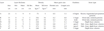
Field- identified stratigraphy showed seven snow layers (each assigned a letter) evident (sometimes discontinuously) throughout the trench (Fig. 2; Table 1). The top layer was 1 day old snow (A), and this was underlain by 2 day old soft wind slab (B). The subsequent layers were wind slab topped by melt crust (C); depth hoar (D); slab→hoar, defined as ‘a compact layer of snow exhibiting the cohesiveness of a wind slab but consisting of snow grains with kinetic growth features and depth-hoar grains’ (Reference Sturm and ListonSturm and Liston, 2003) (E1); a slab→hoar layer with larger grains, less dense than E1(E2); and, at the base, a layer of depth hoar with large crystals (F). The transition from A to B was subtle because both layers were soft recent snow. The melt crust that separated B and C was easily identified due to the change in hardness from overlying recent snow (B) to hard melt crust and slab (C). Layer boundaries above and below the internal hoar layer (D) were clear. The transition from slab→hoar to large-grained depth hoar (E1–F) was less distinct and sometimes gradational.
Table 1. Summary of field measurements of layers, densities and structure along the 10 m trench. Two density measurements were made per layer at 0, 5 and 10 m in the trench
The median difference between field- and image-identified layer boundary height was <2 cm (Fig. 3). For 75% of the image-identified boundaries, the difference was <1 cm (Figs 3 and 4). The image-identified layer accuracy was thus excellent when compared to field-identified layers that had a resolution of ∼1 cm. The NIR imaging boasted ease of collection and analysis at 1 cm horizontal resolution compared to what would have been required to produce that resolution using traditional methods.
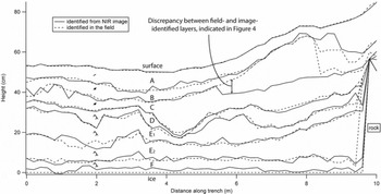
Fig. 3. Field- and image-identified stratigraphy over the 10 m trench, with layers indicated.
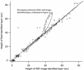
Fig. 4. Differences between the height of layer boundaries identified in the field and those identified from NIR images. R 2 = 0.97 between data and y = x line, the latter of which represents perfect agreement between field- and image-identified layer boundaries.
The snow-surface–air boundary was the easiest to estimate using NIR photographic methods. Beneath the snow surface the easiest boundaries to estimate from the trench image were those above and below the hoar layer (D) (Fig. 5). The layer boundaries from melt and wind-slab grains (C) to hoar (D), and from hoar (D) to slab→hoar (E1) were distinct because there were large differences in grain size and type. Identification and accurate estimation of the size and horizontal continuity of structurally weak layers, such as the internal hoar layer (D), was an important application of this method.
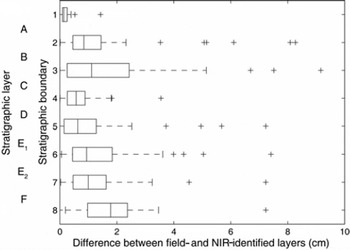
Fig. 5. Differences in the height of layer boundaries identified in the field and those identified from NIR images.
Where grain sizes and types were similar between layers (B–C and E1–E2) the layer boundaries were more difficult to estimate. A soft parting in the middle of layer C from 6 to 8 m was mistaken during image identification for the top of the layer (Figs 3 and 4). The base of the snowpack was the hardest boundary to pick from NIR images because the boundary between the base of the snowpack and the underlying lake ice was obscured by collapsed depth hoar in the lowest layer.
The comparatively larger errors in NIR boundary identification between wind slab (B: 356 ± 16 kg m−3) and dense wind slab (C: 411 ± 10 kg m−3) reaffirm the low dependence of NIR wavelengths on density (Reference Warren and WiscombeWarren and Wiscombe, 1980; Reference Grenfell and WarrenGrenfell and Warren, 1999), at least in cases like ours, where snow densities were <650 kg m−3 (Dozier, 1992). Consequently, despite this advance in the use of NIR imaging, the methodology here does not provide a direct observation of density. However, by extrapolating point measurements of density, which vary little across the trench (Table 1), to layers quantified by NIR, centimetre-scale variation of bulk density can be inferred along the length of the trench. Because illumination of the snow profile was not homogeneous, and no reflectance targets as reference were put on the wall, SSA and optical grain size can also not be quantified with this method. Nonetheless, as is the case for density, by extrapolating point measurements of grain size along layers quantified by NIR, centimetre-scale variations in vertically averaged grain size can be inferred.
NIR photography is not sufficient to replace field measurements of, say, density or hardness. NIR photography is an essential complement to field measurements, whether it is used to record stratigraphy in snow pits or snow trenches. The method proposed here is most useful to objectively record stratigraphy at sub-centimetre resolution. Once the 10 m trench has been excavated, the preparation of the trench wall and imaging using the rail system requires 45 min. It then takes about 2 hours of image processing to produce the stitched trench image. The time to identify the layers to produce the high-resolution stratigraphy for a 10 m trench is about the same in the office as in the field, and depends on the desired horizontal resolution. The NIR technique, however, boasts a record that is much more objective than the symbols produced by the traditional method. This makes the NIR method particularly advantageous in situations where multiple observers are involved in the same study.
Conclusion
We have expanded a recently introduced NIR photography technique (Reference Matzl and SchneebeliMatzl and Schneebeli, 2006) into a practical methodology describing the field acquisition of overlapping images and post-processing methods required for quantitative estimation and analysis of snow stratigraphy. In a shallow snow trench on lake ice, images were acquired that recorded stratigraphic variability. The high resolution (0.02 cm) and low error (0.3 cm) of georeferenced NIR images allow layer boundaries to be estimated with a median difference of <2 cm compared to field observations. NIR images also permit objective layer identification and analysis at <1 cm lateral resolution, whereas traditional field techniques are extremely tedious at this scale. The high-resolution stratigraphy can then be used to extrapolate profile measurements of grain size and density. Estimation of the thickness and horizontal continuity of structurally weak layers is also an important application of this method.
Acknowledgements
We thank J. Holmgren, K. Elder, D. Cline and the winter crew at the University of Alaska Fairbanks Toolik Lake research facility for technical and logistical support. M. Schneebeli provided valuable insights toward the development of this method. Financial support through UK Natural Environment Research Council (NERC) Fellowship NE/E013902/1 (to N.R.) and NASA THP/NEWS NNG06GE70G (to H.-P.M.) is gratefully acknowledged.
Additional Material
A ‘cheat sheet’ outlining the technique presented here can be requested from N. Rutter.


