


1. INTRODUCTION AND AIMS
Icelandic glaciers and ice caps are highly sensitive to atmospheric warming, and since the late 20th century, the rate of mass loss has, therefore, been substantial (Pálsson and others, Reference Pálsson2012; Björnsson and others, Reference Björnsson2013; AMAP, 2017). This relatively high sensitivity to variations in climate is due to Iceland's position in the North Atlantic Ocean, which places Iceland at the boundary of the polar and mid-latitude atmospheric circulation cells, converging warm and cold ocean currents, and directly in the path of cyclonic westerlies that are driven by the North Atlantic Oscillation (Björnsson and Pálsson, Reference Björnsson and Pálsson2008; Pálsson and others, Reference Pálsson2012; Björnsson and others, Reference Björnsson2013). In particular, the warm Irminger Current, which travels from the south-western coast of Iceland to the northern coast of Iceland contributes to Iceland's temperate maritime climate (Vilhjálmsson, Reference Vilhjálmsson2002).
Iceland has six major ice caps, which account for 90% of its permanent ice cover (Foresta and others, Reference Foresta2016). From October 2010 to September 2015, these ice caps lost mass at a rate of 5.8 ± 0.7 Gt a−1 (Foresta and others, Reference Foresta2016). However, this rate of mass loss was 40% lower relative to the previous 15 years (Foresta and others, Reference Foresta2016). This was, in part, due to a year of anomalous positive mass balance for Vatnajökull, Iceland's largest ice cap, in 2014/15 (Foresta and others, Reference Foresta2016). Owing to its size, changes in the mass of Vatnajökull can dominate the mass-balance signal of Iceland, and can contribute considerably to sea-level rise.
Vatnajökull is situated in south-east Iceland, and its mass loss is thought to be exacerbated by the development of lake-terminating outlet glaciers, which can accelerate terminus retreat through calving activity (Schomacker, Reference Schomacker2010). Here, the development of proglacial lakes is facilitated by the presence of marked over-deepenings that underlay numerous retreating Icelandic glaciers (Schomacker, Reference Schomacker2010; Magnússon and others, Reference Magnússon, Pálsson, Björnsson and Guðmundsson2012). Examples of lake-terminating outlet glaciers that drain the Vatnajökull Ice Cap include Breiðamerkurjökull, Fjallsjökull, Skaftafellsjökull, Svínafellsjökull, Virkisjökull/Falljökull, Heinabergsjökull, Hoffellsjökull and Fláajökull. Nearly all of Vatnajökull's ice marginal lakes have expanded since 1995, and the size and number of these lakes is predicted to increase in the future due to climate warming (Flowers and others, Reference Flowers, Marshall, Björnsson and Clarke2005; Schomacker, Reference Schomacker2010; Aðalgeirsdóttir and others, Reference Aðalgeirsdóttir2011). For example, Jökulsárlón, Breidamerkurjökull's proglacial lake, expanded by 6 km2 between 2000 and 2009 (Schomacker, Reference Schomacker2010).
Lake-terminating outlet glaciers can lose mass through a number of additional mechanisms when compared to land-terminating glaciers. These additional mechanisms are influenced by interactions at the glacier-lake boundary, and include thermally induced melt, changes to the longitudinal stress regime, the formation of basal crevasses and force imbalances at the terminus (Benn and others, Reference Benn, Warren and Mottram2007; Carrivick and Tweed, Reference Carrivick and Tweed2013). These mechanisms often result in calving events. The timing, nature and magnitude of these calving events are controlled by a range of factors which are glacier specific (e.g. subglacial topography and glacier structures) and non-glacier specific (e.g. lake temperature) (Westrin, Reference Westrin2015).
An increase in the calving activity of a glacier can lead to the initiation of a number of positive feedbacks (Meier and Post, Reference Meier and Post1987; Van der Veen, Reference Van der Veen1996; Van der Veen, Reference Van der Veen2002; Vieli and others, Reference Vieli, Jania and Kolondra2002; Benn and others, Reference Benn, Warren and Mottram2007; Joughin and others, Reference Joughin2008; Carr and others, Reference Carr, Vieli and Stokes2013; Hill and others, Reference Hill, Carr, Stokes and Gudmundsson2018). For example, it can cause the glacier to retreat into deeper water, which will increase the buoyant forces acting on the terminus, increase torque and subsequently increase the rate of calving activity and associated retreat (Van der Veen, Reference Van der Veen1996; Van der Veen, Reference Van der Veen2002; Benn and others, Reference Benn, Warren and Mottram2007). In addition, a glacier terminus could begin to float as buoyant forces increase; this can reduce effective pressure at the ice-bed interface, and facilitate an increase in glacier velocities and longitudinal stretching (Van der Veen, Reference Van der Veen1996; Van der Veen, Reference Van der Veen2002; Benn and others, Reference Benn, Warren and Mottram2007). These changes may subsequently lead to thinning of the terminus, rendering it more vulnerable to fracturing and calving activity (Van der Veen, Reference Van der Veen1996; Van der Veen, Reference Van der Veen2002; Benn and others, Reference Benn, Warren and Mottram2007).
Proglacial lakes are becoming increasingly widespread globally (e.g. Iceland, Patagonia, New Zealand and the Himalaya), and can strongly enhance ice loss (Motyka and others, Reference Motyka, O'Neel, Connor and Echelmeyer2003; Bolch and others, Reference Bolch, Pieczonka and Benn2011; Dykes and others, Reference Dykes, Brook, Robertson and Fuller2011; Carrivick and Tweed, Reference Carrivick and Tweed2013). However, our understanding of the interactions between proglacial lakes and their adjacent glaciers are not fully understood (Benn and others, Reference Benn, Warren and Mottram2007; Carrivick and Tweed, Reference Carrivick and Tweed2013). This study aims to better understand the relationship between proglacial lake development, local climate, glacier dynamics and glacier structure at lake-terminating outlet glaciers by presenting a detailed analysis of the changing dynamic and structural regime of Fjallsjökull in response to variations in local climate between 1973 and 2017. Fjallsjökull and its proglacial lake Fjallsárlón are little studied, but the lake is the third largest proglacial lake in south-east Iceland, after Vatnajökull's two largest proglacial lakes attached to Breiðamerkurjökull (which have received significant scientific attention). We use satellite imagery from various platforms to calculate the change in terminus position, lake area, surface velocities and surface structures over time. From these data, we propose a conceptual model, which combines structural and velocity datasets, to explain the development of a distinctive ‘concentrated’ ice flow regime at Fjallsjökull.
2. METHODS
2.1. Study area
Fjallsjökull is located on the eastern side of the Öræfajökull ice cap, south-east Iceland (Evans and Twigg, Reference Evans and Twigg2002) (Fig. 1). The Öræfajökull ice cap occupies the caldera of Öræfajökull stratovolcano and is located on the southern side of the much larger Vatnajökull ice cap (Magnússon and others, Reference Magnússon, Pálsson, Björnsson and Guðmundsson2012; Phillips and others, Reference Phillips2017). Fjallsjökull descends from the south-eastern side of Öræfajökull, and is composed of a series of ice falls (Evans and Twigg, Reference Evans and Twigg2002) before terminating in Fjallsárlón, which had an area of 3.7 km2 in 2016 (Fig. 1). Fjallsárlón is located within a 3 km wide × 4 km long, c. 206 m deep overdeepening, which is being revealed in response to the westward lateral retreat of the margin of Fjallsjökull (Howarth and Price, Reference Howarth and Price1969; Magnússon and others, Reference Magnússon, Pálsson, Björnsson and Guðmundsson2012).
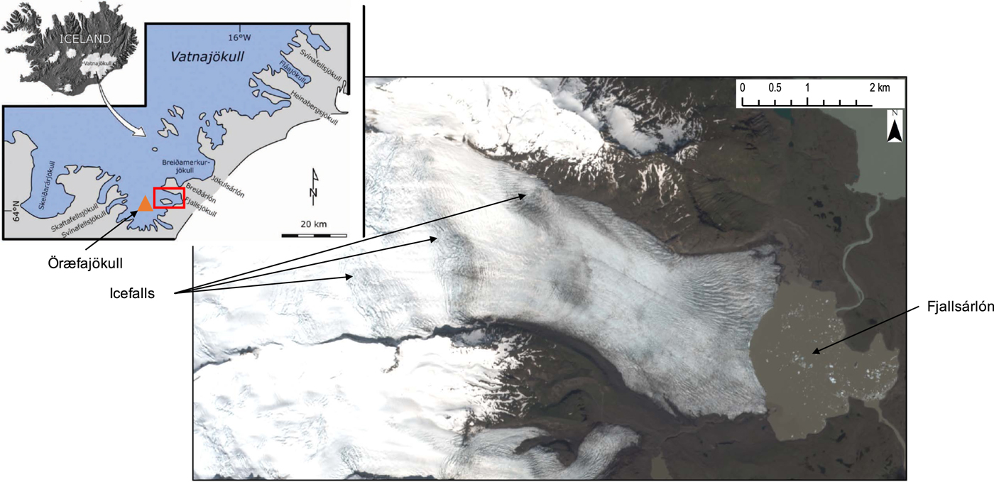
Fig. 1. A map of the study area, Fjallsjökull, in the context of Iceland and the south-east Vatnajökull ice cap (subset). The orange triangle in the subset image shows the location of Öræfajökull, and the red box indicates the extent of Fjallsjökull. Subset image source: modified from Schomacker (Reference Schomacker2010). Satellite image source: Sentinel 2 image from 6 June 2018 (downloaded from Earth Explorer).
2.2. Optical imagery
Twenty-eight remotely sensed optical images, including Landsat 1–8 (downloaded from: https://earthexplorer.usgs.gov), Sentinel 2 (downloaded from: https://earthexplorer.usgs.gov), Google Earth (downloaded from: the Google Earth Pro application), PlanetScope Imagery (https://www.planet.com) (Planet Team, 2017) and National Land Survey of Iceland Imagery (http://www.lmi.is/wp-content/uploads/2013/10/License-for-use-of-free-NLSI-data-General-Terms.pdf) were downloaded for the period between 1979 and 2018 (Table A.1). Imagery was downloaded if the area of interest was cloud free, and not obscured by scan line failures associated with the Landsat 7 ETM instrument. For the purpose of frontal position change and lake area change analysis, images were obtained for the summer months of July--September as these months had little snow cover, and regions could be mapped with greater accuracy (Table A.1 and Fig. S.1). To be sure that we were not picking up a signal from seasonal variation by using imagery across these 3 months, the terminus position was digitised from a July image (7 July 2015) and a September image (25 September 2015). The terminus position change between these two images was 9.9 m, which was within 0.1% of the minimum total error (geo-location error and digitisation error) associated with the Landsat 8 imagery. Images for structural mapping were obtained between June and August (Table A.1 and Fig. S.5). Images for feature tracking were selected with a minimum temporal gap of 11 months, to resolve velocity changes (Table A.2). This time gap was determined by visually assessing the offset of features between images within image pairs.
2.3. Frontal position change and lake area change
The rectilinear box method (e.g. Moon and Joughin, Reference Moon and Joughin2008; Lea and others, Reference Lea, Mair and Rea2014) was used to calculate frontal position change for 13 time steps between 1973 and 2016. This method was selected as it can account for asymmetric changes at a calving front (e.g. Lea and others, Reference Lea, Mair and Rea2014; Larsen and others, Reference Larsen2016). The width of the rectilinear box encompassed the maximum width of the lake-terminating portion of Fjallsjökull (identified in 2016), rather than the full width of the terminus. This approach minimised potential errors in accurately identifying the location of the land-terminating portion of Fjallsjökull, which is debris covered and is difficult to distinguish from its surroundings. This approach is further justified due to the study's focus on the impact of the lake on glacier dynamics and structural change.
Landsat 7 ETM and Landsat 8 OLI/TIRS images were pan sharpened using band 8, to produce a 15 m pixel resolution output in RGB. These images were then used to delineate the terminus position at a scale of 1:6000. For the Landsat 1-5 MSS images (60 m pixel resolution) and Landsat 4-5 TM images (30 m pixel resolution), the terminus was digitised at scales of 1:12500 and 1:10000, respectively (Table A.3). These scales allowed the accurate mapping of the terminus position and prevented images from becoming too pixelated for reliable interpretation (Lovell, Reference Lovell2016). To ensure that this approach did not affect the results, the terminus position for each satellite sensor type was digitised at the greatest spatial scale used (1:12500). Under 0.25% variation was found in both the mean terminus length and lake area relative to the original measurements using different scales.
Lake area change was quantified using the same imagery, time steps and digitising scale as frontal position change. At each time step, the lake boundary was manually digitised. Channels exiting the lake were excluded from the shape-file at the point of inflection (i.e. where the channel began to form). In addition, the proportion of Fjallsjökull's margin that terminated in Fjallsárlón was calculated over the study period, by dividing the length of the glacier margin that terminated in the lake by the full terminus length.
Two error sources are present with frontal position and lake area change calculations: manual digitisation errors and co-registration errors (Table A.4). The former was quantified by digitising the terminus position/lake area of Fjallsjökull for the different satellite image types, and calculating the mean difference in terminus position relative to the original measured value (Carr and others, Reference Carr, Stokes and Vieli2014). The latter was quantified by assessing the offset of each satellite image type relative to a base scene. For the purpose of this study, a Landsat 8 image was selected as the base scene, as the Landsat 8 images used had low geolocation errors (7.8–8.9 m RMSE) and scenes from this sensor were used throughout the study (Table A.4).
2.4. Ice surface elevation change
Changes in ice surface elevation were investigated using the Arctic DEM dataset which is available from the Polar Geospatial Centre (https://www.pgc.umn.edu/data/arcticdem). This dataset provides digital surface models (DSMs) for areas north of 60° from 2011 in some regions (Morin and others, Reference Morin, Porter, Cloutier and Howat2016). The Arctic DEM data have a spatial resolution of 2 m, and are typically downloaded as 17 km ×110 km strips (Barr and others, Reference Barr2018). However, at Fjallsjökull, few data strips covered the full region of interest, and data availability was therefore limited to 2012 and 2013. Once the DSMs were downloaded, they were resampled to 30 m resolution, to reduce the impact of crevassing on the calculated elevation change. The ‘minus’ tool was then used in ArcGIS to calculate the elevation change. The error associated with horizontal and vertical planes for the Arctic DEM data is 4 m.
2.5. Near-terminus velocities
Surface velocities at Fjallsjökull were calculated in the open-source feature tracking toolbox ‘Image GeoRectification and Feature Tracking’ (ImGRAFT) (http://imgraft.glaciology.net) using MATLAB (Messerli and Grinsted, Reference Messerli and Grinsted2015). Pre-processing steps included clipping all images to the same extent, to reduce the total processing time. In an attempt to increase the surface texture of the input images and increase the number of displacement retrievals (Fahnestock and others, Reference Fahnestock2015), a high pass filter was tested on images. However, it was found that this approach led to an increase in the number of false-positive retrievals for the flow orientation, and this step was, therefore, disregarded. Errors associated with the surface velocity calculations were quantified by taking the mean of five displacement values for stationary features (e.g. valley sides and arêtes) within each image pair (cf. Lea and others, Reference Lea, Mair and Rea2014). The average surface velocity error across all image pairs was between 0 and 10 m a−1. The only filter applied to the feature tracking results is a signal to noise ratio of 0.6.
Within ImGraft there are a series of processing parameters that can be changed including: template size (60 × 60 pixels); search image size (100 × 100 pixels); regular gridded points (5 × 5 pixels); and the signal to noise ratio (0.6) (Messerli and Grinsted, Reference Messerli and Grinsted2015). In this study these parameters were systematically adjusted to find the flow field that best fitted the following two criteria: (i) to minimise the number of flow directions orientated up-glacier, and (ii) minimise any extremely high values. Currently, there are no direct measurements or InSAR data of surface velocities at Fjallsjökull, and therefore it was not possible to compare the feature tracking results with pre-existing datasets. Owing to the higher spatial resolution of the PlanetScope Imagery (3 m), different template (300 × 300 pixels) and search region (500 × 500 pixels) sizes were applied to ensure that the algorithm could detect the full displacement over the time period. Gridded points of 20 × 20 pixels were also used, to minimise the computational time required.
2.6. Glaciological structures
Following the methodology outlined by Phillips and others (Reference Phillips2017) three detailed structural maps of Fjallsjökull's terminus were created for 1982, 1994 and 2011. These time steps were selected based on image availability, and because they provide an insight into the glacier's structural evolution on decadal timescales, which allows us to better understand the long term structural changes that have occurred at Fjallsjökull in response to climatic variations. Surface fractures were mapped at a scale of 1:500 for 1982 and 1994, and at a scale of 1:1000 in 2011. These scales were selected based on the resolution of the base images (Table A.3). The 2011 structural map provides a comprehensive overview of the most recent structural regime at Fjallsjökull, and extends 2.5 km up-glacier, whereas the 1982 and 1994 structural maps extend 0.75 km up-glacier, focussing on the structural development of the calving front. This approach allowed us to assess the glacier's wider structural composition in near-present day (2011). Fractures were grouped into domains based on variations in fracture orientation following Phillips and others (Reference Phillips2017). The orientation (strike) of the fractures were calculated using a Python script within ArcGIS (Diaz Doce, unpublished) and the data plotted as a series of rose diagrams using the software package Stereostat by Rockworks TM.
2.7. Meteorological data
Meteorological data were downloaded from the Icelandic Meteorological Office (http://en.vedur.is/climatology/data/) for 1973–2016. Daily air temperature data were obtained from two stations, Kvísker and Fagurhólsmýri, due to their close proximity to Fjallsjökull. Data were available from 1973 to April 2008 at Fagurhólsmýri, and from May 2008 to present at Kvísker. The measurements from these two stations were combined to produce a full time series of mean annual air temperatures over the study period (1973--2016). These data were used to calculate mean annual air temperatures, mean summer air temperatures (for June--August), and annual positive degree day (PDD) sums. To minimise the introduction of bias through missing values, years that were missing a month of data (2008 and 2010), and months that had fewer than 22 days of data, were excluded from further analysis (Carr and others, Reference Carr, Vieli and Stokes2013). Subsequently, mean summer air temperatures were calculated from the daily data for June, July and August. Annual PDD sums were calculated from the sum of the daily temperatures that were above 0°C for each year. Total annual precipitation data for 1973--2011 was downloaded from the Icelandic Meteorological Station at Kvísker.
2.8. Statistical analysis
‘Change-point’ analysis was conducted to test for statistically significant breaks in the terminus position data, lake area data and meteorological data (Eckley and others, Reference Eckley, Fearnhead and Killisck2011; Killick and others, Reference Killick, Fearnhead and Eckley2012; Carr and others, Reference Carr, Stokes and Vieli2017). This analysis was performed in MATLAB using the ‘findchangepts’ function, following Hill and others (Reference Hill, Carr, Stokes and Gudmundsson2018). The function used linear regression to identify significant breaks in each of the time series. Where the regression (intercept) and mean (slope) coefficients for the linear equation changed significantly at a data point, a change point was identified (Hill and others, Reference Hill, Carr, Stokes and Gudmundsson2018). The ‘maximum number of changes’ parameter was set to three, this ensures the test finds the three most significant change-points in the dataset. Without limiting the ‘maximum number of changes’, an arbitrary number of change-points is identified, and the function has the potential to identify a change-point between every data point.
3. RESULTS
3.1. Terminus position and lake area
The margin of Fjallsjökull retreated by 1.21 km between 1973 and 2016 (Fig. 2). Between 1973 and 1991 and 1994 and 1998 there was no discernible change in ice margin position. These periods were separated by a small (0.09 km) phase of retreat between 1991 and 1994 (Fig. 2). However, since 1998 the rate of ice margin retreat increased substantially and this higher rate was sustained for the remainder of the study period with a mean annual rate of 0.055 km a−1 (Fig. 2). Coincident with terminus retreat, lake area increased by 2.72 km2 between 1973 and 2016 (Fig. 2). From 1973--1991 and 1994--1998 there was no discernible increase in lake area, separated by a 0.17 km2 increase in area in 1991--1994 (Fig. 2). Since 1994, however, lake area increased by 2.42 km2. Importantly, the accelerated rate of terminus retreat in 2011--16 (0.06 km a−1) coincided with a period of relatively fast lake expansion (0.15 km2 a−1) (Fig. 2), and change-point analysis identified comparable changes in the terminus position and lake area datasets, in 2001, 2009 and 2011, respectively (Table 1).
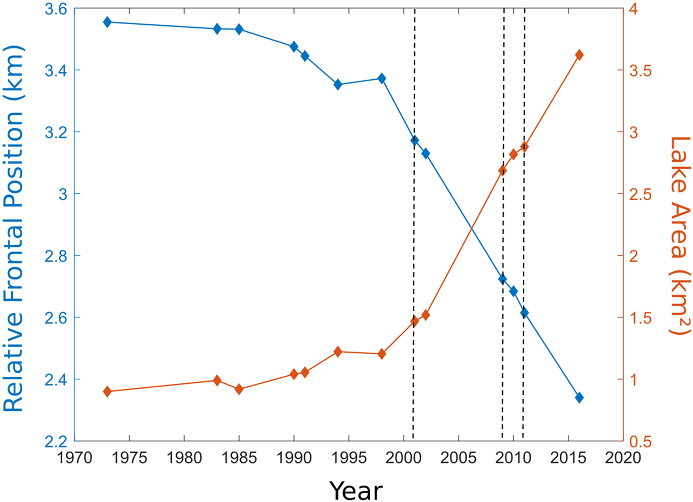
Fig. 2. Lake area and relative frontal position between 1973 and 2016. The vertical dashed lines indicate where statistically significant change-points were identified for both datasets.
Table 1. The statistically significant change-points identified for terminus position, lake area, atmospheric air temperatures, summer air temperatures, positive degree days and precipitation over the study period

3.2. Ice surface elevation change
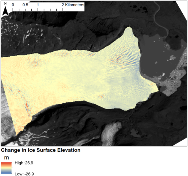
Between 2012 and 2013, Fjallsjökull underwent ice surface elevation changes ranging from −26.9 to 16.9 m (Fig. 3). Within 1.2 km of the calving front, a widespread thinning trend was observed, with the magnitude of thinning in crevasse free areas ranging from c. −4 m towards the glacier's lateral margins to c. −10 m towards the glaciers central axis (Fig. 3). Thinning was recorded up to 3 km up-glacier of the calving front, with the magnitude of thinning gradually decreasing to c. 1 m as the distance up-glacier increased. Above 3 km, the glacier's ice surface elevation predominantly increased by c. 1-2 m (Fig. 3).
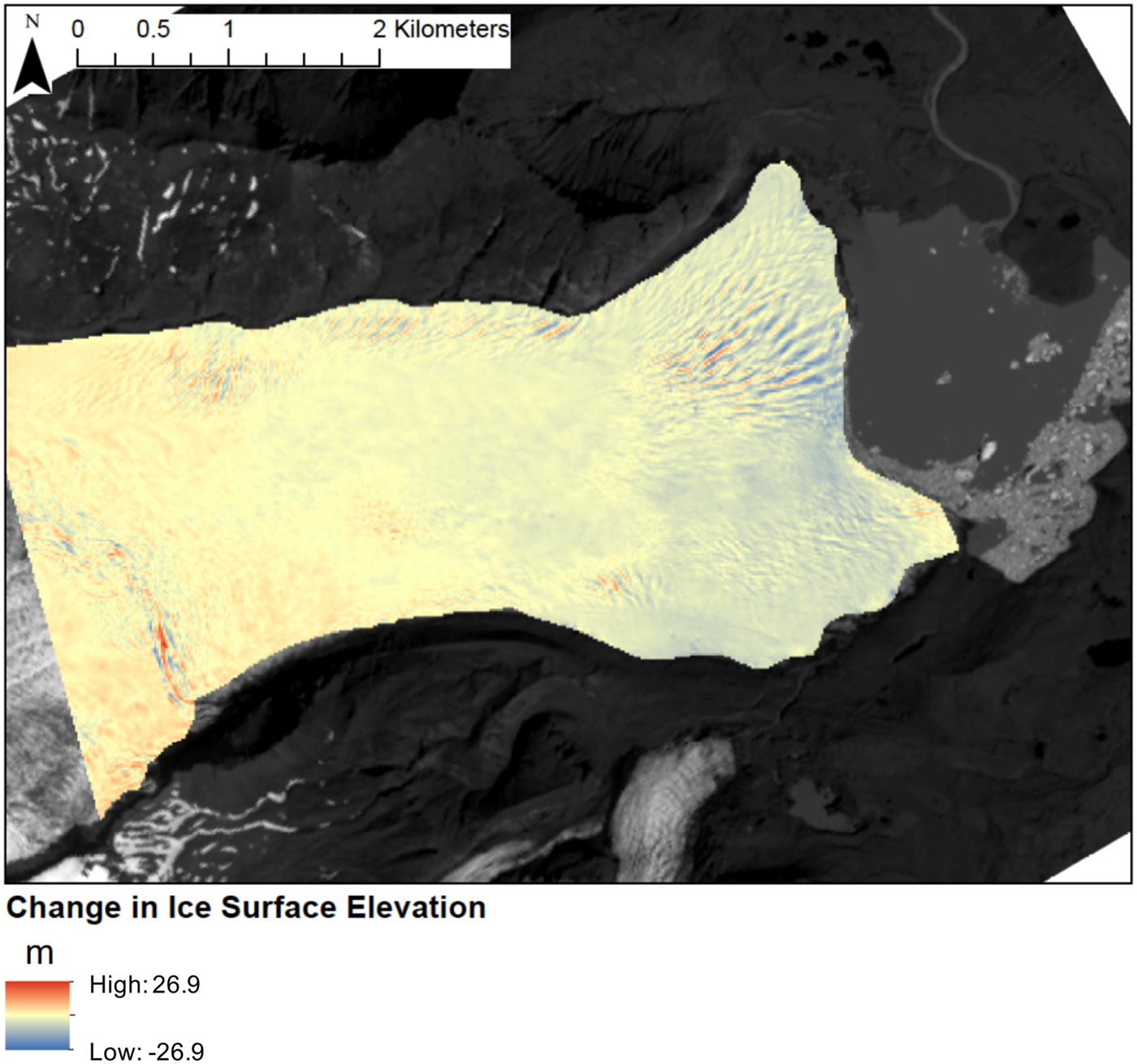
Fig. 3. Change in ice surface elevation at Fjallsjökull between 2012 and 2013, calculated using Arctic DEM digital surface models.
3.3. Climatic trends
Overall, mean annual 2 m air temperatures and mean summer 2 m air temperatures increased by 2.1 and 1.5°C, respectively, between 1973 and 2016 (Fig. 4). Mean summer air temperatures were highest in 2003 (11.1°C), 2014 (11.2°C) and 2016 (10.9°C). The mean annual PDD sum increased by 511.3 between 1973 and 2011, and peaked in 2014 at 2437.7 (Fig. 4). Change-points were identified in 1979 and 1992 for mean annual surface air temperatures, in 1984 and 2001 for PDD, and in 2015 for mean summer surface air temperatures (Table 1). Total precipitation varied greatly between years, although no obvious trends in the data were detected. Peaks in total precipitation occurred in 2002 (4630.3 mm), 2006 (4477.7 mm), and 2011 (4556.6 mm) (Fig. 4). Change-points in the precipitation data were identified in 1989, 2002 and 2010 (Table 1).
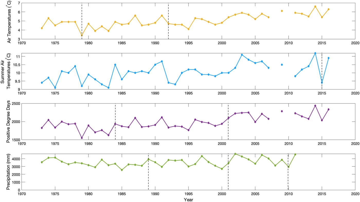
Fig. 4. Climate data showing mean annual air temperatures, mean summer air temperatures, positive degree days and total annual precipitation between 1973 and 2011. The vertical dashed grey lines indicate the change-points found within each dataset.
3.4. Glacier surface velocities
We observed marked increases in the average values and spatial complexity of glacier surface velocities in the period between 1990 and 2018 (Fig. 5). In 1990/91, surface flow was slow, and the flow directions were arranged in a radial fan-like pattern (Fig. 5a), typically equated with a plug-flow style of glacier movement as the ice spreads laterally to form a piedmont lobe. Towards the glacier's centre line, velocities ranged between 20 and 40 m a−1 (Fig. 5a).
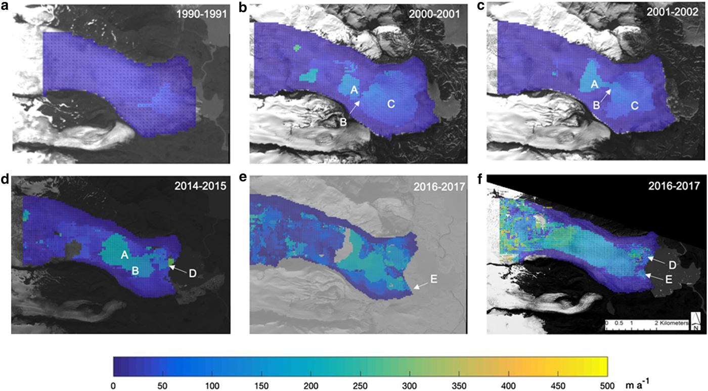
Fig. 5. Surface velocities at Fjallsjökull's terminus between 1990 and 2017. Labels i-v indicate notable features within the surface flow velocity fields. ‘A’ marks a distinct patch of relatively faster flow, ‘B’ marks a ‘corridor’ of ice flow, ‘C’ marks a laterally and longitudinally extensive area of relatively faster flow velocities, ‘D’ marks a northern ‘corridor’ of relatively faster flow towards the margin, and ‘E’ marks a southern ‘corridor’ of relatively faster flow towards the glacier margin. Sub-image 19a is based on calculations from Landsat 4-5 TM images, sub-images 19b and 19c are based on calculations from Landsat 7 + ETM images, sub-image 19d is based on calculations from Landsat 8 OLI/TIRS images, sub-image 19e is based on calculations from Sentinel-2 MSI images, and sub-image 19f is based on calculations from PlanetScope imagery (Planet Team, 2017). Larger individual figures for each of the velocity fields can be found in the Appendices (S.2–S.7).
However, between 1990/91 and 2000/01, there was a substantial increase in the spatial complexity and magnitude of surface velocities, and a pulse of high surface velocities migrated towards the margin of the glacier. Region ‘A’ indicates the origin of this pulse, a newly formed area of WNW--ESE trending relatively fast flow (170 m a−1) (Fig. 5b). This ice then migrated down-slope through region ‘B’ (a narrower region of relatively faster flow velocities), and eventually into region ‘C’ (a 2 × 2.3 km region of faster flow located adjacent to the glacier margin) (Fig. 5b). Within region ‘C’, velocities were much greater in the northwest (140 m a−1) relative to the northeast (80 m a−1) (Fig. 5c). External to these regions, velocities ranged between 0 and 40 m a−1 (Fig. 5b). Between 2000/01 and 2001/02, region ‘A’ (the origin of the relatively fast flowing pulse) had extended further, and covered 1.5 km of the terminus' width (Fig. 5c). In addition, region ‘B’, which acted as a ‘corridor’ for the fast flow velocities had migrated to a more central position, and calculated velocities were as high as 160 m a−1 (Fig. 5c).
By 2014/15, the surface velocities had further increased in magnitude and spatial complexity. Velocities in the origin region ‘A’ increased further, and peaked at 200 m a−1 (Fig. 5d), and region ‘B’ widened by 800 m. In addition, a fast flow corridor developed in the northern portion of the terminus (region ‘D’) which connected region ‘C’ to the calving front, and exhibited flow speeds between 100 and 200 m a−1 (Fig. 5d). Outside of the fast flowing regions, ice velocities at the land-terminating sections of the glacier were between 0 and 10 m a−1, and between 40 and 60 m a−1 at the lake-terminating portions (Fig. 5d). From 2014/15 to 2016/17, velocities in region ‘D’ increased. Furthermore, a new corridor of fast flow developed (region ‘E’) in the southern section of Fjallsjökull's terminus, trending in a WNW-ESE direction, with velocities between 110 and 200 m a−1 (Fig. 5e). Flow between these fast flow corridors was relatively slow, ranging from 20 to 100 m a−1 (Fig. 5e). Similar patterns were observed in 2017/18 as 2016/17, although slight (~5 m a−1) velocity increases were observed in each of the fast flow corridors (Fig. 5f).
Overall, Fjallsjökull's surface flow regime became increasingly complex between 1990 and 2018 (Fig. 6). Early data (1990–1991) show relatively slow flow velocities (0–30 m a−1) at the glacier's margin and moderate flow velocities (30–110 m a−1) towards the glacier's central axis (Fig. 6). Flow directions were arranged in a splaying pattern and flow directions within the glacier's central zone were directed towards the calving front (Fig. 6). In contrast, by 2016/17 and 2017/18, fast flow (≥110 m a−1) dominated the central portions of the terminus, and pulsed towards the glacier margin through two fast flow ‘corridors’, which extended from approximately 2.6 km inland to the calving front (Fig. 6). At the outer margins of the fast flow ‘corridors’ medium flow velocities typically dominated, orientated in the direction of the calving front (Fig. 6). However, with increasing distance from the fast flow ‘corridors’ and increasing proximity towards the glacier's lateral margins, there was a gradational reduction in flow velocities and change in flow orientation (Fig. 6). The glacier's lateral margins continued to exhibit the remnants of the slow (0–30 m a−1) splaying flow pattern recorded in 1990/91 (Fig. 6).
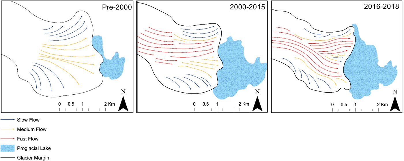
Fig. 6. A three-stage conceptual model of glacier evolution at Fjallsjökull, based upon changes in glacier dynamics and structural architecture. Stage 1 (Pre-2000) represents relatively slow flow velocities, arranged in a splaying pattern. Stage 2 (2000–15) represents an increase in flow velocities and the development of a fast flow ‘corridor’ in the north. Stage 3 (2016–18) represents the propagation of a secondary flow ‘corridor’ in the south of the terminus.
3.5. Structural architecture of fjallsjökull
Between 1982 and 2011 the structural evolution of Fjallsjökull was dominated by a transition from a radial fracture pattern towards a fracture pattern characterised by a series of dextral strike-slip faults. Furthermore, our results show structural evolution towards the calving front. These results support the surface velocity dataset, and further evidence the development of an increasingly concentrated flow regime, through which a pulse of relatively faster flowing ice migrated towards the terminus.
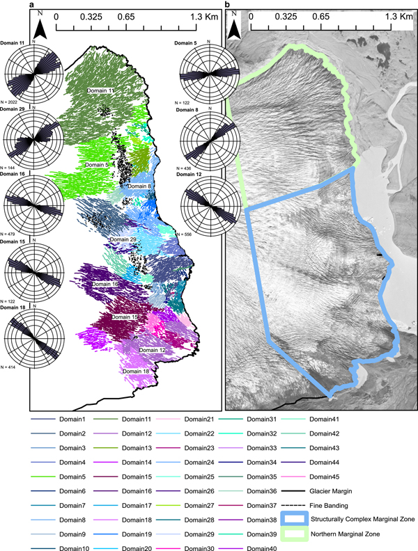
In 1982, the marginal zone of Fjallsjökull could be divided into 45 domains and two key structural zones: the Northern Marginal Zone and the Structurally Complex Frontal Zone (Fig. 7). The Northern Marginal Zone included Domains 5 and 11, which were characterised by arcuate, open (~3–5 m wide) fractures (crevasses) that formed a distinct splaying/radial pattern (Fig. 7). This splaying pattern was orientated W--E towards the centre line of the glacier, and NNW--SSE at its margin, as the orientation of the fractures reflected the lateral spreading of the ice within the piedmont zone of the glacier's terminus. The Structurally Complex Frontal Zone in 1982 comprised 41 individual domains, reflecting the structural complexity of this part of Fjallsjökull (Fig. 7). The majority of fractures within this area were weakly curved to straight, open features which were aligned parallel to the flow direction (WNW--ESE) of the glacier (e.g. Domains 12, 15, 16 and 18). In addition, a series of transverse to flow, arcuate fractures were also identified up to 300 m up-glacier of the calving front (Fig. 7). These fractures were predominantly open (~3–5 m wide), straight, steeply dipping, and closely spaced (e.g. Domains 8, and 29) (Fig. 7). Arcuate, up-ice dipping banding was also identified in 1982 (Fig. 8a). The banding comprised alternating dark and light layers (typical of Ogive banding), which was made of short (50--100 m long), and thin (1--10 m wide) segments (Fig. 8a). The banding was weakly crenulated, with fold wavelengths between 5 and 50 m, and amplitudes between 1 and 10 m (Fig. 8a).
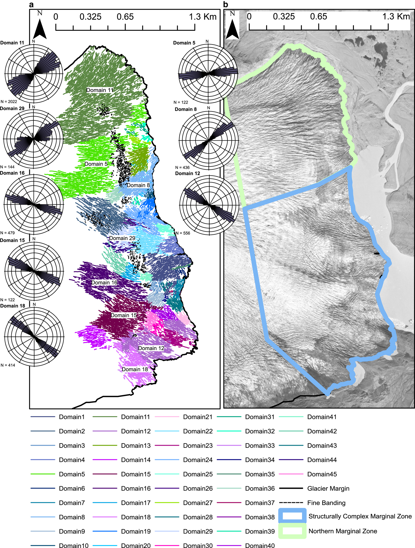
Fig. 7. Mapped surface structures at Fjallsjökull's terminus in 1982, key domains are labelled and are also represented by rose diagrams, (b) The corresponding aerial photo, from which the surface structures were mapped (acquisition date: 20 August 1982, obtained from: The National Land Survey of Iceland (http://www.lmi.is/wp-content/uploads/2013/10/License-for-use-of-free-NLSI-data-General-Terms.pdf)). A fully labelled high resolution version of this map can be found in the appendices (S.8).
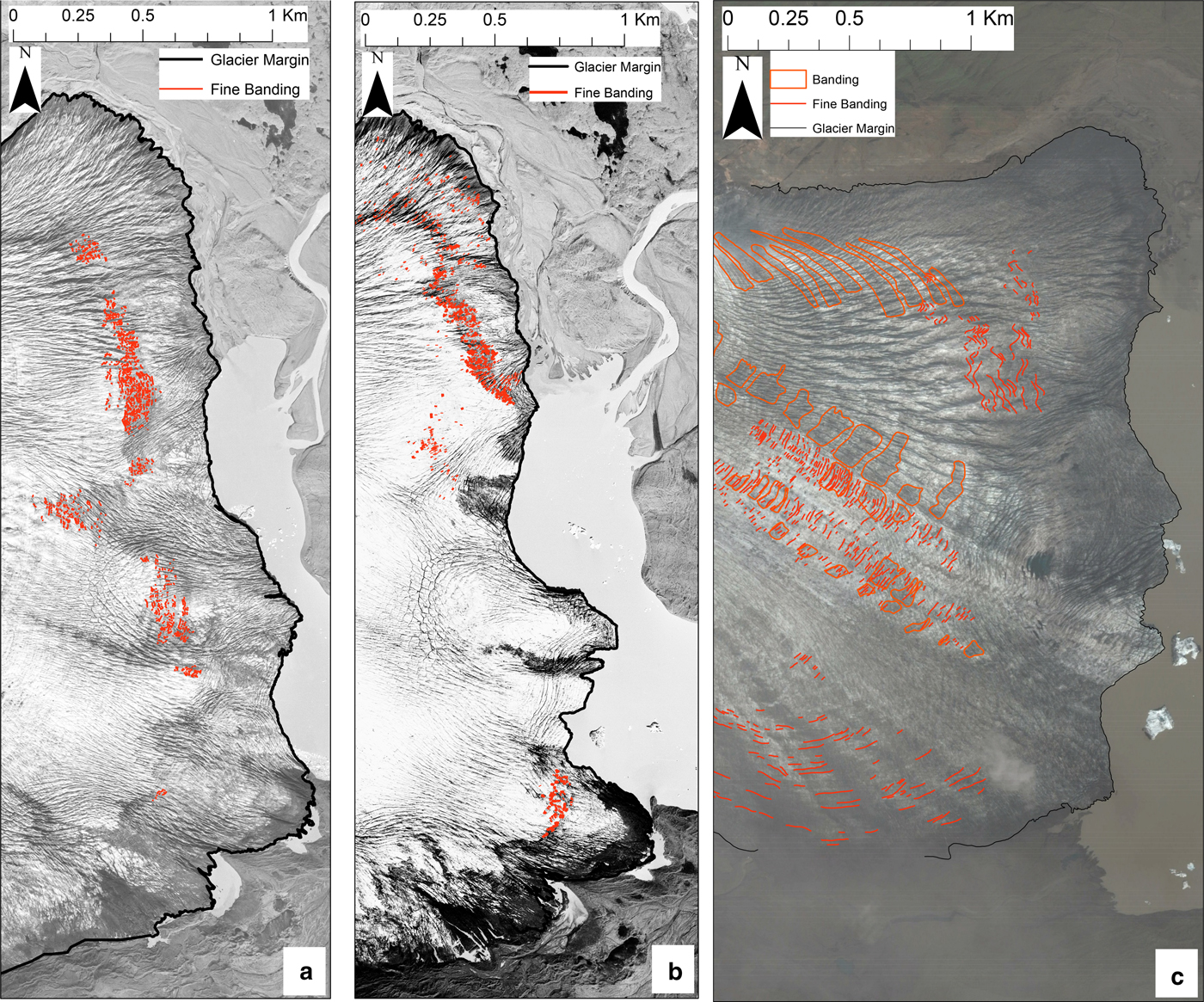
Fig. 8. Mapped ogive bands identified at Fjallsjökull's terminus in (a) 1982, (b) 1994 and (c) 2011.
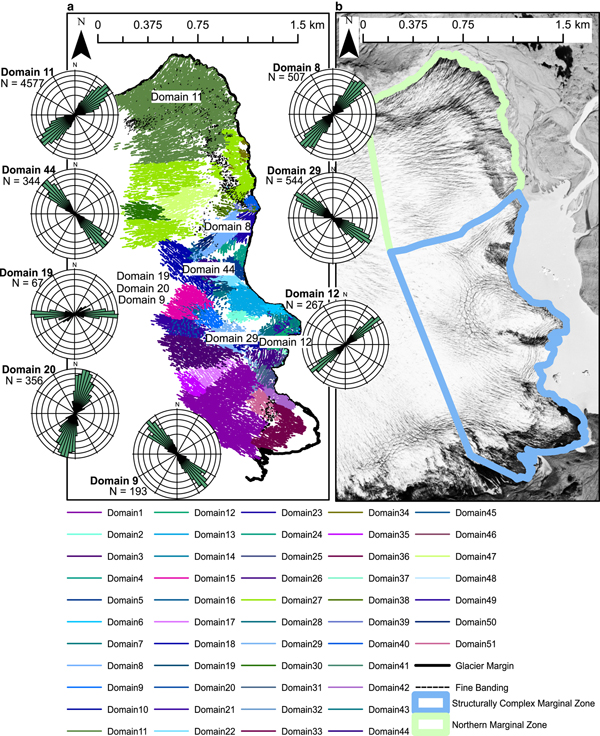
As in 1982, two key structural zones, the Northern Marginal Zone and the Structurally Complex Frontal Zone, were identified in the lower reaches of Fjallsjökull on the 1994 image (Fig. 9). The Northern Marginal Zone changed little since 1982, and its structure was characterised by a series of arcuate, closely spaced, open (~2–9 m wide) fractures (crevasses), arranged in a radial/splaying pattern (e.g. Domain 11) (Fig. 9). The spread in orientations for this zone was greater than in 1982, and fractures were orientated in a SW--NE to WSE--ENE direction (Fig. 9).
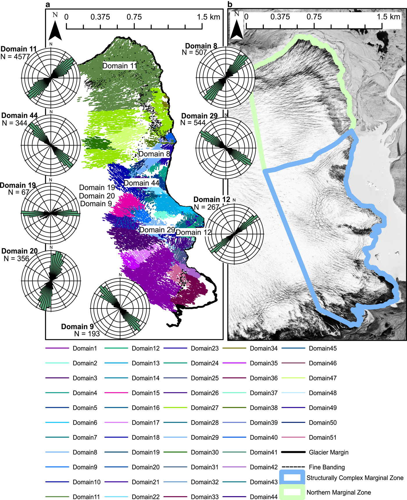
Fig. 9. (a) Mapped surface structures at Fjallsjökull's terminus in 1994, key domains are labelled and are also represented by rose diagrams, (b) The corresponding aerial photo, from which the surface structures were mapped (acquisition date: 9 August 1994, obtained from: The National Land Survey of Iceland (http://www.lmi.is/wp-content/uploads/2013/10/License-for-use-of-free-NLSI-data-General-Terms.pdf)). A fully labelled high-resolution version of this map can be found in the appendices (S.9).
In the Structurally Complex Frontal Zone in 1994, the surface fracturing was more complex than in 1982 (Fig. 9). This structurally complex zone was dissected by several sets of steeply dipping, straight, open (~1.5 to 10 m wide) fractures, which occurred approximately parallel to the calving front (e.g. Domain 12) (Fig. 9). These fractures cross-cut and offset a number of flow-parallel fracture sets, which are inferred to have formed in response to an earlier phase of deformation within the ice (Fig. 9). In addition, like in 1982, arcuate fracture patterns were also identified. One arcuate fracture pattern was positioned 500 m up-glacier of a prominent headland, and comprised a series of concave, down-ice dipping, open fractures belonging to four key Domains (Domains 9, 19, 20 and 29), which were arranged to form a distinct semi-circular geometry (Fig. 9). Similarly, a sweeping, arcuate fracture pattern, positioned 160 m up-glacier of a prominent embayment and formed by Domains 8 and 44 was also identified (Fig. 9). Fractures within both domains were straight to weakly curved, those belonging to Domain 8 trended in a SW--NE direction, whilst those belonging to Domain 44 trended in a NW--SE direction (Fig. 9).
Asymmetrical, weakly crenulated Ogive banding, with wavelengths of 20--50 m and amplitudes of 10--20 m was also identified in 1994 (Fig. 8b). This banding was predominantly identified towards the glacier's Northern Marginal Zone. However, within the Structurally Complex Frontal Zone this banding became largely overprinted or obscured as a result of locally intense brittle fracturing, although some small discrete patches of banding were still identified (Fig. 8b).
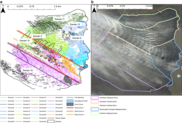
Detailed mapping of the 2011 imagery has enabled the lower reaches of Fjallsjökull to be divided into five key zones; (i) a Structurally Complex Frontal Zone, (ii) a Southern Marginal Zone, (iii) a Southern Central Zone, (iv) a Northern Central Zone and (v) the Northern Marginal Zone (Fig. 10).
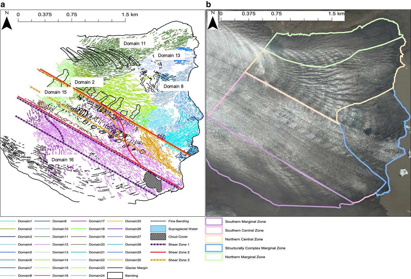
Fig. 10. (a) Mapped surface structures at Fjallsjökull's terminus in 2011, key domains are labelled and are also represented by rose diagrams, (b) The corresponding satellite image for the 29 June 2011, from which the surface structures were mapped (a Digital Globe Quick Bird image, downloaded via Google Earth). A fully labelled high-resolution version of this map can be found in the appendices (S.10).
The Northern Marginal Zone consisted of a single domain (Domain 11), this domain was characterised by a marked arcuate pattern of hook-shaped fractures, which curved towards the glacier margin, and trended from a SW--NE direction ~1.9 km up-glacier to a WSW--ENE direction closer to the glacier's terminus (Fig. 10). Overall, the Northern Marginal Zone changed little between 1982 and 2011 (Fig. 10). The Southern Marginal Zone identified in 2011 was also characterised by an arcuate pattern of approximately N--S trending, sub-vertical fractures (predominantly belonging to Domain 16), that curved towards the glacier margin (Fig. 10).
The Southern Central Zone was positioned between the Southern Marginal Zone and Northern Central Zone (Fig. 10). It comprised two main domains (Domains 12 and 15), which formed a sigmoidal to s-shaped pattern (Fig. 10). This geometry was consistent with fractures which formed as en-echelon tension fissures in response to brittle-ductile shearing of the ice (Fig. 10). These fracture sets defined a set of three prominent Y-type dextral strike-slip shear zones (Fig. 10). All three shear zones could be traced laterally for up to 2.5 km, and were in the order of 0.6 km wide (Fig. 10). The cross-cutting relationship between the individual domains within each shear zone enabled a relative chronology of shear zone formation to be established (Fig. 10). The relatively wide shear zone 1 formed first and was later cross-cut by the much narrower shear zone 2 (Fig. 10). Both shear zones 1 and 2 were cross-cut by the relatively younger shear zone 3, with the progressive narrowing of the shear zones possibly reflecting the greater partitioning of the brittle-ductile shear within the ice as deformation continued (Fig. 10). Furthermore, these cross-cutting relationships and narrowing of the shear zones suggests that over time there was a transition towards an increasingly concentrated flow regime along the glacier's central axis.
The Northern Central Zone was located immediately to the north of the Southern Central Zone and was characterised by a series of sweeping, arcuate fractures trending in a WSW--ENE direction with increasing proximity to the glacier's terminus (Fig. 10). The fractures within this zone were predominantly open (6 m wide), arcuate, and closely spaced (e.g. Domains 8 and 13) (Fig. 10). Between the glacier terminus and 1.4 km up-glacier, the boundary defining the Northern and Southern Central Zones was defined by a set of well-developed longitudinal fractures and strike-slip faults (Fig. 10). Further up-glacier, a set of open (2-7 m wide), semi-arcuate and sub-vertical fractures belonging to Domains 2 and 15 overprinted the fractures forming this boundary (Fig. 10). Both Domains were characterised by a series of sigmoidal to s-shaped fractures, defining a series of small shear zones, consistent with brittle-ductile shearing within the ice (Fig. 10). Domain 15 was situated up-glacier of Domain 2, and appears to have truncated the fractures identified within Domain 2 (Fig. 10).
The Structurally Complex Frontal Zone was characterised by cross-cutting relationships between the individual structural domains, accompanied by marked variation in fracture orientations. Adjacent domains were often composed of fracture sets orientated perpendicular to one another (Fig. 10). Overall, fractures within the Structurally Complex Frontal Zone were typically straight, steeply dipping and open.
In addition to the structures described above, Ogive banding was also prominent across Fjallsjökull in 2011. Each band was 1--10 m in width and composed of numerous short (50--100 m long) segments (Fig. 8c). The Ogive banding was characterised by marked spatial variations across the width of the terminus. The southern and northern marginal zones were characterised by simple, curved banding. Contrastingly, within the southern and northern central zones, the Ogive bands were dissected and modified by a combination of both brittle and ductile shear boundaries, leading to up to 53 m offset between banding sets (Figs 8c and 10). These shear boundaries were associated with changes in the glacier's flow regime, as the centre of the glacier transferred a pulse of fast flowing ice towards the frontal margin (Fig. 10).
4. DISCUSSION
4.1. Terminus position
Fjallsjökull's lake-terminating margin retreated by 1.21 km between 1973 and 2016 (Fig. 2) with the rate of retreat increasing significantly in 2001, 2009 and 2011 (Table 1). These findings are corroborated by earlier field observations in Hannesdóttir and others (Reference Hannesdóttir, Björnsson, Pálsson, Aðalgeirsdóttir and Guðmundsson2015) who measured the retreat of the margin between 1970 and 2010 at a single point on the land terminating section of the glacier. The greater retreat rates obtained during the present study (870 m of retreat in the period 1973--2010) compared to the study by Hannesdóttir and others (Reference Hannesdóttir, Björnsson, Pálsson, Aðalgeirsdóttir and Guðmundsson2015) (500 m of retreat between 1973 and 2010), can be partially explained by the differences between the methodologies used, but also by the fact that the lake-terminating portion of the margin is likely to retreat at a much faster rate than its land-terminating margin as a result of mass loss by calving in addition to surface ablation (Benn and others, Reference Benn, Warren and Mottram2007; Carrivick and Tweed, Reference Carrivick and Tweed2013).
The temporal pattern of terminus retreat at Fjallsjökull is also comparable to retreat patterns observed on many of Vatnajökull's outlet glaciers (e.g. Skalafellsjökull and Fláajökull) between ~1970 and 2010 (Schomacker, Reference Schomacker2010; Hannesdóttir and others, Reference Hannesdóttir, Björnsson, Pálsson, Aðalgeirsdóttir and Guðmundsson2015). In particular, the majority of Vatnajökull's outlet glaciers exhibited marked increases in their rate of retreat from ~1998 onwards (Hannesdóttir and others, Reference Hannesdóttir, Björnsson, Pálsson, Aðalgeirsdóttir and Guðmundsson2015). For example, between 1998 and 2010 and following a period of slow retreat, Skalafellsjökull and Fláajökull retreated by 350 and 538 m, respectively (Hannesdóttir and others, Reference Hannesdóttir, Björnsson, Pálsson, Aðalgeirsdóttir and Guðmundsson2015). The switch to increased retreat rates at Fjallsjökull, therefore, appears to be part of a wider regional trend.
4.2. Lake area change
Fjallsárlón increased by 2.72 km2 between 1973 and 2016, which was coincident with the continued development and expansion of other Icelandic proglacial lakes, particularly for outlet glaciers belonging to Vatnajökull (e.g. Breiðamerkurjökull, Svínafellsjökull, and Skaftafellsjökull) (Schomacker, Reference Schomacker2010). Furthermore, statistically significant increases in lake growth in 2001, 2009 and 2011 coincided with the statistically significant increases in terminus retreat rates for Fjallsjökull. A close correspondence between lake growth, accelerated retreat and increased flow velocities has also been observed at Breiðamerkurjökull (Storrar and others, Reference Storrar, Jones and Evans2017). Furthermore, at the same location, marked ice surface lowering and terminus retreat was observed (Storrar and others, Reference Storrar, Jones and Evans2017). Therefore, it appears that water depth exerts a key control on calving activity, surface lowering and acceleration of Breiðamerkurjökull (Storrar and others, Reference Storrar, Jones and Evans2017). Comparably, flow velocities at Fjallsjökull increased between 1999/2000 and 2014/15, with the greatest velocities corresponding to the deepest parts of the subglacial trench, where the lake depth is greatest.
Proglacial lake growth can initiate retreat through a number of processes. For example, it can lead to enhanced melt at the water line, enhanced melt below the waterline, and increased torque in response to an increase in buoyant forces (Benn and others, Reference Benn, Warren and Mottram2007; Dykes and others, Reference Dykes, Brook, Robertson and Fuller2011). These processes promote calving activity, and facilitate terminus retreat. Therefore, it is suggested that the observed co-incident increases in terminus retreat and lake expansion at Fjallsjökull are likely driven by processes such as torque and thermo-erosion as its proglacial lake expands. The portion of Fjallsjökull's terminus that was lake terminating increased by 40% between 1973 and 2016. This may have led to increased vulnerability of the terminus to calving events and, therefore, increased the rate of retreat.
4.3. Air temperatures: implications for thinning, terminus retreat and lake expansion
Our findings suggest that air temperatures may strongly influence the rates of surface elevation change, terminus retreat and lake expansion at Fjallsjökull (Figs 2, 3, and 4). Over the study period, mean annual air temperatures, mean summer surface air temperatures and PDD all rose by 2.1°C, 1.5°C and 511.3, respectively (Fig. 4). Furthermore, change-point analysis revealed statistically significant breaks in mean annual surface air temperatures in 1979 and 1992, in PDD in 1984 and 2001, and in mean summer surface air temperatures in 2015 (Table 1). The majority of these change points coincided with or briefly preceded statistically significant accelerations in the retreat rate and rate of lake area increase at Fjallsjökull, which occurred in 2001, 2009 and 2011 (Table 1). No clear relationship between precipitation and retreat rates was observed. However, this may be due to unreliable precipitation readings, resulting predominantly from wind induced undercatch (e.g. Yang and others, Reference Yang1999).
We suggest that the observed shifts to significantly warmer air temperatures in 1979 and 1992, and to significantly warmer summer air temperatures in 2015 may have led to increased thinning and ablation at Fjallsjökull. Available data show thinning rates of between c. −4 and −10 m for 2012/13 in crevasse free areas (Fig. 3). This thinning is likely to have contributed substantially to the expansion of Fjallsárlón as meltwater was ponded in the evolving proglacial lake basin. In addition, thinning may result in increased calving activity by (i) causing an increase in velocities, which results in longitudinal stretching and increased crevassing, and (ii) bringing the terminus nearer to flotation, which increases the potential for full thickness fracturing (Benn and others, Reference Benn, Warren and Mottram2007). Furthermore, when a terminus transitions towards floating conditions, it experiences a reduction in resistive stresses, and is therefore more susceptible to increased velocities and retreat rates (Joughin and others, Reference Joughin2008). In addition to rising air temperatures, a reduction in the albedo across Fjallsjökull, in response to a retreating snow line or darkening ablation zone, may have driven increased surface melt rates (Paul and others, Reference Paul, Machguth and Kääb2005).
Similarly to Fjallsjökull, dynamic responses to rising air temperatures and resultant glacier thinning have been previously observed across numerous glaciers elsewhere globally. For example, in Greenland, thinning of inland ice at Helheim led to a reduction in resistive forces and increased buoyancy of the terminus, which subsequently resulted in increased flow velocities and calving activity (Howat and others, Reference Howat, Joughin, Tulaczyk and Gogineni2005). Furthermore, at Tasman Glacier, a lake calving glacier in New Zealand, downwasting and thinning of the ablation zone has been observed throughout the 20th century, in line with climate warming. Between 1890 and 1986, some areas of the glacier thinned by 115--185 m (Dykes and others, Reference Dykes, Brook, Robertson and Fuller2011). Terminus retreat at Tasman Glacier then began in late 20th century; between 2000 and 2006, the average retreat rate was 54 m a−1 (Dykes and others, Reference Dykes, Brook, Robertson and Fuller2011). We suggest that similar processes and feedbacks are operating at Fjallsjökull, in line with rising atmospheric temperatures and resultant thinning.
Increased glacial retreat in response to atmospheric warming has also been seen at many other Icelandic outlet glaciers, including Sólheimajökull, Hyrningsjökull, Morsárjökull, Skaftafellsjökull (Sigurðsson and others, Reference Sigurðsson, Jónsson and Jóhannesson2007), and Kvíárjökull (Bennett and Evans, Reference Bennett and Evans2012). At Kvíárjökull, the area of the glacier snout decreased by more than 5% a−1 between 1998 and 2003, which coincided with a 0.45°C increase in average summer temperatures (Bennett and Evans, Reference Bennett and Evans2012). Furthermore, at Kvíárjökull, no correlation between precipitation and the rate of ice loss is found (Bennett and Evans, Reference Bennett and Evans2012). These observations, therefore, identify the significance of rising air temperatures for mass loss from Icelandic outlet glaciers. However, no studies have considered in detail the relationship between proglacial lake growth at Icelandic outlet glaciers and trends in air temperatures. Although, in the Himalaya (e.g. Gardelle and others, Reference Gardelle, Arnaud and Berthier2011; King and others, Reference King, Quincey, Carrivick and Rowan2016), and the Central Tibetan Plateau (Wang and others, Reference Wang, Siegert, Zhou and Franke2013), co-incident increases in proglacial lake size and air temperatures have been recorded. For example, in the Tibetan Plateau's Western Nyainqentanglha region, direct links between climate warming, glacier ablation and proglacial lake expansion have been made, with the region's glacier's reducing by 22% in aerial extent between 1977 and 2010, and the area of glacier lakes increasing by 173% between 1972 and 2009 (Wang and others, Reference Wang, Siegert, Zhou and Franke2013). We identify similar patterns at Fjallsárlón, as the lake extent increased by 303% in response to increasing air temperatures between 1973 and 2016.
4.4. Bed topography
Whilst the dynamic changes observed at Fjallsjökull were initiated by rising air temperatures, these changes were likely sustained and/or accelerated by local variations in the underlying bed topography. (Magnússon and others, Reference Magnússon, Pálsson, Björnsson and Guðmundsson2012) provide bed topography data for Fjallsjökull, which is predominantly based on points collected through a Radio Echo Sounding survey, conducted between 1998 and 2006. These data have an error of ±20 m in the z-axis (Magnússon and others, Reference Magnússon, Pálsson, Björnsson and Guðmundsson2012). Where data was sparse, they calculated pseudo profiles by estimating the relationship between the surface slope and the ice thickness (Magnússon and others, Reference Magnússon, Pálsson, Björnsson and Guðmundsson2012). These data were then interpolated to provide a contour map of Fjallsjökull (Fig. 11) (Magnússon and others, Reference Magnússon, Pálsson, Björnsson and Guðmundsson2012). Both Fjallsjökull and Fjallsárlón sit within a ~3 × 4 km subglacial trough, which lies up to 206 m below sea level (Fig. 11) (Magnússon and others, Reference Magnússon, Pálsson, Björnsson and Guðmundsson2012). Subglacial troughs exist beneath a number of outlet glaciers flowing from the Vatnajökull Ice Cap (e.g. Breiðamerkurjökull, Skaftafellsjökull, Svínafellsjökull), and often dam proglacial lakes as glaciers retreat (Schomacker, Reference Schomacker2010) (Fig. 1). As Fjallsjökull retreated across the depression, its proglacial lake was able to expand and likely deepen, facilitating further acceleration, thinning and retreat of the glacier into deeper water (Meier and Post, Reference Meier and Post1987; Vieli and others, Reference Vieli, Jania and Kolondra2002; Benn and others, Reference Benn, Warren and Mottram2007; Joughin and others, Reference Joughin2008; Carr and others, Reference Carr, Vieli and Stokes2013; Hill and others, Reference Hill, Carr, Stokes and Gudmundsson2018).
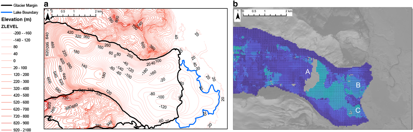
Fig. 11. (a) Bed topography dataset for Fjallsjökull displayed as a contour map with intervals of 20 m. (b) Calculated surface velocity data for Fjallsjökull in 2016/17, based on two Sentinel-2 MSI images. Labels A-C indicate notable features that reveal links between the surface velocities and bed topography data. ‘A’ indicates the origin of the faster flow, ‘B’ indicates the position of the northern fast flow ‘corridor’, and ‘C’ indicates the southern fast flow corridor, both ‘corridors’ align with a depression in the bed topography.
It is, therefore, likely that the increase in surface velocities at Fjallsjökull was in response to the expansion of Fjallsárlón, which resulted in increased calving activity and, as a result, increased ice draw down. We propose that the identified pulse of relatively fast flowing ice identified from the early 2000s onwards was initiated at region ‘A’, 4 km up-glacier of the terminus (Fig. 11). This region sits immediately down-ice of where the overdeepening begins, and is likely to have been the initial source of ice destabilisation in response to increased calving activity and ice draw down.
Secondly, two deeply incised channels exist within Fjallsjökull's bed topography, which currently underlie portions of the northern and southern portions of Fjallsjökull's terminus, and are likely to be controlling the location of the increasingly channelised flow (Fig. 11). The northern channel is elongate, and extends from 6.7 km up-glacier of the terminus position in 2011 towards the calving front, and reaches a maximum depth of 200 m below sea level (see ‘B’ in Fig. 11). The southern channel is 2 km × 2 km, and extends towards the calving front, reaching a maximum depth of 120 m below sea level (see ‘C’ in Fig. 11). These small-scale topographic variations likely influence local glacier dynamics, and in particular, the rate of retreat and glacier surface velocities. Where the glacier overlies localised deep channels, the rate of buoyancy driven calving may be greater, driven by processes such as torque due to buoyant forces (Benn and others, Reference Benn, Warren and Mottram2007). Furthermore, these two channels coincide with the two identified ‘fast flow corridors’, which develop at Fjallsjökull between 2014 and 2017 (Fig. 5). It is, therefore, likely that where the glacier overlies these relatively deep channels and experiences an increase in buoyancy driven calving, a positive feedback loop is initiated, facilitating further acceleration, draw down of up-glacier ice, thinning and further retreat (Meier and Post, Reference Meier and Post1987; Vieli and others, Reference Vieli, Jania and Kolondra2002; Benn and others, Reference Benn, Warren and Mottram2007; Joughin and others, Reference Joughin2008; Carr and others, Reference Carr, Vieli and Stokes2013; Hill and others, Reference Hill, Carr, Stokes and Gudmundsson2018).
At Breiðamerkurjökull, the large outlet glacier neighbouring Fjallsjökull, alterations in the glacier's dynamic regime have also been attributed to small-scale variations in the underlying topography (Storrar and others, Reference Storrar, Jones and Evans2017). Part of Breiðamerkurjökull terminates in a large proglacial lake, Jökulsárlón, and sits in an over-deepening that is up to 300 m below sea level (Björnsson, Reference Björnsson1996). Retreat rates and thinning rates are greatest here, where the glacier sits above a pronounced over-deepening (Nick and others, Reference Nick, Vieli, Howat and Joughin2009; Storrar and others, Reference Storrar, Jones and Evans2017). Evidence indicates that, like Fjallsjökull, the retreat of Breiðamerkurjökull over the Jökulsárlón trench drove a positive feedback loop, which led to increased rates of ice flow and ice surface draw down. This relationship was, again, predominantly attributed to the glacier's retreat into deeper water, which facilitated increased calving activity (Nick and others, Reference Nick, Vieli, Howat and Joughin2009; Storrar and others, Reference Storrar, Jones and Evans2017). We, therefore, infer that similar processes are operating at Fjallsjökull, and that retreat over the overdeepening encourages increased surface velocities and ice mass loss.
4.5. Concentrated flow at Fjallsjökull – a conceptual model
The proposed model combines the observed changes in surface velocities and surface structures to explain the development of a pulse of relatively ‘faster flow’ through distinct corridors, which conveyed ice to the calving front (Fig. 6). Three key stages have been identified: (1) Prior to 2000, a period of relatively slow flow (Fig. 5a) under a splaying flow regime. This is typical of ice spreading laterally to form a piedmont lobe as it leaves the confines of its valley (Fig. 6a); (2) a period between 2000 and 2015 in which there was the development of a pulse of relatively faster flow and the development of the northern ‘corridor’ (Figs 5c, 5d and 6b); and (3) the development of a secondary, southern fast flow ‘corridor’ between 2016 and 2018 (Figs 5e, 5f and 6c). The following interpretations are supported by detailed structural evidence, surface velocity fields, and bed topography data from Magnússon and others (Reference Magnússon, Pálsson, Björnsson and Guðmundsson2012). The detailed structural mapping method, first presented by Phillips and others (Reference Phillips2017) has recently undergone criticism for interpreting flow regimes with limited additional evidence (Swift and Jones, Reference Swift and Jones2018). However, the following sections of this paper provide interpretations of Fjallsjökull's flow regime, based on a combination of structural evidence, surface velocity fields and bed topography. This showcases the potential for detailed structural mapping to be incorporated into larger datasets for analysis of glacier flow and glacier modelling (Clarke and Hambrey, Reference Clarke and Hambrey2019).
4.5.1. Stage 1 (1990–2000)
This stage lasted from 1990 to 2000 (Figs 5a and 6a) and resulted in a radiating fan-like internal structural architecture to the glacier (Fig. 8) with relatively faster flow (~60–100 m a−1) along the centre line of the glacier and relatively slower flow at its margins (~20 m a−1) due to frictional drag along the valley walls. The structural architecture of the glacier shown on the 1994 structural map (Fig. 8) was consistent with the ice undergoing longitudinal compression and lateral extension as it flowed out of its confining valley (c.f. Colgan and others, Reference Colgan2016 and references therein). The observed structural regime at Fjallsjökull is expected for glaciers that terminate in a piedmont lobe (Post, Reference Post1972), as the margins are exposed to large transverse shear stresses, resulting in relatively slow flow at the glacier's margins (Lawson and others, Reference Lawson, Sharp and Hambrey1994). Similar splaying structures have previously been reported in Iceland (Phillips and others, Reference Phillips2017), New Zealand (Appleby and others, Reference Appleby, Brook, Vale and Macdonald-Creevey2010) and Alaska (Sharp and others, Reference Sharp, Lawson and Anderson1988).
4.5.2. Stage 2 (2000–15)
Stage two was characterised by increased surface velocities. Locally, the surface velocities at Fjallsjökull increased by ~30 m a−1 between 2000/01 and 2001/02 (Figs 5b and 5c), coinciding with a statistically significant change point in terminus retreat rates and lake expansion in 2001, in addition to an increase in the structural complexity of the glacier (Table 1). Furthermore, the increase in surface velocities followed identified change-points in atmospheric air temperatures (1979 and 1992) and in PDD (1984 and 2001) (Table 1). It can, therefore, be argued that this near-simultaneous acceleration in surface velocities, increase in terminus retreat rates and increase in lake expansion rates was predominantly driven by rising air temperatures and resultant thinning via surface ablation. Rising air temperatures likely led to persistent and widespread thinning of the terminus, which drove retreat of the glacier terminus, as the glacier became increasingly susceptible to full thickness fracturing (Benn and others, Reference Benn, Warren and Mottram2007). As the glacier terminus retreated into deeper water, a positive feedback loop likely resulted, further driving increased retreat rates and accelerated ice surface velocities (Benn and others, Reference Benn, Warren and Mottram2007). In 2014/15, a single, northern, ‘fast flow’ corridor extended from 4 km up-glacier, towards the calving front (see region D in Fig. 5d).
The observed velocity changes between 2000 and 2015 are also detected by the structural results. The increasingly channelised faster flow over this period corresponded to an increase in the structural complexity of the glacier and the forward movement of ice within the corridor, which resulted in shearing at its margins. These shear margins were marked by dextral strike-slip faults (as identified in the 2011 structural map), where Domain 15 locally overprinted Domain 2, ~1.4 km up-glacier of the calving front (Fig. 9). The ice within this corridor was also heavily crenulated, with banding exhibiting amplitudes of between 5 and 30 m, indicating marked lateral compression of the ice within this region. Furthermore, the surface velocity results identified the source of this relatively faster flowing pulse of ice to have originated from region ‘A’, not from the accumulation zone on Öræfajökull. The destabilisation of ice in region ‘B’ may have occurred above the up ice boundary of the overdeepening, as ice draw down was initiated in response to increased calving activity as the proglacial lake expanded (Fig. 5). Furthermore, a series of three dextral strike-slip shear zones are apparent in the 2011 structural assessment towards the south of Fjallsjökull's terminus (Fig. 9). The cross-cutting relationships between the fracture sets in this zone reflected the narrowing of dextral strike-slip shear zones over time (Fig. 10). These shear zones have likely formed in response to the gradual narrowing of a zone of faster surface velocities in the south of Fjallsjökull's terminus since the year 2000, as region ‘C’ begins to dimish in area, whilst flow velocities continue to increase (Figs 5b, 5c and 5d).
Overall, an increase in the calving rate of a glacier, such as Fjallsjökull, may result in the development of a positive feedback loop, as an increase in calving increases the net drawdown of ice through the glacier's system, steepening the glacier's surface, and further facilitating an increase in mass loss as the glacier retreats into deeper water (Carrivick and Tweed, Reference Carrivick and Tweed2013). A similar scenario has been previously observed at Mendenhall Glacier, south-east Alaska; the glacier thinned and retreated into deeper water until it reached flotation and destabilised (Motyka and others, Reference Motyka, O'Neel, Connor and Echelmeyer2003). Once destabilised, the glacier terminus began to calve at an increased rate into its proglacial lake, which was related to retreat into deeper water and initiated a positive feedback loop (Motyka and others, Reference Motyka, O'Neel, Connor and Echelmeyer2003).
4.5.3. Stage 3 (2016–18)
By 2016, an additional, southern ‘fast flow’ corridor had fully developed at Fjallsjökull (see region ‘E’ in Figs 5e and 5f). It is likely that the spatial arrangement of Fjallsjökull's flow regime was primarily influenced by the underlying bed topography (Fig. 11) (Magnússon and others, Reference Magnússon, Pálsson, Björnsson and Guðmundsson2012). This may have increasingly impacted surface ice velocities as the glacier retreated back into its over-deepening, and as it thinned under rising air temperatures. The two identified ‘fast flow’ corridors at Fjallsjökull were underlain by prominent depressions in the bed topography (Fig. 11) (Magnússon and others, Reference Magnússon, Pálsson, Björnsson and Guðmundsson2012). Where the glacier retreated across these depressions, processes including buoyancy driven calving, torque due to buoyant forces and thermally induced melt increased where the glacier entered deeper water (Benn and others, Reference Benn, Warren and Mottram2007; Nick and others, Reference Nick, Vieli, Howat and Joughin2009; Porter and others, Reference Porter2014; Carr and others, Reference Carr2015). The spatial signature of velocity changes at Fjallsjökull, therefore, suggest that the observed increases in velocities resulted from retreat rather than increased basal lubrication. This argument is supported by the work of Tedstone and others (Reference Tedstone2015), who suggest that hydrodynamic coupling at the ice bed interface may reduce net ice surface velocities, as increased meltwater input to the ice bed interface results in the development of an increasingly channelised drainage system, which exports water delivered to the ice/bed interface before it can act as a basal lubricant.
5. CONCLUSIONS
Overall, this study highlights the significance of glacier specific (e.g. bed topography) and non-glacier specific (e.g. climate) controls on the dynamic and structural regime of Fjallsjökull. The combination of the structural and velocity data has provided a greater insight into the spatial complexities of the glacier's evolution. We identified statistically significant change-points for both terminus position and lake area change in 2001, 2009 and 2011. The synchronous increased rates of terminus retreat and lake expansion reveals a link between the two processes, which we propose is driven by an increase in longitudinal stresses acting on the glacier terminus as the proglacial lake extent increases. We identify rising atmospheric air temperatures as a key control on terminus position and lake area at Fjallsjökull. Our conceptual model, which combines an assessment of changes to the glacier's surface velocities and structural architecture over the study period, reveals the development of an increasingly spatially complex flow regime over time, characterised by a series of ‘fast flow’ corridors. Dextral-strike slip faults facilitate this flow regime, as they allow corridors of faster flowing ice to propagate towards the terminus. Furthermore, we argue that the spatial complexities of the concentrated flow regime are governed by the bed topography that underlays the glacier. The influence of this bed topography on the glacier's dynamic and structural regime appears to have increased throughout the study period, as the glacier has thinned due to rising atmospheric air temperatures.
SUPPLEMENTARY MATERIAL
The supplementary material for this article can be found at https://doi.org/10.1017/jog.2019.18.
ACKNOWLEDGMENTS
We would like to thank Eyjólfur Magnússon for sharing with us his bedrock topography data for Fjallsjökull. Furthermore, we are very grateful to our reviewers, Anders Schomacker and Rob Storrar, for providing positive and constructive feedback during the review process. Rebecca acknowledges support from a masters scholarship, provided by the school of Geography, Politics, and Sociology, Newcastle University and support from a Natural Environment Research Council Doctoral Training Partnership Studentship (Grant number: NE/L002507/1).


 Open access