


1. Introduction
Mountain glaciers comprise 1% of global glacier ice volume yet account for ∼1/3 of modern global sea level rise (Hugonnet, Reference Hugonnet2021). Of these glaciers, those that terminate in water show the largest changes in response to global warming, often due to abrupt collapses of the glacier tongue (Truffer and Motyka, Reference Truffer and Motyka2016). Ongoing global glacier retreat has led to an increase in the number and size of proglacial lakes (Zhang, Reference Zhang2024), here defined as freshwater lakes in direct contact with ice at the glacier terminus. Glaciers that terminate in the ocean (marine-terminating glaciers) are known to undergo rapid and irreversible retreat (Pfeffer, Reference Pfeffer2007), raising concern about the dynamical stability of lake-terminating glaciers (Carrivick and Tweed, Reference Carrivick and Tweed2013). Lake-terminating-glaciers have been observed to flow faster (Pronk and others, Reference Pronk, Bolch, King, Wouters and Benn2021; Main, Reference Main2023) and thin more rapidly than land-terminating glaciers (Larsen and others, Reference Larsen2015; King and others, Reference King, Bhattacharya, Bhambri and Bolch2019; Minowa and others, Reference Minowa, Schaefer, Sugiyama, Sakakibara and Skvarca2021), which is often interpreted to reflect the lakes driving enhanced velocity or mass loss. However, lake-terminating glaciers are thought to respond less sensitively due to the presence of water at their termini than marine-terminating glaciers (Benn and others, Reference Benn, Warren and Mottram2007a; Minowa and others, Reference Minowa, Schaefer and Skvarca2023) because the rate of frontal ablation, the sum of subaqueous melt and calving at the glacier terminus are is expected to be lower in lacustrine settings (Truffer and Motyka, Reference Truffer and Motyka2016). In marine environments, iceberg calving is enhanced in deeper waters where ice is more likely to float and fracture along planes of weakness (Brown and others, Reference Brown, Meier and Post1982; Benn and others, Reference Benn, Warren and Mottram2007a; Nick and others, Reference Nick, Veen, Vieli and Benn2010). Subaqueous melt in marine settings is often driven by buoyant subglacial meltwater discharge entraining warm ambient fjord water, with the potential for rapid melt due to water’s high heat capacity and heat transfer coefficient (Truffer and Motyka, Reference Truffer and Motyka2016). High rates of subaqueous melt may further enhance calving by undercutting the terminus. Thus, the lack of buoyancy-driven melt enhancement and replenishment of warm subsurface waters in lacustrine settings (Truffer and Motyka, Reference Truffer and Motyka2016; Sugiyama and others, Reference Sugiyama, Minowa and Schaefer2019) may result in far lower rates of frontal ablation for lake-terminating glaciers than their marine counterparts (Trüssel and others, Reference Trüssel, Truffer, Hock, Motyka, Huss and Zhang2015). However, lake-terminating glaciers more frequently exhibit persistent floating tongues, buoyancy-driven calving (Boyce and others, Reference Boyce, Motyka and Truffer2007; Trüssel and others, Reference Trüssel, Truffer, Hock, Motyka, Huss and Zhang2015; Minowa and others, Reference Minowa, Schaefer and Skvarca2023) and terminus ‘over-cutting’ leading to underwater ice terraces (Robertson and others, Reference Robertson, Benn, Brook, Fuller Lan and Holt2012; Sugiyama and others, Reference Sugiyama, Minowa and Schaefer2019), which may make their dominant frontal ablation processes somewhat dissimilar from temperate marine-terminating glaciers.
Frontal ablation is a substantial contributor to mass loss for marine-terminating glaciers across the world (Mouginot, Reference Mouginot2019; Rignot and others, Reference Rignot2019; Kochtitzky, Reference Kochtitzky2022), but the contribution of frontal ablation to the mass loss of the world’s lake-terminating glaciers is largely unknown. In the only known regional study addressing lake-terminating glacier frontal ablation, the median contribution of frontal ablation to mass loss across 30 Patagonian lake-terminating glaciers was estimated to be 13%, with the proportion reaching 50% on some glaciers (Minowa and others, Reference Minowa, Schaefer, Sugiyama, Sakakibara and Skvarca2021). On a rapidly retreating Alaska lake-terminating glacier, frontal ablation was estimated to account for 8–17% of mass loss (Trüssel and others, Reference Trüssel, Truffer, Hock, Motyka, Huss and Zhang2015). Despite the potential for a mechanism for additional mass loss, no regional estimate exists to constrain the magnitude of frontal ablation on Alaska’s lake-terminating glaciers, nor its potential impact on glacier change.
Ice-marginal lakes (i.e. either proglacial, ice-dammed or supraglacial) expanded rapidly in recent decades, with an increase in both number and areal extent of lakes documented from Patagonia (Wilson, Reference Wilson2018) to Greenland (How, Reference How2021) and many areas in between (e.g. Chen, Reference Chen2021; Mölg, Reference Mölg2021; Carrivick, Reference Carrivick2022). Over 14 400 ice-marginal lakes now exist across the world, covering an area of 9000 km2 with a volume of 157 km3 (Shugar, Reference Shugar2020). In Alaska, ice-marginal lakes grew approximately three times faster than the global average, with proglacial lakes increasing in area by 85% between 1984 and 2019 to now cover 1000 km2 (Rick and others, Reference Rick, McGrath, Armstrong and McCoy2022). The formation and drainage of proglacial lakes can have profound effects on the surrounding environment and downstream communities by altering suspended sediment flux and stream flow characteristics, creating habitats (Dorava and Milner, Reference Dorava and Milner2000), changing downstream water resources (Farinotti and others, Reference Farinotti, Round, Huss, Compagno and Zekollari2019) and increasing risk of glacial lake outburst floods when a lake dam fails or is overtopped (Carrivick and Tweed, Reference Carrivick and Tweed2013; Rick and others, Reference Rick, McGrath, Armstrong and McCoy2022; Veh and others, Reference Veh, Lützow, Tamm, Luna, Hugonnet, Vogel, Geertsema, Clague and Korup2023). Proglacial lake growth should also influence the rates of frontal ablation, as larger lakes have more surface area available to absorb solar radiation, resulting in warmer water temperatures and higher rates of subaqueous melt (Trüssel and others, Reference Trüssel, Truffer, Hock, Motyka, Huss and Zhang2015; Sugiyama, Reference Sugiyama2016). Larger lakes also tend to be deeper (Cook and Quincey, Reference Cook and Quincey2015), so lake growth may result in higher flotation fractions and more vigorous mass loss through calving.
This study provides new insight into freshwater frontal ablation processes by quantifying the retreat rates of Alaska’s lake-terminating glaciers since 1984 using Landsat imagery and comparing retreat values with those found on Alaska marine-terminating glaciers (McNabb and others, Reference McNabb, Hock and Huss2015). Combining new satellite-derived terminus position observations and previously published geospatial datasets (i.e. ice thickness and velocity), we use a mass conservation approach to estimate the rates of frontal ablation on Alaska’s lake-terminating glaciers. We then explore associations between environmental variables (e.g. lake area, glacier area, estimated flotation fraction) and the observed retreat and frontal ablation rates. Lastly, we use existing geospatial datasets to estimate the time remaining for lake-terminating glaciers to retreat above the recent lake surface elevation, providing an estimate for when these glaciers will become land-terminating.
2. Methods
2.1. Study area
Our study focuses on Alaska and northwest Canada, a region where ice-marginal lakes grew three times faster than the global average between 1990 and 2018 (Shugar, Reference Shugar2020). The region’s proglacial lakes grew faster than other types of ice-marginal lakes (e.g. ice-dammed or supraglacial lakes), increasing in area by 85% (543–1006 km2) between 1984 and 2019 (Rick and others, Reference Rick, McGrath, Armstrong and McCoy2022). This rapid expansion of proglacial lakes coincides with accelerated loss of glacial ice in the Alaska-British Columbia-Yukon region (Randolph Glacier Inventory, RGI, Region 01), which had a mean surface lowering rate of 0.91 m a−1 between 2000 and 2019 (Hugonnet, Reference Hugonnet2021). The region’s abundance of rapidly changing proglacial lakes makes it an ideal site to capture the range of behavior possible on lake-terminating glaciers.
Our study focuses on 55 lake-terminating glaciers covering ∼14 000 km2 and spanning 56–64° N and 130–154° W (Fig. 1). This dataset includes most of the lake-terminating glaciers in RGI Region 01 >100 km2, as well as the region’s 14 most rapidly growing proglacial lakes that formed during the Landsat record (Rick and others, Reference Rick, McGrath, Armstrong and McCoy2022), 8 of which are <100 km2. We exclude several glaciers that the RGI defines as lake-terminating (RGI Region 01 IDs: 12425—Triumvirate Glacier, 17348—Russell Glacier, 20796—Brady Glacier) because they lack true proglacial lakes. In these cases, ice-dammed or small proglacial lakes are found near the terminus, but the glaciers lack a large, coalesced lake downstream from the terminus. Our study glaciers cover 83% of all lake-terminating glacier area in RGI region 01 as defined by the RGI Version 6 (Figure S1). We focus on the larger lake-terminating glaciers from the RGI to facilitate higher quality ice thickness and velocity data. By adding the 14 fastest-growing new proglacial lakes from Rick and others (Reference Rick, McGrath, Armstrong and McCoy2022), we seek to provide an upper bound on lake-terminating glacier retreat and presumably frontal ablation rates.
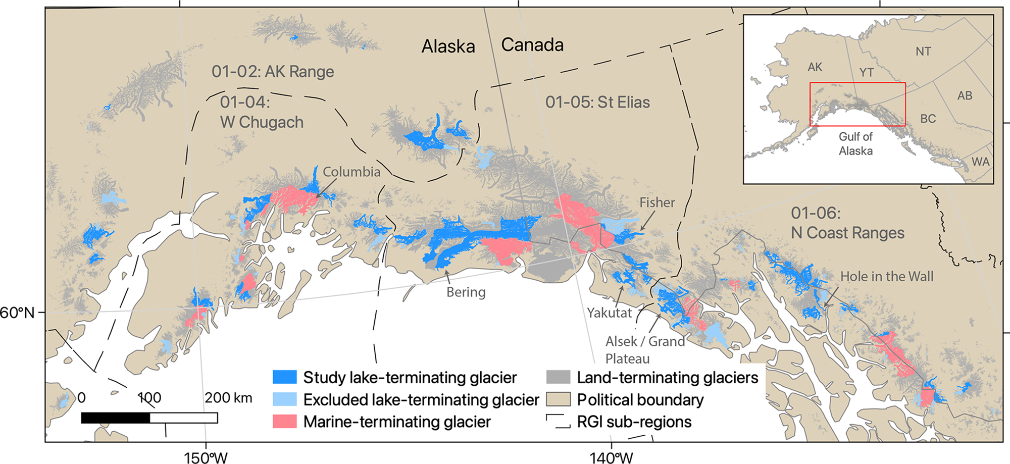
Figure 1. Distribution of study glaciers in Alaska and northwest Canada used for this research. Lake-terminating glaciers considered in this study (n = 55) are shown in dark blue stars, with marine-terminating glaciers (n = 27) from McNabb and others (Reference McNabb, Hock and Huss2015) shown in pink. Light blue glaciers are classified as lake-terminating by the Randolph Glacier Inventory (RGI) v6 but were excluded from this study either due to the 100 km2 glacier area minimum threshold or special circumstances described in the text. RGI region 01 subregions are delineated by black lines and labeled with gray text. Some minor discrepancies exist between the glacier outlines of McNabb and others (Reference McNabb, Hock and Huss2015) and those shown here, which are from RGI Consortium (2017). Map is projected in Alaska Albers (EPSG:3338).
2.2. Quantifying glacier retreat rates
We use the Google Earth Engine Digitisation Tool (GEEDiT; Lea, Reference Lea2018) to manually digitize glacier terminus positions with annual resolution from primarily melt season (May–September) Landsat imagery spanning 1984–2021. Length change time series are calculated using the single central flowline method provided by the Margin Change Quantification Tool (MaQIT; Fig. 2; Lea, Reference Lea2018). We use the centerlines provided by the Open Global Glacier Model (Maussion, Reference Maussion2019; accessible at https://docs.oggm.org/en/stable/assets.html).
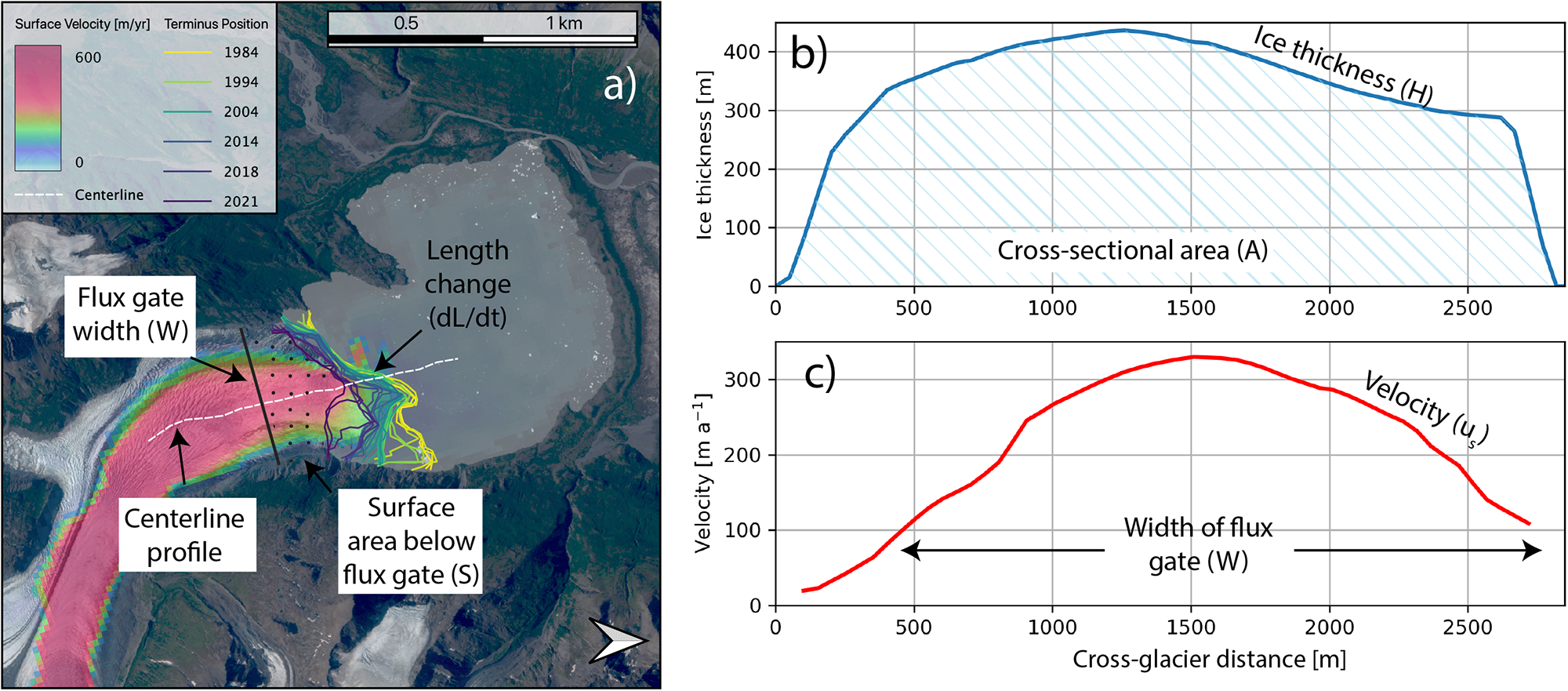
Figure 2. Physical overview of quantities used to estimate retreat and frontal ablation rates. (a) Surface velocity map of Colony Glacier (RGI60-01.10006). Digitized glacier terminus positions, measured annually using GEEDiT (Lea, Reference Lea2018), are shown as lines with a gradient color scheme. The near terminus flux gate, set upstream of the furthest upstream terminus position, is used to calculate ice flux in and out of the near-terminus control volume. The surface area below cross section (S) is used to calculate mass loss from surface melt. (b) Ice thickness (line) and cross-sectional area (hatched area) used to calculate mass flux across flux gate with the addition of (c) ice surface velocity and width of flux gate. Ice thickness and surface velocity data are from Millan and others (Reference Millan, Mouginot, Rabatel and Morlighem2022). Background image in (a) is a 2018 Sentinel-2 image.
We assess temporal variations in retreat rate by calculating the average rate of length change over the entire study period as well as three approximately decadal periods: 1986–98, 1999–2008 and 2009–18. These time periods align with the lake area delineations of Rick and others (Reference Rick, McGrath, Armstrong and McCoy2022), which allows us to investigate possible relationships between proglacial lake area and glacier retreat rate. For each glacier, we isolated length data in each period. Within that period, we obtained a linear fit to the data using the nonparametric Theil–Sen regression method (Helsel and others, Reference Helsel, Hirsch, Ryberg, Archfield and Gilroy2020). Given the sparse number of observations for each time period, we used the Theil–Sen regression method because it is resistant to outliers and does not assume input data are normally distributed. The slope of the Theil–Sen fit line provides our estimate of average rate of length change during the period. While ordinary least squares regression would likely produce similar results for this analysis of changes in retreat rates, we employ Theil–Sen correlation here for methodological consistency with for our later analyses (Section 2.6) in which outlying data points would skew the overall statistical results provided by ordinary least squares.
There is short-term variability in retreat rates due to image timing and seasonality of retreat, but, as our study is focused on multi-decadal behavior, we neglect seasonal variations in retreat and frontal ablation. The middle 80% (10th–90th percentiles) of our input imagery comes from days of year (DOYs) 132–274 (11 May–30 September), with a median image DOY of 198 (16 July; Fig. S2).
2.3. Estimating rates of frontal ablation
Following the approach of McNabb and others (Reference McNabb, Hock and Huss2015), we estimate frontal ablation rates by first defining mass conservation below a near-terminus flux gate, given as:
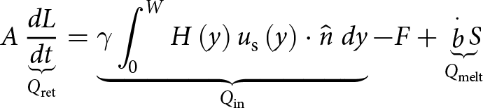 \begin{equation}A\underbrace {\frac{{dL}}{{dt}}}_{{Q_{\text{ret}}}} = \underbrace {\gamma \int_0^W {H\left( y \right){u_{\text{s}}}\left( y \right) \cdot \widehat n\;dy}}_{{Q_{\text{in}}}} - F + \underbrace {\mathop b\limits^. S}_{Q_{\text{melt}}} \end{equation}
 where A is the cross-sectional area of the near-terminus flux gate estimated from the Millan and others (Reference Millan, Mouginot, Rabatel and Morlighem2022) modeled ice thickness estimates,  $\frac{{dL}}{{dt}}$ is the Theil–Sen slope-estimated retreat rate, $\gamma $ is a parameter that scales the surface velocity to column-averaged velocity and H and u s are respectively modeled ice thickness and remotely sensed ice surface velocity from Millan and others (Reference Millan, Mouginot, Rabatel and Morlighem2022). W is glacier width, y is the flow-transverse coordinate, $\hat n$ is the vector normal to the flux gate, F is the frontal ablation rate, $\dot b$ is the assumed surface mass balance and S is the glacier’s surface area between the flux gate and terminus (Fig. 2a). Flux gate locations were chosen to be as close to the modern terminus position as possible while maintaining physically plausible surface velocity and ice thickness data, which often decline in quality toward the terminus. Conceptually, the left-hand side of Eqn (1) represents mass change in the ‘control volume’ below the flux gate due to advance or retreat (Q ret), which is set by the balance of mass gain due to ice flow across the flux gate (first term on right-hand side; Q in) and mass loss through frontal ablation (F) and surface melt (the third terms on right-hand side; Q melt). Basal velocities are generally high near calving fronts (Cuffey and Paterson, Reference Cuffey and Paterson2010) and we set $\gamma = 0.9$ reflecting roughly equal contributions of basal motion and internal deformation to glacier surface velocity. Following McNabb and others (Reference McNabb, Hock and Huss2015), we assume a high estimate of −10 m a−1 for surface mass balance ( $\dot b$), which matches the most negative surface mass balance value found near the terminus of a single marine-terminating glacier (Columbia Glacier; Rasmussen and others, Reference Rasmussen, Conway, Krimmel and Hock2011). We stress that this assumed value of $\dot b$ is not applied over the glacier’s entire area but only applied over the relatively small surface area below the flux gate (S; Fig. 2a). Using a high estimate of surface mass balance and an intermediate value for $\gamma $ yields conservative (i.e. low) estimates of frontal ablation and is consistent with the methodology of McNabb and others (Reference McNabb, Hock and Huss2015), facilitating direct comparison of our estimates. We note that, by convention, negative $\frac{{dL}}{{dt}}$ indicates glacier retreat, positive Q in indicates mass gain, positive F represents mass loss through frontal ablation and $\dot b$ corresponds to surface melt. Rearranging (1) to solve for frontal ablation (F), we have:
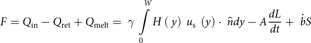 \begin{equation}F = {Q_{\text{in}}} - {Q_{\text{ret}}} + {Q_{\text{melt}}} = {\text{ }}\gamma {\text{ }}\mathop \int \limits_0^W H\left( {{\text{ }}y} \right){\text{ }}{u_{\text{s}}}{\text{ }}\left( y \right) \cdot {\text{ }}\hat ndy - A\frac{{dL}}{{dt}} + {\text{ }}\dot bS\end{equation}
where all terms have been defined previously (Table S1).
Unless otherwise stated, all estimate of frontal ablation below use  $\frac{{dL}}{{dt}}$ from 2009–18, as it is the study subperiod that best aligns with the timing of the other input datasets. Surface velocities ( ${u_{\text{s}}}$) in Millan and others (Reference Millan, Mouginot, Rabatel and Morlighem2022) reflect an average over 2017–18, and associated thickness is estimated using a multitemporal DEM built from stereo imagery collected from ASTER (launched in 1999) and the WorldView constellation (first launched in 2007), with results computed over an average ∼2010 glacier outline (RGI Consortium, 2017). Utilizing the slower average $\frac{{dL}}{{dt}}$ rates estimated over the whole 1984–2021 study period results in a median decrease in F of 0.001 Gt a−1, with an interdecile range of −0.021 to 0.071 Gt a−1 (negative values indicate lower F using the 2009–18 retreat rates, which would be produced by retreat rate slowing over time; Fig. S3).
2.4. Estimating uncertainty in frontal ablation
To estimate errors, we simplify Eqn (2) into a cross-sectionally averaged form,
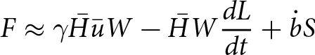 \begin{equation}F \approx \gamma \bar H\bar uW - \bar HW\frac{{dL}}{{dt}} + \dot bS\end{equation}
 where overbars indicate the average value across the cross-section. We estimate uncertainty in the first two terms, which respectively represent mass gained from ice flux across the flux gate (Q in) and mass lost through terminus retreat (Q ret), as described below. We assess the uncertainty of our estimates of F due to the assumed high-end plausible mass balance value ( $\mathop b\limits^. $ = −10 m a−1) by recalculating F with $\mathop b\limits^. $ = −5 m a−1 and find a median F increase of 0.006 Gt a−1 (9%; Fig. S4). Importantly, a lower near-terminal surface melt rate results in higher estimated frontal ablation rates, so our results present a conservative (i.e. low) figure (described further in Section 2.3). The actual uncertainty due to the assumed surface mass balance below the flux gate is a systematic error of unknown magnitude, which we omit from the following error propagation, but the analysis above gives an idea of its relative magnitude.
Assuming error terms are independent and normally distributed, uncertainty in the incoming ice flux ( $\delta {Q_{\text{in}}}$) is given as
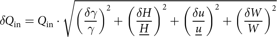 \begin{equation}\delta {Q_{\text{in}}} = {Q_{\text{in}}} \cdot \sqrt {{{\left( {\frac{{\delta \gamma }}{\gamma }} \right)}^2} + {{\left( {\frac{{\delta H}}{{\underline{H} }}} \right)}^2} + {{\left( {\frac{{\delta u}}{{\underline{u} }}} \right)}^2} + {{\left( {\frac{{\delta W}}{W}} \right)}^2}} \end{equation}
 where we use  $\delta \gamma = 0.1$ and $\delta W = 60$ m (±1 pixel) as set values, with the remaining terms varying on a glacier-by-glacier basis. For $\delta H$ and $\delta u$, we take the mean stated uncertainty (Millan and others, Reference Millan, Mouginot, Rabatel and Morlighem2022) across the cross-section. In general, the ice thickness dataset differs from measurements within ±25% for ice thicker than 200 m (Figs S3 and S9 in Millan and others, Reference Millan, Mouginot, Rabatel and Morlighem2022). Radar observations for ground-truthing these estimates across Alaska remain sparse (Welty, Reference Welty2020; Tober, Reference Tober2023), but for the median flux gate ice thickness of 403 m across our study glaciers, the ±25% corresponds to ∼±100 m (Millan and others, Reference Millan, Mouginot, Rabatel and Morlighem2022). Utilizing velocity data from 2017–18 to compute frontal ablation rates over 2009–18 relies on an implicit assumption that annual average velocity does not vary significantly over the longer time period. This assumption results in additional uncertainty in Q in that cannot be estimated without outside knowledge of how representative the 2017–18 velocity is for the 2009–18 period, as well as how this varies across glaciers. We acknowledge this limitation but still utilize the dataset due to its widespread geographic coverage, well-quantified error and ease of use. Ice thickness also represents a 2017–18 snapshot in time, but systematic changes in ice thickness over 2009–18 are likely small relative to the random error in the Millan and others (Reference Millan, Mouginot, Rabatel and Morlighem2022) ice thickness described above.
Uncertainty in Q ret is calculated in a similar manner to that for  ${Q_{\text{in}}}$and we then estimate uncertainty in frontal ablation ( $\delta F$) as
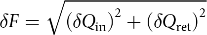 \begin{equation}\delta F = \sqrt {{{\left( {\delta {Q_{\text{in}}}} \right)}^2} + {{\left( {\delta {Q_{\text{ret}}}} \right)}^2}} \end{equation}
 On average,  $\delta {Q_{\text{in}}}$ is 28% of ${Q_{\text{in}}}$ and $\delta {Q_{\text{ret}}}$ is 26% of ${Q_{\text{ret}}}$. Uncertainty is estimated in frontal ablation scales with the magnitude of frontal ablation, with an average of 24% (Fig. S5).
2.5. Comparison marine-terminating glacier data set
We compare our estimated rates of retreat and frontal ablation for lake-terminating glaciers with estimates for Alaska’s marine-terminating glaciers from McNabb and others (Reference McNabb, Hock and Huss2015). The McNabb dataset consists of 27 marine-terminating glaciers covering an area of ∼11 000 km2 (Fig. 1), while the 55 lake-terminating glaciers in this study cover ∼14 000 km2. These marine-terminating glaciers represent 96% of the total tidewater glacier area in Alaska, accounting for 12.6% of the total RGI Region 1 glacier area (McNabb and others, Reference McNabb, Hock and Huss2015). The marine-terminating dataset incorporates Landsat data spanning 1985–2013 with at least five observations of terminus positions per year on average and reported average uncertainties in retreat and frontal ablation of 10% and 24%, respectively.
2.6. Investigating potential physical drivers and forecasting long-term change
We manually identified the lake surface elevation and extracted glacier centerline surface elevation (Z s) profiles using the Copernicus 3 arc-second (GLO-90; ∼90 m pixel) digital elevation model (European Space Agency, 2024). We utilize this dataset rather than a higher resolution time-stamped source like the ArcticDEM because lake elevation is often poorly resolved in this optical image-derived dataset, file sizes are large enough that data analysis becomes more cumbersome, and our analysis does not require fine spatial resolution. The GLO-90 DEM represents the land surface over 2011–15 and covers the high latitudes with <4 m elevation uncertainty (European Space Agency, 2024). The dataset’s survey date roughly corresponds with the modal 2010 glacier outline date for the RGI in this region (RGI Consortium, 2017), which is an input to the Millan and others (Reference Millan, Mouginot, Rabatel and Morlighem2022) ice thickness dataset. We then estimated the glacier bed elevation (Z b; Fig. 3) by subtracting the Millan and others (Reference Millan, Mouginot, Rabatel and Morlighem2022) ice thickness from the GLO-90 surface elevation along the glacier centerline using profiles from Maussion (Reference Maussion2019) as,
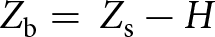 \begin{equation}{\text{ }}{Z_{\text{b}}} = {\text{ }}{Z_{\text{s}}} - H\end{equation}
Figure 3. Surface (red) and bed elevation (blue) for Alsek Glacier (RGI60-01.23654). Uncertainty in bed elevation (blue fill; ±Herr) is from the pixelwise thickness uncertainty raster provided by Millan and others (Reference Millan, Mouginot, Rabatel and Morlighem2022). The horizontal dotted line shows the lake surface elevation. The vertical lines show the point at which the glacier bed rises above the lake surface elevation using the estimated ice thickness (solid line) as well as the lower and high-end bounds of ice thickness (dashed lines). The median water depth in the terminal 2 km (d) is also illustrated.
where Z s is the ice surface elevation and H is the estimated ice thickness. We account for uncertainty in this term by recalculating Z b using H ± H err as well, where H err is the pixel-wise thickness uncertainty raster provided by Millan and others (Reference Millan, Mouginot, Rabatel and Morlighem2022). We computed the distance from the glacier terminus to the point where the glacier bed elevation first exceeds the current lake elevation ( ${Z_{\text{L}}}$), at which point the lake-terminating glacier will become land-terminating. We estimated the elapsed time for each glacier to retreat to this point (t land) based on the 1984–2021 mean rate as well as the more recent 2009–18 rate. We assessed uncertainty in t land by recalculating this timespan using upper- and lower-limit estimates of Zb provided by the H err raster discussed above.
The height of the potentiometric surface above the glacier bed (d), equivalent to lake water depth once glacier retreat reaches that point, is estimated by subtracting the glacier bed elevation from the lake surface elevation ( ${Z_{\text{L}}}$; Fig. 3), written
 \begin{equation}{\text{ }}d = {\text{ }}{Z_{\text{L}}} - {Z_{\text{b}}}\end{equation}
We then computed the median d value in the terminal 2 km (Fig. 3) to provide a single metric for comparing the flotation fraction to frontal ablation, retreat and lake characteristics. We used a somewhat large 2 km length scale to assess conditions in the near-terminus environment to mitigate the impact of data quality issues, which are often most significant very close the terminus due to inappropriate boundary conditions (e.g. assuming ice thickness goes to zero; discussed in Recinos and others, Reference Recinos, Maussion, Rothenpieler and Marzeion2019) or challenging environment for image correlation (e.g. very crevassed ice).
We ingested the semiautomated ice-marginal lake data from Rick and others (Reference Rick, McGrath, Armstrong and McCoy2022) to calculate the current area (averaged over 2016–19; in this study we use 2018 as the effective lake area date) and area change (1984–2019) of each proglacial lake as well as its change over 1984–2018. Individual lake area and area change uncertainty is estimated as ±1 pixel or ±30 m for Landsat imagery. We incorporate 2018–22 accumulation area ratio (AAR) data (i.e. the ratio between a glacier’s accumulation area with its overall area) estimated from random forest classification of Sentinel 2 imagery from Zeller and others (accepted), available in the US Geological Survey’s ScienceBase (https://dx.doi.org/10.5066/P1QHST6F). Lastly, we include 2010–20 overall mass loss from Hugonnet (Reference Hugonnet2021) derived from satellite geodesy. This mas loss dataset includes contributes from frontal ablation as well as surface mass balance.
For all statistical analyses in this study, we used the nonparametric Kendall correlation test and Theil–Sen best fit line estimator. These statistical methods are resistant to outliers and do not assume data are distributed normally, which often makes them more suitable to analyzing ‘noisy’ environmental datasets than traditional statistical methods such as Pearson correlation and ordinary least squares regression (Helsel and others, Reference Helsel, Hirsch, Ryberg, Archfield and Gilroy2020).
3. Results
3.1. Retreat rates of Alaska’s lake-terminating glaciers
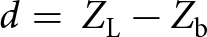
The annual terminus position time series show that 54 of the 55 lake-terminating glaciers retreated over 1984–2021 (Fig. 4). The only glacier to advance is Hole in The Wall Glacier near Juneau, AK (RGI60-01.27102), which advanced 263 m (5.8 m a−1). Hole in the Wall Glacier is a distributary branch of Taku Glacier, whose multi-decadal tidewater advance diverging from regional average behavior is well-documented (McNeil, Reference McNeil2020). The median retreat over this period was 2.1 km (mean = 2.4 km), with the interquartile range (IQR) spanning from 1.2 to 3.1 km. The median retreat rate over the 1984–2018 period was 60 m a−1 (mean = 81 m a−1) with the IQR spanning 35–89 m a−1 (Table S2). We note that the above retreat rates do not exactly correspond to the retreat distances because retreat rates are determined via a fit line while retreat distance is a simple difference between the first and last lengths. We use a 2018 end date here for consistency with lake area change data discussed in later analyses, as well as consistency with the input velocity datasets (Section 2.3). The fastest observed retreat rates (−751 m a−1 over 2009–18) are found at East Yakutat Glacier (RGI60-01.12645), which retreated ∼5.5 km since 2013 (750 m a−1) when the east and west glacier branches separated. Several glaciers demonstrate non-monotonic retreat due to period readvances due to surging (e.g. Bering Glacier; RGI60-01.13635; Fig. 4c orange line). Other glaciers (e.g. Grand Plateau—Alsek; RGI60-01.23655; Fig. 4d pink line) show stepped retreat, with large changes in terminus position between annual images, sometimes surrounded by periods of slower change.
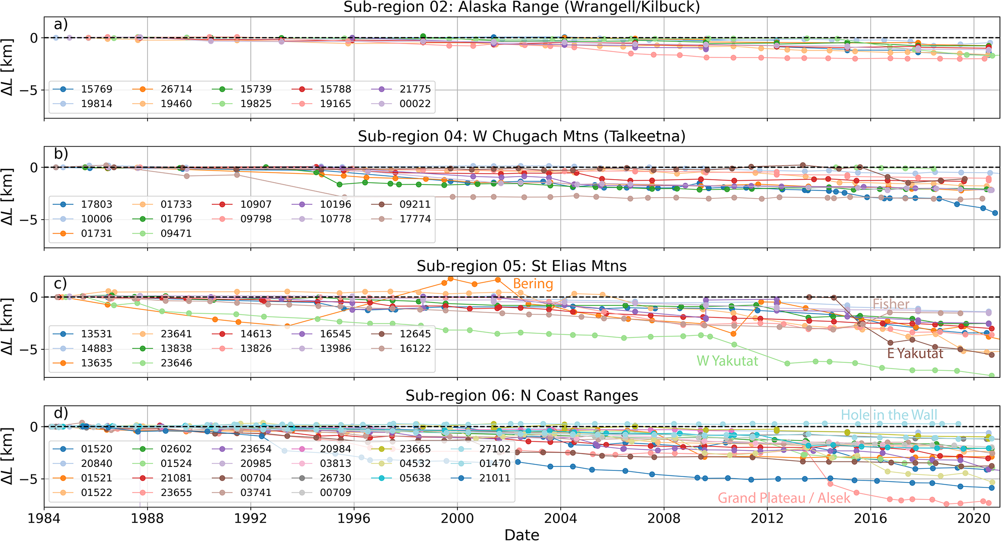
Figure 4. Length change (ΔL) time series for the 55 lake-terminating glaciers in this study, for (a) RGI subregion 01-02 (Alaska Range); (b) subregion 01-04 (W Chugach Mtns); (c) subregion 01-05 (St Elias Mtns); and (d) subregion 01-06 (N Coast Ranges). Negative length change indicates retreat. The legend in the lower left of each panel contains the RGI IDs for each glacier, where the leading ‘RGI60-01’. has been truncated.
The southeastern portion of the study area underwent more pronounced retreat, with RGI Region 01 subregions 05 and 06 (respectively St Elias Mountains and Northern Coast Ranges) retreating more on average than other locations (Fig. 4). In particular, higher retreat rates (>100 m a−1) are clustered in southeast Alaska’s Fairweather Range and Juneau Icefield, with the rest of the study area featuring a mix of glaciers retreating slowly (0–50 m a−1) or at intermediate rates (50–100 m a−1) with no obvious spatial coherence for either the 2009–18 period used for frontal ablation estimates (Fig. 5) or the full 1984–2021 study period (Fig. S6) retreat rates.
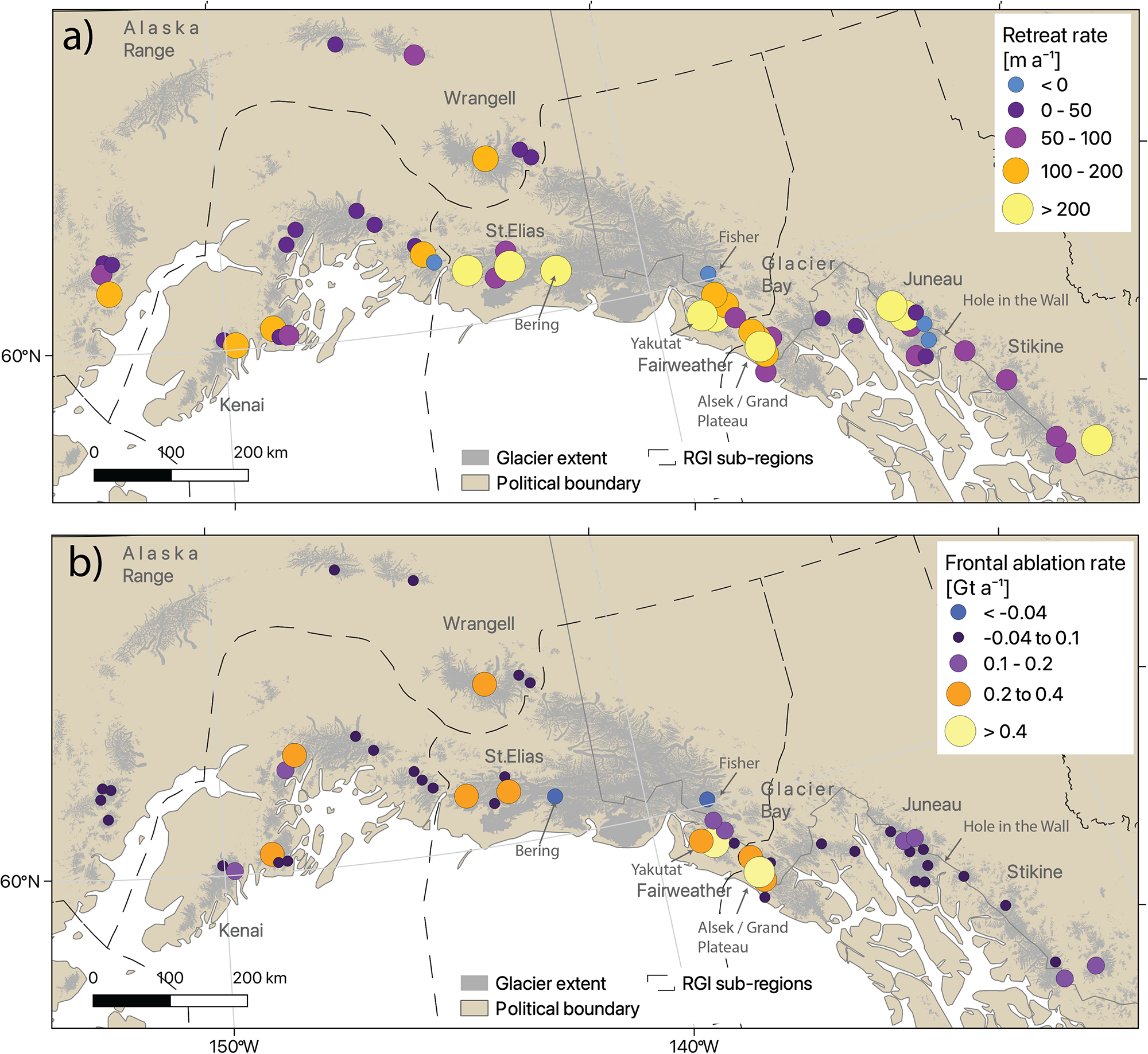
Figure 5. (a) Spatial distribution of retreat rates (2009–18) and (b) frontal ablation rates on lake-terminating glaciers across RGI region 01. A version of this figure using full-record retreat rates to calculate frontal ablation is shown in Figure S6. Map is projected in Alaska Albers (EPSG:3338).
3.2. Temporal variations in lake-terminating glacier retreat rates
The annual resolution of the glacier length time series allows investigation of changes in the rates of glacier retreat. On an individual glacier basis, we found widely varying behavior. Of the 49 study glaciers that were lake-terminating throughout the entire 1984–2021 study period (i.e. excluding 6 glaciers that either developed or detached from their proglacial lake over the study period), 12 (24%) increased their rate of retreat across the three decadal periods, while the rate of retreat progressively slowed (or even changed to advance) for 4 (8%) glaciers (Fig. S7). For the remaining glaciers, 17 (35%) accelerated their retreat rate before slowing, while 16 (33%) slowed then accelerated their retreat rate.
Analyzing all 55 study glaciers together, the median retreat rate increased by 123% (30−67 m a−1) from the 1986–98 period to the 2009–18 period (Fig. 6; Table S2). The retreat value of every percentile became more negative (Table S2), indicating that the retreat rates of both the slowly and rapidly changing glaciers are accelerating. However, both metrics of regional inter-period retreat rate variability (IQR and span [5–95%]) increased over time, indicating a widening divide between the fastest and slowest retreating glaciers.
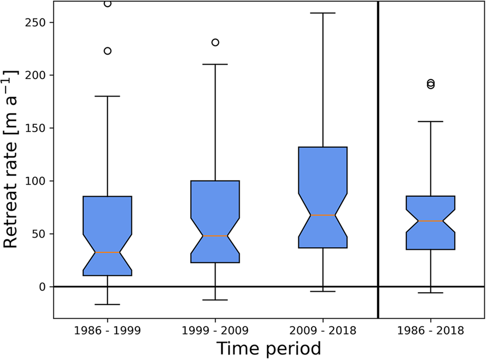
Figure 6. Box and whisker plots depicting retreat rates for the 55 study glaciers for the various periods, as well as the entire study period. The horizontal black line delineates retreat (rates > 0) from advance (rates < 0).
3.3. Estimates of frontal ablation
By combining our 2009–18 average retreat rates and existing geospatial datasets for ice thickness and velocity, we estimated a median frontal ablation rate of 0.04 Gt a−1 (IQR = 0.01–0.15) for the 55 lake-terminating study glaciers. Frontal ablation varies widely between different glaciers, with two glaciers losing ≥0.5 Gt a−1 to frontal ablation (East Yakutat Glacier, RGI60-01.12645; Grand Plateau—Alsek Glacier, RGI60-01.23655). Eight glaciers have frontal ablation rates between 0.2–0.5 Gt a−1 and nine have frontal ablation rates between 0.1–0.2 Gt a−1. The majority of study glaciers (58%; n = 32) have frontal ablation rates between −0.01 to 0.1 Gt a−1 (Figure S8). Negative values of F imply nonphysical mass gain through ice accretion at the terminus, which we do not expect in this setting. Instead, negative F values reflect improper closure of the mass budget below the flux gate, due to uncertainties in the input datasets (Section 2.4), the assumed terminal surface mass balance (Section 2.3; Fig. S4), and/or temporal mismatch between input datasets. We thus take the small negative estimates described above to reflect essentially zero mass loss through frontal ablation. Two glaciers (Bering Glacier and Fisher Glacier; RGI60-01.16122) have substantially negative F estimates of −0.56 and −0.15 Gt a−1. Both of these glaciers underwent surges in the early part of the 2009–18 retreat rate period used for frontal ablation but had reached quiescence by the 2017–18 date (Burgess and others, Reference Burgess, Forster, Larsen and Braun2012; Partington, Reference Partington2023) described by the Millan and others (Reference Millan, Mouginot, Rabatel and Morlighem2022) surface velocities, resulting in low ice discharge (Q in) estimates. For Fisher Glacier, Eqn (2) produces a negative frontal ablation (signifying ice accretion) to explain the glacier’s advance, which is actually due to surge dynamics and should thus be ignored as a nonphysical result. The piedmont geometry of Bering Glacier results in a very large surface areas below its flux gate, and our assumed high melt rate of  $\dot b$ = −10 m a−1 results in a significant overestimate of surface melt, which produces a negative frontal ablation estimate because the calculated surface melt is greater than the incoming ice discharge. This error is exacerbated by the Q in estimate being biased low due to the above-referenced timing mismatch between its recent surge and the velocity dataset. For Bering Glacier, we estimate 1.96 Gt a−1 loss to surface melt below the flux gate (Q melt), and either reducing the Q melt by 40% (corresponding to $\dot b$ = − 7.1 m a−1) or increasing Q in seventeen-fold is required to produce the physically expected F > 0 Gt a−1 for this glacier. In all likelihood, both terms are likely in error, as the glacier’s terminal $\dot b$ was estimated to be close to −8 m a−1 over 1951–2011 (Tangborn, Reference Tangborn2013) and a recent study showed the Millan and others (Reference Millan, Mouginot, Rabatel and Morlighem2022) ice thickness estimates (an input to Q in) had high uncertainty for Sít’ Tlein (Malaspina Glacier), a nearby glacier with similar piedmont morphology (Tober, Reference Tober2023). Bering Glacier is an especially challenging case for the application of Eqn (2) due to its surge history and large, unconstrained piedmont lobe, and we thus argue that a nonphysical F estimate at this one glacier does not invalidates the rest of the data we present here.
Summed across all study glaciers with positive F values, the collective rate of mass loss through frontal ablation is 6.1 Gt a−1 over 2009–18. Using the slower 1984–2021 retreat rates results in a regional frontal ablation loss of 4.9 Gt a−1, which sums to 183 Gt if the rate is held constant for the study period. Our study glaciers represent 83% of the region’s lake-terminating glaciers as identified by the RGI v6 by area, but they are the largest or fastest retreating glaciers. We therefore suspect that the remaining 27% of RGI region 01 lake-terminating glacier area will increase regional frontal ablation loss by substantially less than 27%.
Varying frontal ablation rates are found throughout the region, with little evidence for large-scale spatial patterns (Fig. 5b). However, the Fairweather Range features a high density of glaciers with large frontal ablation rates (e.g. Yakutat, Grand Plateau and Alsek glaciers). Additionally, the interior ranges (i.e. Alaska & Wrangell) do not host many glaciers with high frontal ablation rates (Fig. 5b).
3.4. Comparing lake- and marine-terminating glaciers
Comparing lake- and marine-terminating glaciers, we find differing patterns of retreat and overlapping frontal ablation distributions. McNabb and others (Reference McNabb, Hock and Huss2015) found that only ∼60% (16 of 27) of marine-terminating glaciers retreated over 1984–2013, while we show that nearly all (98%, 54 of 55) lake-terminating glaciers retreated over the same timespan (Fig. 7). On average, marine-terminating glaciers retreated ∼20% slower than lake-terminating glaciers in this region, with a mean marine-terminating retreat rate of 47 m a−1 in comparison to the 58 m a−1 mean rate for lake-terminating glaciers. Comparing median rates, an even starker picture emerges, with marine-terminating glaciers retreating only 2 m a−1 on average, while the median lake-terminating glacier retreat rate was 51 m a−1. The large discrepancy between mean and median retreat rates for marine-terminating glaciers is driven by the collapse of Columbia Glacier (RGI60-01.10689), which retreated 500 m a−1 on average over the study period.
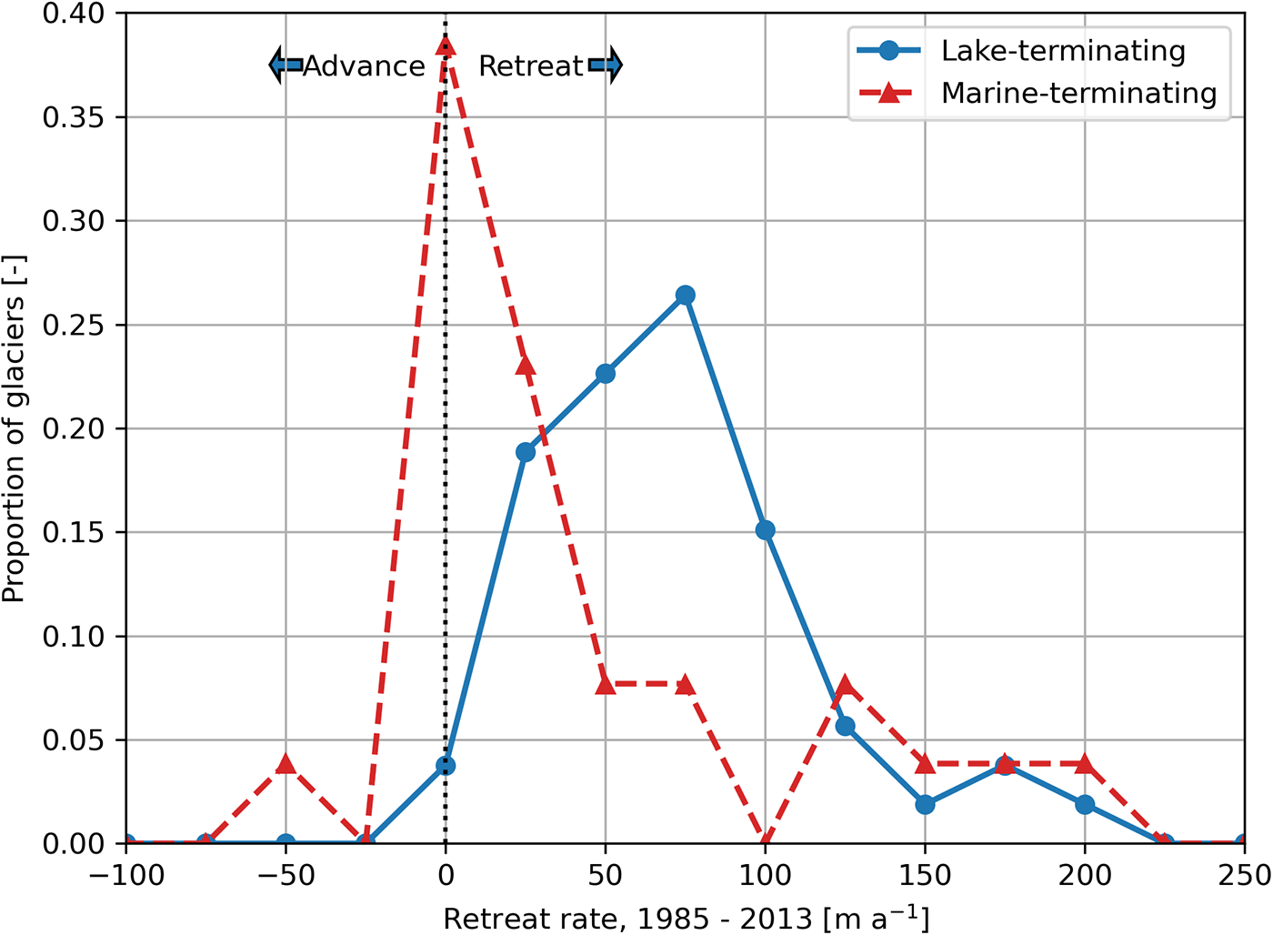
Figure 7. Histograms depicting the average retreat rate of lake-terminating (blue) and marine-terminating (red) glacier retreat from 1984 to 2013 (aligned with the McNabb and others (Reference McNabb, Hock and Huss2015) marine-terminating dataset). Positive values indicate retreat while negative values represent advance. The marine-terminating Columbia Glacier retreat rate of 500 m a-1 is not shown for clarity.
Marine-terminating glaciers generally have higher rates of frontal ablation than lake-terminating glaciers, with the median frontal ablation rate for marine-terminating glaciers (0.27 Gt a−1) an order of magnitude larger than the median lake-terminating rate (0.04 Gt a−1). However, substantial overlap exists between the tails of each frontal ablation distribution, with the 75th percentile lake-terminating frontal ablation rate (0.15 Gt a−1) exceeding the 25th percentile marine-terminating frontal ablation rate (0.10 Gt a−1; Figure S8). Physically, this means that while frontal ablation rates are on average higher for marine-terminating glaciers, the lake-terminating glaciers with the highest frontal ablation rates (top quarter) lose more mass through the terminus than the marine-terminating glaciers with the lowest frontal ablation rates (bottom quarter). Comparing the slopes of the outlier-resistant Theil–Sen best fit lines, we find that a marine-terminating glacier on average loses 4.9 times more mass through frontal ablation than a lake-terminating glacier of equivalent area (Fig. 8a; marine-terminating slope = 10−3 Gt a−1 km−2; lake-terminating slope = 2 × 10⁻⁴ Gt a−1 km−2). However, lake-terminating glaciers retreat faster for a given frontal ablation rate (Fig. 8b).
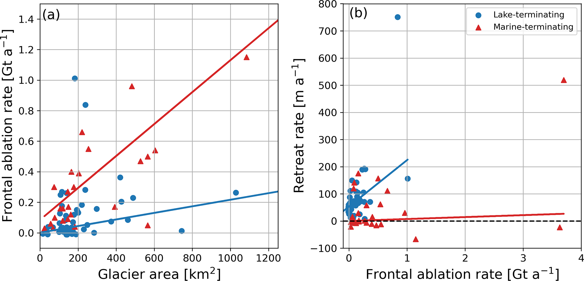
Figure 8. (a) Glacier area versus frontal ablation rate for lake-terminating (blue circles) and marine-terminating (red triangles) glaciers. (b) Study period average frontal ablation versus retreat rate for lake-terminating (blue) and marine-terminating (red) glaciers. Marine-terminating data is from McNabb and others (Reference McNabb, Hock and Huss2015). Marine-terminating glaciers with outlying frontal ablation rates and/or areas (Columbia Glacier, F = 3.7 Gt a-1, area = 944 km2; Hubbard Glacier, F = 3.6 Gt a-1, area = 3402 km2) as well as lake-terminating glaciers with substantially negative F values (discussed in text; Bering Glacier, F = −0.56 Gt a-1, area = 3025 km2; Fisher Glaciers, F = −0.15 Gt a-1, area = 441 km) are not shown for clarity.
3.5. Investigating potential physical drivers of lake-terminating retreat and frontal ablation
We find several associations between environmental variables and both retreat and frontal ablation rates. Across Alaska, proglacial lake area has increased by 85% (543−1006 km2) since 1984 (Rick and others, Reference Rick, McGrath, Armstrong and McCoy2022). In situ data show that water depth generally increases with lake area (Cook and Quincey, Reference Cook and Quincey2015), and we find that the predicted water depth (d) in the terminal 2 km for each glacier scales with the 2018 lake area (τ = 0.32, p < 0.01). Retreat and frontal ablation rates over 2009–18 are positively associated with lake area (respectively τ = 0.23, p < 0.01; τ = 0.51, p < 0.01; Fig. 9a) and near-terminus water depth (respectively τ = 0.22, p = 0.02; τ = 0.40, p < 0.01; Fig. 9b). Physically, the latter association means that glaciers with deeper water near the terminus on average experience higher rates of frontal ablation than others. There also appears to be an association between the length of the terminal overeepening and frontal ablation rates (Fig. 9c), suggesting that the glaciers that are presently losing the most mass to frontal ablation also have the most to lose over the long term.
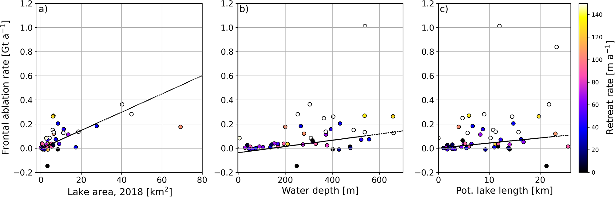
Figure 9. (a) Estimates of 2018 lake area versus frontal ablation rate for Alaska’s lake-terminating glaciers over 2009–18. Color bar indicates rate of glacier retreat, with warmer colors (e.g. yellow and white) indicating faster rates over 2009–18. (b) Median potential lake depth versus rates of frontal ablation. (c) Length to the point where the glacier bed rises above the proglacial lake elevation, using the best guess ice thickness.
3.6. Projecting transition from lake- to land-terminating glaciers
When lake-terminating glaciers recede from their terminal overdeepenings, they transition to land-terminating and therefore lose frontal ablation as a mass loss term. To provide a first-order estimate for when these glaciers transition to a land-terminating state, we estimate the median distance from a lake-terminating glacier’s terminus to the first point where the glacier bed rises above the lake surface elevation (at the time of the GLO-90 DEM, corresponding to 2011–15). We find a median distance of 9.0 km to the end of the terminal overdeepening, though on a glacier-by-glacier basis, substantial variation exists in both terminal overdeepening lengths (IQR = 4.6–14 km; Fig. 10a) and retreat rates (IQR = 37–144 m a−1), which yields a wide range in the projected time to transition to a land-terminating condition (t land; IQR = 38–177 years; median = 74 years) based on 2009–18 retreat rates (Fig. 10b). For some glaciers, it could be centuries before the glacier is land-terminating if they continue to retreat at their 2009–18 rate, with the 90th percentile t land being 279 years. The potential distance at which a glacier’s bed rises above the lake surface elevation varies by 4.9 km (51%) on average due to uncertainty in ice thickness, with a larger range found for glaciers with larger glaciers with lower surface slopes. Using the low- and high-end estimates of ice thickness result in median t land values ranging from 48 to 91 years using the 2009–18 retreat rates. Using the slower retreat rates averaged over the full 1984–2021 study period gives a median t land value of 118 years using the middle ice thickness estimate.
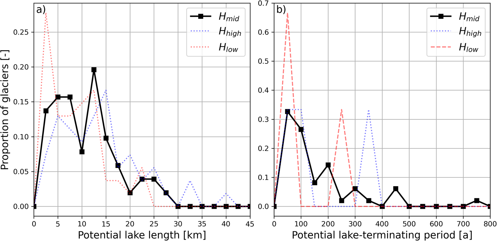
Figure 10. (a) Distribution of distance upstream from the terminus along centerline profiles to the point where the glacier bed elevation is above the current lake elevation using the Millan and others (Reference Millan, Mouginot, Rabatel and Morlighem2022) ice thickness distribution (black solid line) as well as upper- (blue dashed) and lower-end (red dashed) estimates based on the pixel-wise thickness uncertainty provided by that dataset. (b) Distribution of the time required for a glacier to reach these points if glacier retreat continues at the 2009–18 rate. As in (a), line style reflects whether the middle, upper-, and lower-end ice thickness estimate from Millan and others (Reference Millan, Mouginot, Rabatel and Morlighem2022) is used in the calculation.
4. Discussion
Above, we estimated retreat and frontal ablation rates for Alaska and northwest Canada’s lake-terminating glaciers, compared these values to the regions marine-terminating glaciers, investigated associations between these rates and lake characteristics, and estimated how long the glaciers will remain lake-terminating using existing geospatial datasets. Below, we interpret these results and put them in their scientific context. First, we delve deeper into the factors behind the region’s widely varying lake-terminating frontal ablation rates and identify glaciers diverging from the regional norm. Later, we attempt to reconcile the region’s disparate lake- and marine-terminating glaciers thinning rates given our results and the area’s glacier history. Finally, we look forward using the example of Patagonia and our estimates for the duration over which our study glaciers will remain in contact with their proglacial lakes to envisage the future of Alaska’s lake-terminating glaciers.
4.1. Parsing contributions to frontal ablation
To develop a greater understanding of what sets the rate of frontal ablation across our lake-terminating study glaciers, we dissect Eqns (1) and (2) to investigate the absolute and relative contributions to F of ice flux through the flux gate ( ${Q_{\text{in}}}$), terminus retreat $A\frac{{dL}}{{dt}}$ ( ${Q_{\text{ret}}}$) and surface melt in the region between the flux gate and terminus ( ${Q_{\text{melt}}} = \dot bS$). This analysis allows discrimination of cases in which a high frontal ablation rate is produced from the disintegration of a slow-moving tongue ( ${Q_{\text{ret}}} \gg {Q_{\text{in}}}$) from cases of glaciers that are closer to steady state ( ${Q_{\text{ret}}} \approx 0$) despite high mass loss through frontal ablation ( ${Q_{\text{in}}} \gg {Q_{\text{ret}}}$). We interpret a high ratio of ${Q_{\text{in}}}/{Q_{\text{ret}}}$ (i.e. ≫1) to reflect ‘active’ frontal ablation where the high ice discharge may allow the upstream glacier to respond more sensitively to terminus conditions via positive feedbacks between frontal ablation and glacier geometry. By contrast, a large F can also be obtained by a high ${Q_{\text{ret}}}{\text{ }}$and low Q in ( $\frac{{{Q_{\text{in}}}}}{{A\frac{{dL}}{{dt}}}} \ll 1$), which we consider ‘passive’ frontal ablation because it is driven more by a lack of Q in across the flux gate (the integral of upstream surface mass balance) rather than anything occurring at the glacier terminus. In most cases, we find terminus retreat and incoming ice discharge contribute approximately equally to our F estimates (Fig. 11a 1:1 line), suggesting active processes at the glacier terminus and as well as glacier-wide processes share responsibility for frontal ablation on the majority of study glaciers. However, several outliers from this relationship exist, suggesting that these glaciers are undergoing substantially different frontal ablation processes than the regional norm. Prominent examples where terminus retreat dominates F are Bering Glacier (RGI60-01.13635) and East Yakutat Glacier (RGI60-01.12645). As discussed in Section 3.3, Bering Glacier underwent a surge during 2008–11 (Burgess and others, Reference Burgess, Forster, Larsen and Braun2012), resulting in an ‘overextended’ terminus that subsequently retreated and slow surface velocities during the 2009–18 period for F estimations. East Yakutat Glacier had a floating tongue that began to disintegrate in 2010 (Trüssel and others, Reference Trüssel, Truffer, Hock, Motyka, Huss and Zhang2015). The glacier drains the low-elevation Yakutat Icefield, whose highest reaches are at times below the end-of-summer snowline, leaving the glacier with little to no accumulation zone (Trüssel and others, Reference Trüssel, Truffer, Hock, Motyka, Huss and Zhang2015). In both of these cases, the glaciers have insufficient accumulation area to provide the high mass flux required to balance melt in their extensive low lying regions, and would thus undergo substantial retreat even in the absence of calving and subaqueous melt. Indeed, Trüssel and others (Reference Trüssel, Truffer, Hock, Motyka, Huss and Zhang2015) found that incorporating a frontal ablation parameterization had little effect on the evolution of Yakutat Glacier, with its 21st-century evolution driven largely by surface mass balance.
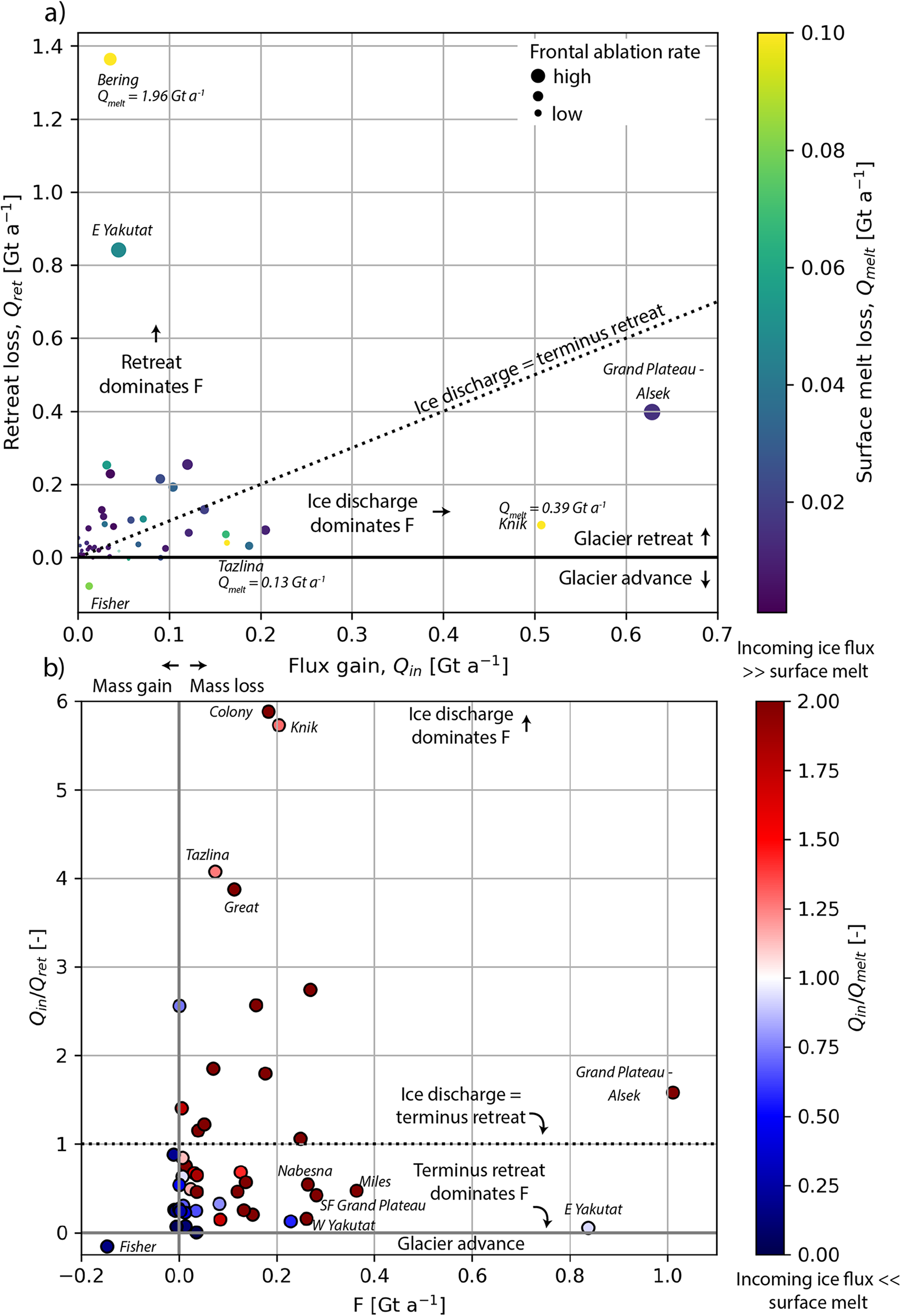
Figure 11. Parsing the contribution of frontal ablation in terms of the (a) absolute and (b) relative values of terms in Eqn (2). In (a), points are scaled by the estimated frontal ablation rate (F) and colored by the mass loss to surface melt in the region below the flux gate (Q melt). In (b), the y-coordinate of each point reflects the balance of ice discharge Q in and terminus retreat (Q ret) at setting the frontal ablation rate. A value of 1 on this axis indicates Q in and  ${Q_{\text{ret}}}$ contribute equally to F, where values >>1 and 0 respectively indicate dominance of Q in or Q ret in setting F. The color axis in (b) shows the proportion of Q in is expected to be lost to surface melt between the flux gate and terminus. The signs of Q ret and Q melt are inverted for clarity on this plot, but they are in fact negative in almost all cases, as shown in Eqn (1). On both panels, the names of outlying glaciers are given in gray text. In (b), Bering Glacier is omitted due to its substantially negative F estimate, discussed in Section 3.3.
In most cases surface melt below the flux gate is substantially smaller than the incoming ice flux (blue points on Fig. 11a, red dots on Fig. 11b), even with the conservatively assumed terminal surface mass balance rate  $\dot b$ = −10 m a−1. However, there are cases where ${Q_{\text{melt}}} /gt {Q_{\text{in}}}$ (blue points on Fig. 11b). These cases could result from our assumed melt rate being too high or modeled ice thickness too low, which will produce unrealistically low frontal ablation rates. However, these cases could also be explained by glacier retreat on these glaciers being dominated by declining surface mass balance over the whole glacier, such that the incoming ice discharge ( ${Q_{\text{in}}}$; which integrates the upstream surface mass balance) in insufficient to balance melt in the terminal region. If the second explanation were true, these glaciers would essentially act like land-terminating glaciers, with frontal ablation playing a limited role in their ongoing retreat.
4.2. Contextualizing differences between lake- and marine-terminating glaciers
In other studies, lake-terminating glaciers are associated with higher rates of mass loss than land-terminating glaciers (King and others, Reference King, Bhattacharya, Bhambri and Bolch2019; Maurer and others, Reference Maurer, Schaefer, Rupper and Corley2019) as well as marine-terminating glaciers (Larsen and others, Reference Larsen2015). During the 2000–15 time-period, King and others (Reference King, Bhattacharya, Bhambri and Bolch2019) found that lake-terminating glaciers in the Himalaya experienced nearly 1.5 times more negative mass balance than land-terminating glaciers, and that this discrepancy had increased over time. While substantial differences exist between Himalayan and Alaskan glaciers, and covariance between terminus type and other attributes may exist (e.g. elevation, ice thickness) this study suggests mass loss enhancement in glaciers terminating in lakes. The Larsen and others (Reference Larsen2015) study used airborne altimetry to show that lake-terminating glaciers contribute four times as much to total Alaskan glacier mass loss than marine-terminating glaciers (6% vs 24%). Many of these studies suggest frontal ablation as a causative mechanism to explain differences in mass loss rates between terminus classes, but systematic analyses of the mass lost through frontal ablation in lake-terminating systems remain sparse (Minowa and others, Reference Minowa, Schaefer, Sugiyama, Sakakibara and Skvarca2021). Our dataset allows a direct estimate of the equivalent thinning frontal ablation on study glaciers would produce if the mass loss were spread uniformly across a glacier’s entire surface area. The median equivalent thinning due to frontal ablation values is 0.25 m w.e. a−1 (IQR = 0.06–0.70 m w.e. a−1) for our study glaciers. Converting the 2010–20 total mass loss data from Hugonnet and others (Reference Hugonnet2021; which includes the effects of both surface melt and frontal ablation) to average thinning rates (dividing volume loss by surface area), we find a median overall thinning rate for our lake-terminating study glaciers of 1.21 m w.e. a−1 (iIQR = 0.94–1.55 m w.e. a−1). We do not compute percentages of total loss due to frontal ablation because our frontal ablation estimates do not necessarily reflect a mass imbalance—a glacier in steady state could still have high mass loss through the terminus. However, comparing the relative magnitude of the mass loss terms, we show that mass loss from frontal ablation could be an important process in shaping the future evolution of the region’s lake-terminating glaciers.
Considering the regional sum of positive F vales (6.1 Gt a−1), we compute an area-weighted equivalent thinning rate of 0.62 m w.e. a−1 by dividing the F sum by the surface area of glaciers with positive F values (9700 km2; notably, notably excluding Bering Glacier, the largest glacier in the dataset). This value is 45% of Alaska’s area-weighted equivalent thinning rate for marine-terminating glaciers (1.37 m w.e. a−1; McNabb and others, Reference McNabb, Hock and Huss2015).
Comparing median retreat rates, Alaska’s lake-terminating glaciers retreated substantially faster than their marine-terminating counterparts (Fig. 7; 51 m a−1 vs 2 m a−1) over 1984–2013 despite lake-terminating glaciers losing about five times less mass through frontal ablation than a marine-terminating glacier of the same surface area. By investigating total mass loss over 2010–2020 (Hugonnet, Reference Hugonnet2021), we find that, while lake-terminating glaciers lose less mass to frontal ablation than marine-terminating glaciers, they are losing more mass overall. Lake-terminating study glaciers have a median total mass loss of 0.19 Gt a−1 (IQR = 0.11–0.36 Gt a−1) compared with 0.08 Gt a−1 (0.03–0.29 Gt a−1) for marine-terminating study glaciers.
Systematic differences between the lake- and marine-terminating glacier-wide mass balance due to differences in the hypsometry and AAR could partly explain the apparent variation in retreat sensitivity to frontal ablation rates. Many of Alaska’s marine-terminating glaciers underwent catastrophic tidewater retreat in the 19th and 20th centuries, prior to our study period, resulting in relatively stable states with high AARs in the late 20th century (Larsen and others, Reference Larsen2015). Many of the current lake-terminating glaciers were land-terminating (or terminating in small and likely shallow lakes) during the same time period and may thus have responded more slowly to climate change because they lacked the additional mass loss term of frontal ablation, resulting in the glaciers being ‘overextended’ relative to the modern climate with low AARs. Indeed, the median AAR for our lake-terminating study glaciers is 0.46 (IQR = 0.34–0.52) compared with 0.59 (0.49–0.73) for marine-terminating study glaciers, and this effect persists when dividing glaciers into their RGI subregions to account for potential climatic differences between lake- and marine-terminating glaciers (Fig. 12). These findings are similar to those of Patagonia, where lake-terminating glaciers were found to have systematically lower AARs (0.63 vs 0.85) and flatter ablation zones than their marine-terminating counterparts (Minowa and others, Reference Minowa, Schaefer, Sugiyama, Sakakibara and Skvarca2021). Thus, our comparison of lake- and marine-terminating glaciers may in some ways not reflect a difference in process, but a difference in their phase in the ‘tidewater glacier cycle’ (Post and others, Reference Post, O’Neel, Motyka and Streveler2011) and resultant larger relative ablation areas that make lake-terminating glaciers respond more sensitively to modern climate warming. Indeed, in subregion 06 (Northern Coast Ranges) where AAR distributions are similar between lake- and marine-terminating glaciers (Fig. 12), median retreat rates between terminus classes are much more closer than for the entire Alaska region (46 m a−1 retreat for marine-terminating glaciers vs 66 m a−1 for lake-terminating glaciers over 1985–2013, respectively, compared with 2 and 51 m a−1 for the entire region).

Figure 12. Summary of accumulation area ratio differences between lake- (blue) and marine-terminating (red) study glaciers. Glaciers are divided into RGI subregions (Figure 1) to control for climate regime. Subregions are defined as follows: 02 = Alaska Range, 04 = Western Chugach, 05 = St Elias; 06 = Northern Coast Ranges.
Nevertheless, our findings show that frontal ablation rates on lake-terminating glaciers can be comparable to those seen on marine-terminating glaciers. Frontal ablation may therefore be an important mass loss term for lake-terminating glaciers despite the presence of relatively cold water and the absence of a turbulent buoyant plume melt in the lakes (Benn and others, Reference Benn, Warren and Mottram2007a; Truffer and Motyka, Reference Truffer and Motyka2016). The proliferation of proglacial lakes across Alaska coincides with accelerated thinning of Alaska glaciers (0.65 m a−1 over 2000–04 to 1.24 m a−1 over 2015–19; Hugonnet, Reference Hugonnet2021) and retreat rates of lake-terminating glaciers. This correspondence has led some authors (e.g. King and others, Reference King, Bhattacharya, Bhambri and Bolch2019) to postulate that the lakes themselves are causing the enhanced mass loss, but systematic differences in quantities such as ice thickness, AAR and elevation between terminus classes (e.g. Yang, Reference Yang2022) can confound such analyses. Estimates of mass loss through frontal ablation in freshwater systems over large spatial scales have only recently becoming available, with ∼7 Gt a−1 lost through lacustrine termini in Patagonia (Minowa and others, Reference Minowa, Schaefer, Sugiyama, Sakakibara and Skvarca2021). In the Himalayas, recent work found that traditional geodetic estimates underpredicted mass loss by ∼ 7% because they did not account for subaqueous mass loss (Zhang, Reference Zhang2023), but this study is based upon uncertain lake area-volume scaling. Together with these previous studies, our estimates of lake-terminating frontal ablation rates suggest that frontal ablation in Alaska currently is an important mass loss process for some lake-terminating glaciers.
4.3. Future evolution of Alaska’s lake-terminating glaciers: analog in Patagonia?
Alaska’s ice-marginal lakes grew rapidly over the past 40 years (increasing in area by 85% between 1984 and 2019 to now cover 1000 km2), and there is no sign of this trend slowing (Rick and others, Reference Rick, McGrath, Armstrong and McCoy2022). Using the modern lake surface elevation, ice thickness estimates and observed rates of glacier retreat, our data suggest that Alaska’s lake-terminating glaciers will not retreat from their terminal overdeepenings and become land-terminating for many decades (median = 74 a; IQR = 38–177 a) if the glaciers continue to retreat at their 2009–18 retreat rates.
Given our findings, the growth of proglacial lakes may have important consequences for the evolution of the region’s lake-terminating glaciers. Larger lakes tend to be deeper (Cook and Quincey, Reference Cook and Quincey2015; Zhang, Reference Zhang2023). We find that frontal ablation rates tend to increase with proglacial lake area and water depth (Figs. 9a-b), suggesting that lake-terminating glacier mass loss through frontal ablation will only increase as proglacial lakes grow and deepen. Glaciers could transition to a land-terminating condition earlier than projected above if future retreat rates are faster than those observed over the past decades.
While factors such as wind-driven overturn circulation strength and changes in water fluxes are likely important, it is plausible to imagine that as proglacial lake area increases, more surface area is available to absorb solar radiation, potentially warming surface waters and enhancing rates of subaqueous melt (Trüssel and others, Reference Trüssel, Truffer, Hock, Motyka, Huss and Zhang2015). Sparse in situ observations in Alaska proglacial lakes show surface water temperatures <3°C (Boyce and others, Reference Boyce, Motyka and Truffer2007), yet observations on the larger proglacial lakes of Patagonia show water surface temperatures as high as 8°C (Sugiyama, Reference Sugiyama2016). Further, ASTER remote-sensing data in other parts of the world suggest that proglacial lakes could be warmer than the often-assumed uniform low (∼1°C) temperature (Dye and others, Reference Dye, Bryant, Dodd, Falcini and Rippin2021). Thus, if Alaska’s proglacial lakes warm towards Patagonian levels as they continue to grow, increased frontal ablation rates through enhanced subaqueous melt are possible.
In Patagonia, the average (meaning median) lake-terminating glacier lost 0.08 Gt a−1 (IQR = 0.02–0.25 Gt a−1) through frontal ablation over 2000–19 (Minowa and others, Reference Minowa, Schaefer, Sugiyama, Sakakibara and Skvarca2021) roughly double the rates we document in Alaska (median = 0.04 Gt a−1; IQR = 0.01–0.15 Gt a−1) over 2009–18. In Patagonia, there is some evidence that frontal ablation rates increase superlinearly with increasing glacier area (best-fitting power-law area exponent = 1.2; Fig. 13 thick orange line) while Alaska’s lake-terminating frontal ablation rates increase sublinearly (area exponent = 0.46). If instead a linear fit is applied to the data, we find the slope of the best-fit line to Patagonia data is three times steeper than that for Alaska (Fig. 13 thin lines). The explained variance (R 2) is substantially higher for the power-law fits in both cases (0.60 vs 0.42 for Patagonia; 0.07 vs −0.10 for Alaska), suggesting nonlinear relationships between glacier area and frontal ablation in both regions. Regardless of the functional form of the fit line, we find substantial overlap between Alaska and Patagonia frontal ablation rates for glaciers <500 km2, with the most pronounced difference seen for the regions’ largest glaciers (Fig. 13). The termini of many Patagonia glaciers are steep and fast flowing due to regional topography (Minowa and others, Reference Minowa, Schaefer and Skvarca2023), which could partly explain the differences in frontal ablation rates. However, the Patagonia glaciers with the highest frontal ablation rates terminate in lakes orders of magnitude larger than the Alaska glaciers (Fig. 13), which could have a substantial effect as well. As Alaska’s lake-terminating glaciers continue to retreat, they move into more confined valleys, which could promote steepening and faster terminus velocities. This dynamic, in addition to their growing (and perhaps warming) proglacial lakes, could mean that Alaska’s future lake-terminating glaciers look much more similar to the Patagonian example than they do at present.
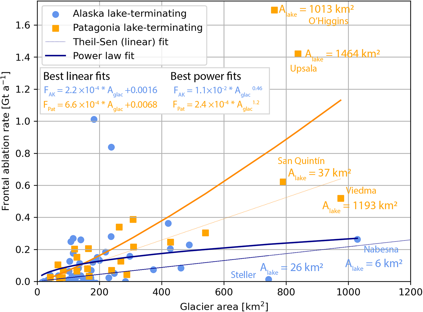
Figure 13. Comparison of frontal ablation rates between Alaska (blue circles) and Patagonia (orange squares) lake-terminating glaciers as a function of glacier area. Equations for the Sen slope linear best fit to data from each region are displayed in the upper left, where the units of frontal ablation and glacier area (Aglac) are respectively Gt a-1 and km2. Lake area for large glaciers are indicated in colored text. Data from Patagonia are reported in Minowa and others (Reference Minowa, Schaefer, Sugiyama, Sakakibara and Skvarca2021).
5. Conclusions
The role of proglacial lakes in glacier change is receiving more attention as proglacial lakes proliferate and grow around the world, yet estimates of additional mass loss due to these lakes are sparse. We investigate Alaska and northwestern Canada, a region with rapid proglacial lake expansion, and find that lake-terminating glaciers retreated a median rate of 60 m a−1 (IQR = 35–89 m a−1) over 1984–2018 and lost 0.04 Gt a−1 (IQR = 0.01–0.15 Gt a−1) of ice through frontal ablation over 2009–18. While the data we report here do not necessarily reflect an imbalance, mass loss through frontal ablation is significant when compared the 2010–20 median total mass loss rate of 0.19 Gt a−1 for our study glaciers. The region’s lake-terminating glaciers retreated substantially faster than its marine-terminating glaciers, despite lake-terminating glaciers losing five times less mass through frontal ablation than marine-terminating glaciers of equivalent area (Fig. 8). The difference in retreat rates may be due to lake-terminating glaciers showing systematically lower AARs than the region’s marine-terminating glaciers (0.46 vs 0.59), which indicates they are more out of balance with the current climate. We compare our results with existing geospatial datasets and find positive relationships between frontal ablation and lake area and terminal water depth. Large lakes are associated with greater water depth, frontal ablation and retreat rates. As the region’s proglacial lakes continue to expand, they may warm and/or deepen, only increasing rates of mass loss though frontal ablation to become more similar to Patagonian glaciers. We find that most of the region’s lake-terminating glaciers will likely remain so for at least the remainder of this century, making enhanced understanding of frontal ablation critical for projecting the long-term evolution of Alaska’s lake-terminating glaciers. Our work provides a first-order estimate of losses to freshwater frontal ablation from remotely sensed datasets and shows that this has been an important mass loss process for many lake-terminating glaciers in the past and could continue to play an important role in the evolution of the region’s lake-terminating glaciers throughout the 21st century. The substantial mass lost through frontal ablation motivates its incorporation into models of glacier changes. Parameterizations of freshwater frontal ablation must differ from those applied in marine-terminating environments and should be based on detailed in situ observations such as proglacial lake bathymetry and hydrographic structure as well as subglacial topography. Constraining how lake-terminating frontal ablation processes operate at present and how they are likely to change in a warming climate could alter projections of glacier evolution with implications for management of future sea level rise, downstream water resources and aquatic ecosystems.
Supplementary material
The supplementary material for this article can be found at https://doi.org/10.1017/jog.2025.37
Data availability statement
Terminus positions and tabular results for each study glacier are aviable via Zenodo at https://doi.org/10.5281/zenodo.15241674
Ice thickness and velocity data are available from Millan and others (Reference Millan, Mouginot, Rabatel and Morlighem2022; https://doi.org/10.6096/1007). Overall glacier mass change is from Hugonnet and others (2021; https://doi.org/10.6096/13). Proglacial lake area data are from Rick and others (2022; https://doi.org/10.18739/A2MK6591G). Surface elevation data are from the Copernicus GLO90 digital elevation model (https://doi.org/10.5270/ESA-c5d3d65). Accumulation area ratios are provided by Zeller and others (accepted; https://dx.doi.org/10.5066/P1QHST6F). The Randolph Glacier Inventory is available at https://doi.org/10.5067/f6jmovy5navz.
Acknowledgements
This work was enabled by the data sharing and software development of many cryosphere community members (McNabb and others, Reference McNabb, Hock and Huss2015; RGI Consortium, 2017; Lea, Reference Lea2018; Gardner and others, Reference Gardner, Fahnestock and Scambos2022; Millan and others, Reference Millan, Mouginot, Rabatel and Morlighem2022). We gratefully acknowledge support from NSF-OPP-1821002, NSF-OPP-2334775, the Appalachian State University Honors College, and the Office of Student Research. Regine Hock aided in the interpretation of negative frontal ablation rates and provided suggestions on data presentation to improve the utility of our dataset for the global glacier modeling community. The detailed and constructive reviews provided by Scientific Editor Marius Schaefer, Will Kochtitzky, and one anonymous reviewer substantially improved the quality of this manuscript.
Author contributions
NC completed primary data generation, post processing, data analysis, drafting original manuscript text and text revision. WA secured funding, conceived project idea, performed geospatial data extraction, advised research direction, contributed to & edited the manuscript, and performed the bulk of the peer-reiew revisions. RM developed the dataset of frontal ablation for marine-terminating glaciers, provided discussion & feedback, and contributed to & edited the manuscript. EE provided discussion & feedback, and contributed to & edited the manuscript. DM supervised the development of the proglacial lake extent dataset, provided discussion & feedback, and contributed to & edited the manuscript. BR developed the dataset of proglacial lake extents, and provided discussion & feedback. JH developed a preliminary version of retreat time-series for lake-terminating glaciers. LBP provided discussion & feedback and edited the original manuscript.
Competing interests
The authors declare no competing interests.


 Open access