

Introduction
Measurement of the snow water equivalent (SWE) of a snowpack over a large spatial extent is crucial for forecasting snowmelt timing (Reference Luce, Tarboton and CooleyLuce and others, 1998) and calculating snowmelt volume (Reference Elder, Dozier and MichaelsenElder and others, 1991), among other applications. Direct measurement of SWE in mountain environments with remote sensing is theoretically possible, relying upon the sensitivity of radar backscatter to the water content and structure of the snowpack (Reference Shi and DozierShi and Dozier, 2000), but has proved extremely challenging in practice. Snow depth, in contrast, is the primary driver of spatial SWE variability, and is relatively straightforward to measure over large areas with remote-sensing techniques, in particular through differencing of surface elevations measured using airborne or ground-based lidar systems (Reference Deems, Painter and FinneganDeems and others, 2013). SWE is a function of bulk snow density and snow depth; thus, when used in combination with a regional snow density model (e.g. Reference Jonas, Marty and MagnussonJonas and others, 2009), lidar-altimetry-derived snow depths enable the calculation of SWE. Many commercially available lidar scanners operate at wavelengths that minimize the penetration of the laser light into the snowpack, making them ideally suited for measuring the surface of snow (Reference Dozier and PainterDozier and Painter, 2004).
As application of airborne and terrestrial laser scanning (ALS and TLS) techniques to the measurement of snow depth continues to grow (e.g. Reference Deems, Painter and FinneganDeems and others, 2013), there is a corresponding need to understand and quantify the expected accuracies of the three-dimensional (3-D) points derived from the raw scanner measurements. To date, the bulk of literature addressing estimated errors in laser-scanning products has dealt with ALS systems, often focusing on the relative influence of system components or calibration methods on subsequent point error (e.g. Reference GlennieGlennie, 2007; Reference Goulden and HopkinsonGoulden and Hopkinson, 2010). TLS systems, however, observe topography at a much different geometry, with high incidence angles the norm rather than the exception. Furthermore, the geo-registration of TLS points is quite different than the method applied to ALS points. While TLS snow observation accuracies have been empirically estimated by comparing TLS-computed snow depths and avalanche deposit boundaries with independent in situ depth measurements (Reference ProkopProkop, 2008; Reference ProkopProkop and others, 2008, Reference Prokop2015; Reference Revuelto, López-Moreno, Azorin-Molina, Zabalza, Arguedas and Vicente-SerranoRevuelto and others, 2014), rigorous propagation of estimated TLS point errors (e.g. Reference Lichti and GordonLichti and Gordon, 2004) has yet to be incorporated. Rather, TLS point quality is typically interpreted in one-dimensional terms of ranging precision or accuracy. These metrics are universally reported on instrument specification sheets and appear to be the de facto standard for performance comparisons. However, the angular and terrain-induced range errors resulting from the diverging laser beam alone can have a greater influence on positional uncertainty than the specified ranging accuracies, particularly at longer ranges.
This paper is motivated by the incomplete body of literature existing on TLS error propagation coupled with current uses of TLS as an in situ method for independent validation of ALS and satellite remote-sensing methods (Reference Kaasalainen, Karjalainen, Krooks, Holopainen and JaakkolaKaasalainen and others, 2010; Reference Alsubaie, Badawy, Elhabiby and El-SheimyAlsubaie and others, 2014; Reference Hauglin, Gobakken, Astrup, Ene and NæssetHauglin and others, 2014). Quantifying the spatial distributions of errors in TLS points and their influence on derived products (e.g. snow depths and volumes) is critical for evaluation of TLS as an independent quality-control mechanism for other sensors or observational methods. The contributions of this paper include (1) post-acquisition mitigation of TLS movement when observing from the top of a snow surface, (2) inclusion of the influence of beamwidth uncertainty on measured angles and ranges prior to error propagation, (3) propagation of feature-based point-cloud registration uncertainty and (4) propagation of TLS point uncertainties into snow volumes for both raster- and mesh-based surface products. Note that only random error quantities that are readily estimated from TLS system specifications are propagated into 3-D point and volume error estimates in this work. Systematic error sources (e.g. imperfect TLS system calibration or intensity correlated range bias) are not considered; if available, their inclusion could significantly impact the propagated 3-D point and volume errors.
The propagation of TLS measurement and registration error into point uncertainties and the subsequent propagation of these point uncertainties into volume products are reviewed in the following two sections. The details of two test datasets are then described, followed by a review of the specific processing methods applied to each dataset to gain the desired point and volume uncertainties. The paper concludes with a discussion of the results and recommendations for future research.
3-D Point Error Propagation
Mathematical model
Error propagation requires a mathematical model expressing the quantities whose estimated errors are desired, registered xyz coordinate triplets in this case, as a function of parameters or observations for which estimated errors are known. Note that the terms ‘estimated error’ and ‘estimated uncertainty’ will be used interchangeably and often simply stated as error or uncertainty hereafter. To begin, we express a coordinate triplet in the scanner’s coordinate system as a function of the TLS range and horizontal and vertical angle measurements:

where ρ is the measured range, ψ and θ are the measured horizontal and vertical angles (Fig. 1) and subscript S designates the scanner coordinate system. The horizontal angles are measured counterclockwise from the x-axis and the vertical angles are measured from the xy-plane. In order to compute differential surface volumes, at least one point cloud must be aligned, or registered, to a second point cloud so that they occupy a common coordinate frame. To accomplish this, a six-parameter (three rotations and three translations) rigid body transformation is applied to the coordinates in the scanner coordinate frame:
where subscript R designates the registered, or georeferenced, coordinate system, T indicates a translation value, and R is a 3 × 3 rotation matrix derived from ω, ϕ and κ rotation angles about the x, y and z axes as
Fig. 1. Range uncertainty as a function of laser-beam incidence angle and beamwidth. The beam power probability distribution function (PDF) can be projected to a local planar estimate of the observed surface as in Reference Schaer, Skaloud, Landtwing and LegatSchaer and others (2007). The range error due to beamwidth is interpreted as the orthogonal projection of the surface PDF to the laser-beam center line. The beam power, projected surface, and range error PDFs are shown in two dimensions for clarity. The laser-beam divergence (γ) and horizontal (ψ) and vertical (θ) angle directions are also illustrated. (After Reference Deems, Painter and FinneganDeems and others, 2013.)
Note that R is defined here using point rotation, as opposed to axis rotation, with a ω, ϕ, κ rotation order and positive counterclockwise angles (Reference McGlone, Mikhail and BethelMcGlone and others, 2004).
The model in Eqn (2) is sufficient for propagating TLS observation and point-cloud registration parameter errors into registered coordinate errors. However, the registration technique used in this study requires the two point clouds to be coarsely aligned prior to a fine adjustment of the registration parameters for two reasons. First, the coarse alignment facilitates selection of common features within the separate point clouds for use as observations in a least-squares adjustment that is used to solve for the fine registration parameters. Second, the registration parameters from the coarse alignment are required as initial approximations for the least-squares adjustment, which is nonlinear. Equation (2) is therefore augmented with a coarse rotation and translation:
where subscripts C and F designate coarse and fine rotation and translation components, respectively.
Equation (4) can be further augmented to address a rotationally dynamic instrument position resulting from a TLS tripod being located on a non-rigid surface (e.g. warm asphalt, loose soil, or snowpack). An additional rotation matrix R D, which transforms the dynamic instrument position to a stationary datum, is inserted prior to the coarse registration rotation matrix:
where subscript D designates a rotation matrix based on dynamic TLS orientation angles. For the work reported in this paper the orientation angles are limited to rotations about the scanner coordinate frame horizontal axes (x and y axes) and will be referred to as inclination angles hereafter (Reference Silvia and OlsenSilvia and Olsen, 2012). A dynamic instrument position is not included in Eqn (5), as the influence of instrument rotation caused by a slight tripod movement far outweighs that of the translation of the instrument position (typically on the order of a few mm), particularly with increasing target ranges. Note that the rotation and translation components in Eqn (5) can be removed as appropriate, depending on whether a point cloud requires orientation corrections or registration to a second point cloud, potentially reverting to Eqn (1) in the simplest case.
Error sources
The registered coordinates in Eqn (5) are a function of TLS range and horizontal and vertical angle observations, point-cloud coarse and fine registration parameters, and TLS inclination angle observations. With the exception of the coarse registration parameters, all of these observations and parameters have associated stochastic errors that can be estimated in terms of a variance (σ 2), potentially along with covariance terms, for propagation through the mathematical model. The random errors are propagated according to the general law of propagation of variance (GLOPOV) (Reference GhilaniGhilani, 2010). As noted in the Introduction, the error propagation in this paper is simplified by the assumed absence of systematic error.
In addition to those error sources listed above, the nonzero beamwidth, BW, of the transmitted laser pulse is a significant source of positional uncertainty. For a Gaussian laser beam, beamwidth is a function of the laser-beam waist radius and position (Reference Lichti and GordonLichti and Gordon, 2004), but is usually estimated in terms of the beam diameter at exit d, beam divergence γ and target range ρ as
which implies that beamwidth grows linearly with range. As described in Reference Lichti and GordonLichti and Gordon (2004), the power profile of a laser pulse acts as a probability density function (PDF) that defines the probabilistic location of the reflecting target within the laser-beam footprint. This beamwidth uncertainty can be interpreted as an angular error with respect to the beam center line, where the reflecting target is assumed to be located. Therefore, the variance defining the beamwidth PDF can be directly added to the TLS horizontal and vertical angle variance values specified by the manufacturer prior to error propagation. Reference Lichti and GordonLichti and Gordon (2004) solve for the variance of the beamwidth PDF using a uniform laser power distribution. However, a Gaussian beam power distribution is more commonly found in practice (Reference GlennieGlennie, 2007; Reference Ussyshkin, Ravi, Ilnicki and PokornyUssyshkin and others, 2009). Many instrument specification sheets, including those used in this study, define γ according to the location on the beam power distribution where the power falls to the fraction 1/e2 of the maximum power level. Since the 1/e2 points of a Gaussian distribution coincide with ±2σ, the angular variance resulting from a Gaussian laser pulse can be defined in terms of the divergence angle as
If knowledge of local terrain morphology is available, then the influence of beamwidth uncertainty is not limited to angular error (Fig. 1). This problem is approached in Reference Schaer, Skaloud, Landtwing and LegatSchaer and others (2007) by projecting the beamwidth PDF onto a planar estimate of the local surface, resulting in two-dimensional (2-D) error ellipse oriented in 3-D space. The maximal horizontal and vertical extents of the ellipse axis are then combined with independently propagated horizontal and vertical error to arrive at a final quality indicator. However, this approach does not uniquely encapsulate uncertainties in the x- and y-axes directions or provide any covariance information. Furthermore, it fails to capture any of the vertical uncertainty due to beamwidth when the local surface is horizontal. Therefore, we retain the angular uncertainty as defined in Eqn (7) and use the approach found in Reference BaltsaviasBaltsavias (1999) and Reference Goulden and HopkinsonGoulden and Hopkinson (2014) to estimate range uncertainty at each point as a function of the intersection of the diverging laser ray and a local planar estimate of the surface. This can be accomplished by orthogonally projecting the semi-major axis of the elliptical beam footprint onto the beam center line as shown in Figure 1, but is more simply computed as
where α is the incidence angle between the laser beam and the normal vector of the planar surface estimate. As with the beamwidth angular uncertainty,
![]() is directly added to the manufacturer-specified range variance prior to error propagation.
is directly added to the manufacturer-specified range variance prior to error propagation.
Note that considering beamwidth uncertainty solely as an angular error is sufficient to capture the positional uncertainty of the reflecting target within the beam. However, this assumes there is no degradation in TLS ranging performance or target discrimination beyond the value specified by the manufacturer. The addition of the terrain-induced range uncertainty prior to error propagation more conservatively models the large errors often realized in the direction of the laser ray on surfaces observed at high incidence and long ranges (Reference MorinMorin, 2002; Reference Schaer, Skaloud, Landtwing and LegatSchaer and others, 2007; Reference Goulden and HopkinsonGoulden and Hopkinson, 2014). Recent work by Reference Goulden and HopkinsonGoulden and Hopkinson (2014) has shown the inclusion of beamwidth range uncertainty produces better estimates of the positional error inherent to high incidence angle airborne lidar observations.
Error propagation
Observation errors are propagated through the mathematical model according to GLOPOV. A covariance matrix C xyz is generated for each registered coordinate triplet as

where A is a matrix defining a linear relationship between the observations and registered coordinates and C ll is a covariance matrix containing the observation errors. Since the model developed in Eqns (1–5) is nonlinear, A is built from partial derivatives in order to approximate a linear relationship. For example, if TLS range and angle observation error is propagated through the basic model given in Eqn (1), A takes the form
In this study the error propagation was carried out in sub-steps, rather than in a single computation as expressed in Eqn (9), in order to more easily include or exclude dynamic instrument orientation observations or registration transformations in the error propagation.
Finally, we note that error is propagated in terms of variance, but is generally interpreted in the form of a standard deviation having the same unit as the quantity being analyzed. Therefore, error sources and propagated errors will be reported as standard deviations in this paper. To avoid a misleading representation, however, an exception is made in the case of several figures that display point or raster cell contributions to an overall volume error, since the variances (not standard deviations) are summed to produce the cumulative volume error estimate.
Volume Error Propagation
The complex spatial structure of a lidar point cloud is commonly simplified to a surface model by rasterizing the 3-D point cloud to a regularly gridded product, or by connecting all points into a triangulated irregular network (TIN) or mesh. The volume between two surfaces can then be computed from the difference in volume beneath each surface with respect to a common datum or reference plane, i.e. a differential volume. The volume under each surface is a gross volume, and the differential volume is a net volume. Figure 2a provides an illustration. For this study, the xy-plane in the scanner coordinate system of the snow-off scan was chosen as the common datum, after an adjustment to the point-cloud z-coordinates to eliminate negative values. Note that while the result is the equivalent, this method is not the same as directly computing the volume between two surfaces; direct volume computation was deliberately avoided as the differencing of two mesh surfaces requires geometric shapes such as tetrahedrons, which greatly increase the complexity of the volume error propagation. The mathematical models for computing volume under raster and mesh surfaces and the propagation of 3-D coordinate covariance matrices (Cxyz ) through each volume model are reviewed in the following subsections.
Fig. 2. (a) Illustration of net snow volume as the difference between the gross volume under a snow-on surface and the gross volume under a snow-off surface. (b) Raster prism model used for gross volume computation. (c) Triangulated mesh prism model used for gross volume computation.
Volume under a raster surface
Rasterization consists of specifying a grid interval in the xy-plane and deriving a single z-value for each grid (raster) cell that is representative of surrounding point z-values. When the grid interval is smaller than the nominal point spacing, an interpolation method (e.g. inverse distance weighting or kriging) is often used to compute the raster cell z-value. In the case of very dense TLS scan data, the grid interval is typically larger than the point spacing, and a simple average of all coordinate z-values within each raster cell is sufficient:
where z
r is the raster cell z-value and m is the number of coordinate triplets falling within the raster cell. It can be shown according to GLOPOV that the vertical variance of each triplet
![]() within a gridcell is propagated into the vertical variance of the raster point
within a gridcell is propagated into the vertical variance of the raster point
![]() as
as
Note that only the vertical component of each coordinate covariance matrix is propagated.
The volume under a raster cell is a simple rectangular prism (Fig. 2b), computed as the raster cell area A multiplied by z r. The volume under a raster surface is the summation of the raster-based prisms:
where n is the number of raster cells. Now, the vertical variance of each raster point
![]() propagates into the total volume variance
propagates into the total volume variance
![]() as
as
Finally, the variance in the differential net volume computed from the two gross volumes (e.g. a snow-on surface and a snow-off surface) is the sum of the individual raster volume variances:
Volume under a mesh surface
A TIN or mesh surface model is a more rigorous representation of the volume under a point cloud as it maintains greater fidelity to surface roughness. For each triangle in the mesh, the coordinates defining the vertices are orthogonally projected to the horizontal datum forming a truncated right-triangular prism (Fig. 2c) whose volume is computed as
where the subscripts index the triangle vertices and A is the area of the prism triangular base in the xy-plane and is computed as
Note that with this numbering convention the three vertices defining the triangle must be indexed in a counterclockwise direction to avoid a negative area computation. Inserting Eqn (17) into Eqn (16) produces
The total volume V m of a triangulated mesh with respect to the xy-plane is computed from the summation of the individual prism volumes:

where the subscripts index each triangle’s vertices {1,2,3} and the superscripts index the n triangles comprising the mesh. Each coordinate triplet contributes to the volume computation of those prisms which are defined in part by the triplet. Note that a coordinate triplet may be assigned different triangle vertex index values depending on its position within the particular prism being examined.
To correctly account for the correlation between individual prism volumes that are derived from common coordinate triplets, computation of
![]() requires the propagation of each coordinate covariance matrix (Cxyz
) through Eqn (19). To begin, we linearize the volume equation for a single prism, Eqn (18), with respect to each coordinate component for each triangle vertex index:
requires the propagation of each coordinate covariance matrix (Cxyz
) through Eqn (19). To begin, we linearize the volume equation for a single prism, Eqn (18), with respect to each coordinate component for each triangle vertex index:

The following steps summarize a method for obtaining the necessary partial derivatives of the total volume
![]() for a single coordinate triplet:
for a single coordinate triplet:
Identify the prisms relying on the triplet.
Identify the triangle vertex index occupied by the triplet for each prism.
For each prism, evaluate the appropriate partial derivative from Eqn (20) with respect to x per the triplet vertex assignment and sum the results to arrive at
![]() .
.
![]() and
and
![]() are obtained in a similar manner.
are obtained in a similar manner.
By linearizing V m with respect to each coordinate triplet component, the covariance matrix Cxyz of the triplet can be propagated into V m by the standard method of
where A is the row vector of partial derivatives
The total error propagated into V m by all triplets that form the basis of the mesh is then given by the summation
where k is the total number of xyz coordinate triplets. Note that the summation in Eqn (21) is a simplification of a complete expression of ACxyzA T where A would contain the partial derivatives for every triplet in the mesh and Cxyz would be a block diagonal matrix containing the 3 × 3 covariance matrices for every triplet. Since the non-block diagonal elements are zero, the computation of ACxyzA T can be partitioned into the more computationally efficient summation in Eqn (21). As in Eqn (15), the error in a differential mesh volume is the sum of the gross volume errors derived from two mesh surface models, such as snow-on and snow-off models.
Note that describing Cxyz as a block diagonal matrix assumes that no temporal or spatial correlation exists between individual laser shots, i.e. each lidar measurement is assumed to be statistically independent. This assumption ignores, for example, the likelihood that similar ranging errors will exist in adjacent laser returns due to observation of common terrain morphology. Although ignoring correlation between individual 3-D point errors will result in more conservative (larger) volume errors, it will be seen that propagated volume errors are already quite small in comparison to the computed volumes even without the inclusion of the mitigating effects of correlation.
Test Datasets
Mammoth Mountain
The US Army Corps of Engineers Cold Regions Research and Engineering Laboratory (CRREL) and the University of California Santa Barbara (UCSB) maintain a snow study site in the eastern Sierra Nevada located on Mammoth Mountain, CA, USA, in partnership with Mammoth Mountain Ski Area. Among the many sensors at the site is a permanently mounted Riegl LMS-Z390i TLS (Fig. 3a). Information regarding the history of the snow study site and other available sensor measurements can be found online at http://www. snow.ucsb.edu/cues/. The LMS-Z390i is mounted on a steel platform elevated ∼6m above ground level and collects a scan every 15 min with a field of view of 180° in the horizontal and 60° in the vertical. A symmetric horizontal and vertical angle measurement resolution of 0.09° generates ∼1.4 × 10⁶ 3-D points in each scan. Given the low reflectivity of snow and ice at the 1550 nm wavelength of the laser used in the LMS-Z390i (Reference Bair, Davis, Finnegan, LeWinter, Guttmann and DozierBair and others, 2012), dry snow observations are limited to ∼150 m in range (Riegl LMS GmbH, 2010). This range limitation does not negatively impact the TLS measurements at this site since only a small clearing of trees exists in front of the TLS sensor. However, considerable laser return dropouts were observed during periods of snowmelt (due to increased laser energy absorption by the liquid water content) and scans were therefore selected to avoid this condition. A snow-off scan from June 2012 and a snow-on scan from November 2012 were chosen, and a common area (∼560 m2) within the scans selected for TLS point and volume error propagation.
Fig. 3. (a) Permanently mounted TLS at the Mammoth Mountain field site. (b) Tripod-mounted TLS viewing the Montezuma Bowl field site.
Montezuma Bowl
The Montezuma Bowl (Fig. 3b) is located within the Arapahoe Basin Ski Area near Dillon, CO, USA. TLS measurements were collected with a tripod-mounted Riegl VZ-4000 TLS from a single set-up multiple times, with the primary goal to study snow depth distribution to assist in avalanche forecasting (Reference DeemsDeems and others, 2014). However, the data offer an excellent opportunity to study TLS point and volume error propagation characteristics of a large area (∼140000 m2) with complex topography. As with the LMS-Z390i, the VZ-4000 employs a 1550 nm laser (Reference DeemsDeems and others, 2014) that falls within the low-reflectance portion of the spectral signature of snow and ice. However, given the long-range performance of the VZ-4000, which is rated for lidar observations up to 4000 m for highly reflective targets in clear atmospheric conditions (Riegl LMS GmbH, 2013), dry snow surfaces were successfully measured at the relatively short ranges (maximum 600 m) that were required to observe the the Montezuma Bowl.
A snow-off scan from September 2013 and a snow-on scan from February 2014 were chosen for the Montezuma Bowl analysis. Since the scans were tripod-mounted and no georeferenced targets were collected, point-cloud registration was accomplished by merging planar and point features common to both datasets with a least-squares adjustment. The arbitrary datum defined by the scanner coordinate system of the September 2013 scan was held fixed and the February 2014 observations registered to this control datum. The TLS tripod settled slightly into the snowpack during the February 2014 scan acquisition and required application of inclination sensor corrections in a time-segmented fashion to reduce the impact of the dynamic instrument orientation. The method of registration and inclination correction is reviewed in the following section.
Data Processing
Mammoth Mountain
Each point cloud was clipped to a common bounding polygon enclosing the analysis area chosen to be free of trees and not subject to large occlusions from drifting snow. Data within a 0.5 m exterior buffer of the bounding polygon were retained so that surfaces created within the analysis area did not suffer from edge effects due to data voids or reduced point density. Vegetation and a number of posts and cables that support additional sensors within the snow study site were filtered from each point cloud using tools within Riegl’s RiSCAN PRO software (Riegl LMS GmbH, 2014b).
Using the values listed in Table 1, errors corresponding to measured range and angle observations and the errors derived from the diverging laser beamwidth were propagated into 3 × 3 covariance matrices for each point coordinate triplet. Since only an angular measurement resolution, i.e. quantization value, is provided by the manufacturer for each TLS, the angular error was estimated as the variance of a uniform distribution having a width equal to the specified resolution value. The local surface orientation at each point was estimated via a least-squares planar fit (Reference ShakarjiShakarji, 1998) incorporating the nearest 20 points and combined with the laser ray vector and beamwidth according to Eqn (8) to estimate the terrain-induced range error.
Table 1. TLS manufacturer specifications relevant to error propagation (Riegl LMS GmbH, 2010, 2013)
Raster surfaces were created with a 0.25 m grid spacing, which was chosen to be similar to the maximum point spacing observed at the locations furthest from the TLS position (Reference Deems, Painter and FinneganDeems and others, 2013). As previously reviewed, each grid elevation was computed from the average elevation of all points falling within the gridcell. Elevations and corresponding errors for void gridcells falling inside the boundary were linearly interpolated from surrounding cells. Gridcells with centers falling outside the boundary were discarded prior to computing the volume under the raster surface and the associated propagation of 3-D point error through the volume model.
Following the raster surface creation and corresponding volume computation, a mesh surface was created from the point cloud using a Delaunay triangulation algorithm. In order to better compare computed mesh and raster volumes, the mesh surface was constrained to follow the boundary defined by the edge of the raster surface prior to volume computation and error propagation. The final raster and mesh snow volumes were then computed from the difference of the snow-off and snow-on volumes. Note that since the instrument was permanently mounted during the time period encompassing the collection of all datasets used in this study, registration of the snow-off and snow-on point clouds was not required.
Montezuma Bowl
Similar to the method described for the Mammoth datasets, an analysis boundary following the ridgeline of the mountain and descending the mountain along the approximate extents of the ‘bowl’ was defined. Vegetation was initially filtered using tools within RiSCAN PRO, but aggressive filter settings could not be applied as they tended to also remove boulders and portions of rock outcrops. Therefore, any vegetation remaining after automated filtering was removed via manual editing. Although the dense point spacing in TLS (decimeter-level spacing) as opposed to ALS (meter-level spacing) allows discrimination of rock outcrops versus trees, low vegetation is still difficult to identify and the intersection of the ground surface and larger vegetation is not always easily defined. Vegetation filtering errors are therefore a significant, but unquantified, source of error in the computed volumes.
After vegetation filtering was completed, the remaining points were rasterized to a 0.5 m grid and grid and mesh volumes with respect to the xy-plane were generated in a similar fashion to that described for the Mammoth datasets. Two additional tasks were then performed for the February 2014 Montezuma dataset: (1) correction of a dynamic instrument position by application of inclination sensor corrections, and (2) registration to the snow-off September 2013 point cloud.
Instrument inclination correction
Initial attempts to register the snow-on and snow-off point clouds suggested the TLS had settled slightly into the snowpack in an irregular fashion, producing vertical errors in excess of 60 cm at the extremities of the analysis area. This was investigated by extracting inclination sensor readings from the raw file produced by the VZ-4000 TLS using Riegl’s RiVLib software library (Riegl LMS GmbH, 2014a). The inclination sensor readings are collected at 1 Hz and provide a record of the instrument’s tilt, or inclination, about its x (roll) and y (pitch) axes with respect to the plumb line. The raw inclination signals shown in Figure 4 indicate TLS movement well outside the nominal inclination sensor precision of ±0.008° reported on the manufacturer’s specification sheet. To correct the raw point-cloud coordinates for the moving instrument, 3-D rotation matrices built from the inclination sensor angle readings were applied to each coordinate according to the inclination measurement closest in time to the laser shot generating the coordinate. Ideally, this correction transforms the raw coordinates into a level coordinate frame while simultaneously removing the rotational effect caused by the settling instrument.
Fig. 4. Raw and low-pass filtered 1 Hz inclination sensor signal for (a) roll (rotation about TLS x-axis) and (b) pitch (rotation about TLS y-axis). The low-frequency portion of the signal exceeds the inclination sensor 1σ accuracy rating of ±0.008° by a large amount, indicating the sensor is capturing the long-term movement of the TLS instrument as it settles into the snowbank.
Prior to applying inclination corrections to the raw coordinates, the low-frequency portion of the signal, which is assumed to represent the instrument movement, was isolated from the high-frequency portion. The high-frequency signal components are believed to be from sensor noise and instrument flutter in windy conditions, as scans collected in an enclosed, stable environment produced noise levels lower than the manufacturer’s specified 1 precision of ±0.008°. The high-frequency components were removed by convolving a Blackman window low-pass filter kernel with the raw inclination signal in the time domain. The filter cut-off frequency was estimated from the point at which the Fourier transform of the raw inclination signal approximately leveled out, indicating a transition from a deterministic signal to white noise. The standard deviation of the signal residuals with respect to the filtered signal is ±0.006°, which is close to the specified sensor precision and confirms that the filter cut-off frequency was reasonable. This standard deviation was used as the estimated error for the inclination angles that are used to generate R D in the 3-D point error propagation (Eqn (5)).
Application of the inclination readings as corrections to the raw coordinates reduced errors between common objects after registration of the snow-on and snow-off scans from >60 cm to ∼17 cm. This is a large improvement, but the magnitude of the remaining error suggests that either the correction method is not sufficient to completely eliminate the effect of a non-stationary instrument or additional unknown systematic error sources still persist.
Point-cloud registration
Registration of the snow-on and snow-off scans was accomplished with a custom least-squares algorithm that adjusts the translation and rotation parameters of a rigid-body transformation in order to minimize the distance between selected planar and point features common to each point cloud. The use of a custom algorithm rather than an existing software solution was motivated by the need for traceable error estimates for the final registration parameters.
Each point used in the least-squares registration adjustment was assigned a weight inversely based on propagated TLS angle, range and beamwidth errors. After the adjustment, the weights were scaled by the adjustment reference variance, which is a statistic that indicates the presence of blunders or an incorrectly scaled weighting scheme, to produce a final reference variance equal to the a priori assumption of unity (Reference GhilaniGhilani, 2010). In this case, the initial least-squares adjustment produced a large reference variance (∼3) due to the remaining inconsistencies between the snow-off and snow-on point clouds detailed in the prior section. The inverse normal matrix of the final, scaled least-squares adjustment comprises the covariance matrix of the adjusted registration parameters and was used in the 3-D point error propagation for the snow-on point cloud.
The snow cover and lack of infrastructure in the Montezuma Bowl domain yielded a sparse selection of identifiable features common to the snow-off and snow-on point clouds. A total of three vertically oriented planar features and 12 point features common to both the snow-off and snow-on scans were selected. The 1 accuracies of the translation components were in the ±1–3 cm range and the rotation components in the ±0.003–0.006° range. The weak geometry due to the sparse feature selection also resulted in substantial correlation between the registration components. For example, the correlation coefficients between x and y translation components and the z-axis rotation component are 0.4 and 0.6, respectively. This is expected for a geometrically weak network, as certain horizontal movement can be replicated by rotation about the vertical axis. The full covariance matrix of the registration parameters was therefore included in the error propagation to accommodate the significant off-diagonal covariance terms.
Results and Discussion
TLS 3-D point error propagation
3 × 3 covariance matrices defining the error ellipsoid shape and orientation were produced for each coordinate triplet. For the purpose of visualization and discussion, we extract a horizontal and vertical error component from each matrix. For the vertical component, we use the square root of the variance in the z-direction, which is contained in the third diagonal element of the covariance matrix. For the horizontal component, we use the semi-major axis of the horizontal error ellipse obtained from an eigen-decomposition of the x and y variance and covariance elements. Noting that the standard ellipse confidence is only 39.4% (Reference MikhailMikhail, 1976), we scale the axis length by
![]() to reach 68.3% confidence in order to match the 1 confidence of the vertical component. The scale factor is obtained from the χ
2 distribution with 2 degrees of freedom (Reference MikhailMikhail, 1976):
to reach 68.3% confidence in order to match the 1 confidence of the vertical component. The scale factor is obtained from the χ
2 distribution with 2 degrees of freedom (Reference MikhailMikhail, 1976):
![]() .
.
The majority of horizontal point uncertainties for the Mammoth snow-on scan are <5 cm, while most vertical errors are <1 cm (Fig. 5). The correlation of error magnitude with the snowdrift topography seen in Figure 5 illustrates the influence of the laser-beam incidence angle and beamwidth on point uncertainty. Interestingly, the smallest vertical errors do not occur closest to the TLS. The point observations closest to the TLS occur with the laser beam pointing downward at its greatest extent, resulting in the manufacturer-specified range uncertainty having its greatest vertical influence. Note that physically lowering the instrument in order to reduce the influence of ranging error in the vertical component may not be desirable, as the lower instrument will result in higher incidence angles and greater horizontal uncertainty. In fact, the area closest to the instrument is the only area where the magnitudes of the horizontal and vertical errors are consistently balanced, which is a desirable characteristic. Further elevating the instrument will slightly increase the areal extent of balanced errors, but may not be practically feasible. The horizontal error follows a more intuitive pattern, with the smallest errors occurring closest to the TLS.
Fig. 5. Estimated vertical (a) and horizontal (b) point error produced by propagating TLS observation and beamwidth uncertainty through the TLS coordinate model for a snow-on Mammoth dataset. A hillshade digital surface model (DSM) of the snowdrift topography and approximate TLS instrument location with respect to the DSM is given in (c) for reference. The correlation of horizontal error with the topography illustrates the influence of the beamwidth on range error at high incidence angles.
Figure 6a illustrates the increasing influence of beam-width angular error at longer ranges for the snow-off scan of the Montezuma dataset. Although beamwidth angular error contributes to both horizontal and vertical uncertainty with increasing range for the largely horizontal TLS measurements in the Montezuma dataset, its influence on horizontal point uncertainty (Fig. 6b) is masked by the terrain-induced beamwidth range error since the dominant component of the beam footprint is horizontal. However, the vertical point uncertainties (Fig. 6a) show a clear correlation of error with range and, hence, beamwidth angular error. The vertical point error is also correlated with elevation; this is a function of the vertical angles necessary to observe the mountain top, which leads to greater propagation of beamwidth range error into the vertical component. It is noted that the estimated vertical uncertainties in Figure 6a are of similar magnitude to the standard deviation of differences between snow depths computed with TLS and tachymetric methods reported in Reference ProkopProkop and others (2008).

Fig. 6. Estimated vertical (a) and horizontal (b) point error produced by propagating TLS observation and beamwidth uncertainty through the TLS coordinate model for the snow-off Montezuma dataset. A hillshade digital surface model (DSM) of the snowdrift topography and approximate TLS instrument location with respect to the DSM is given in (c) for reference.
Figure 7 illustrates the importance of including beam-width angle and range uncertainty in the error propagation. Propagated horizontal and vertical point error is plotted versus the laser-beam vertical angle and incidence angle. The bottom error surface is generated solely from the manufacturer-specified angle and range errors, the middle surface incorporates beamwidth angle error, and the top surface (largest error) incorporates both beamwidth angle and beamwidth range errors. The inclusion of beamwidth angle error roughly doubles the propagated horizontal and vertical errors at most vertical angle and incidence angle combinations. The inclusion of beamwidth range error produces a rapid increase in both horizontal and vertical errors with increasing incidence angle, depending on the vertical angle. Note that the plots are generated for single range of 500 m. The propagated point coordinate errors increase linearly with range, so the relative shape of the graph is identical regardless of the chosen maximum range. These plots support prior work (Reference Lichti and GordonLichti and Gordon, 2004; Reference Schaer, Skaloud, Landtwing and LegatSchaer and others, 2007; Reference Goulden and HopkinsonGoulden and Hopkinson, 2014) in illustrating the importance of accommodating the error due to a diverging laser beam in error propagation computations.
Fig. 7. Horizontal (a) and vertical (b) point error at 68% confidence versus the laser-beam vertical angle and incidence angle with respect to local topography (computed at a fixed range of 500 m). The dark gray surface (bottom) is generated using the range and angle errors specified on the Riegl VZ-4000 datasheet, the medium gray surface (middle) incorporates angular error due to the laser beamwidth into the error propagation, and the light gray surface (top) incorporates both the angular and range error due to beamwidth.
Volume error propagation
Table 2 contains gross volumes from the Montezuma snow-on and snow-off scans and the net snow volume along with the associated estimated volume errors and their percentages of the computed volumes. The same values are shown for the snow-on and snow-off scans for the Mammoth site. The volume errors were generated by propagating the point covariance matrices through the raster and mesh volume models as previously outlined. The snow volume errors are a very small percentage of the total snow volumes (<0.007% in all cases), and are exceeded by the difference in volume between the raster and mesh surface methods for the Montezuma dataset. The selection of surface representation, and subsequent corresponding volume computation method, is therefore of greater influence than TLS system accuracy for the Montezuma dataset, perhaps due to differences in how occlusions impact the raster and mesh computations. Additional research into point density, raster size and sufficient TLS set-up locations to eliminate occlusions is warranted in this regard. Interestingly, although increasing point density does decrease volume error, the improvement diminishes rapidly with increasing densities. This is illustrated in Figure 8, which shows the impact of a synthetic decrease in point density on gross volume uncertainties for the Mammoth snow-off dataset. Figure 8 also indicates that, for lower point densities, mesh-based volume uncertainties are larger than those generated from raster surfaces. This agrees with the results in Table 2, where the mesh method produces larger estimated volume errors than the raster method for the Montezuma data, which have a lower point density than the Mammoth Mountain data.
Fig. 8. Point density versus propagated volume error for the snow-off Mammoth dataset. The rate of improvement diminishes beyond 200 points m−2.
Table 2. Snow volumes and propagated errors
Figure 9 shows the contribution of each TLS point coordinate’s associated error to the total mesh-based volume variance in the Mammoth snow-on scan. The pattern of error contribution follows those of the horizontal and vertical point errors (cf. Fig. 5) in that it is correlated with topography and, hence, incidence angle. A similar plot is given in Figure 10 for the Montezuma snow-off dataset, except the contribution of each raster cell to the total raster-based volume variance is shown instead (cf. Fig. 6).
Fig. 9. Contribution of each point to the total gross mesh-based volume variance for a Mammoth snow-on scan. The variance contribution is correlated with the horizontal and vertical point error distributions for the same dataset shown in Figure 5.
Fig. 10. Contribution of each raster cell to the total gross raster-based volume variance for the Montezuma snow-off scan. The apparent presence of trees is due to the increase in volume uncertainty in raster cells containing only a few points, which occurs in those areas where trees were filtered out of the dataset.
Figure 11 illustrates the increasing influence of beam-width error on propagated volume error as range and incidence angle increase. The three surfaces represent the mesh-based volume error due to a single point, both with and without the inclusion of beamwidth angle and range errors in the error propagation. The distribution of TLS range and incidence angle observations for the Montezuma dataset is overlaid on the graph (in red), illustrating the large percentage of points observed at high incidence angles in a typical TLS dataset, even in a domain with steep, scanner-facing slopes. As target ranges increase toward the nominal 4000 m maximum range of the Riegl VZ-4000 TLS, the contribution of the estimated error of a single point to volume variance becomes quite substantial when beamwidth error is included in the angle and range error budgets. It is worth noting that although the volume errors contributed by the individual points in the Montezuma datasets are very small (indistinguishable from zero in Fig. 11), the relative shape of the graph in Figure 11 is the same regardless of the maximum range plotted. Thus, at incidence angles typical of TLS observations, points observed at longer ranges will always make a much greater contribution to overall volume error than points observed at closer ranges. For very long-range TLS sensors with laser wavelengths less attenuated by snow and ice observations (e.g. the 1064 nm Riegl VZ-6000), the influence of laser beamwidth on point and volume product accuracy must be recognized during mission planning and subsequent data processing.
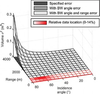
Fig. 11. Single point contribution to mesh-based volume variance (using the Riegl VZ-4000 instrument parameters) versus range and laser-beam incidence angle. At high incidence angles and long ranges the influence of laser beamwidth dominates. The percentages of Montezuma observations falling within the range- and incidence-angle bins used to generate the plot are overlaid (gradient: white (0%) to red (14%)), illustrating that the majority of TLS observations occur at high incidence angles and will make significant contributions to volume variance at longer ranges.
Conclusions
A rigorous method of TLS observation and registration error propagation was demonstrated in order to produce an estimated covariance matrix for each TLS point. In addition to standard error sources, angle and range error induced by beamwidth uncertainty and local terrain morphology was included in the error propagation and shown to have a large influence on propagated point and volume errors. The stability of the TLS instrument is also of primary concern, as corrections derived from inclination sensor readings were unable to fully mitigate the effects of tripod movement during scan acquisition.
Propagated volume errors were found to be negligible when compared to the net snow volumes, which suggests the random errors inherent in TLS measurement techniques are of less importance than the selection of surface model structure (raster or mesh). However, the 3-D point errors do influence volume error in an increasing manner as point densities decrease, indicating that specific areas in a domain with reduced point density demand extra scrutiny. The relationship between surface morphology and point density with respect to propagated volume errors is an avenue for additional research, and validation of the propagated TLS point errors with more precise in situ measurements is also recommended. Finally, volume errors produced from mesh-based surfaces are larger than those from raster-based surfaces for point densities under ∼100 points m−2. This is not unexpected, as the mesh method incorporates both horizontal and vertical point error in the error propagation and therefore better represents estimated volume error.
As the scope of TLS applications continues to expand, the value of an estimated point error feature also grows. Simple visualization of the horizontal and vertical error distribution within a point cloud is a powerful tool to reinforce user awareness of TLS accuracy constraints and to enable data quality assessment. In light of the increasing maximum range capabilities of new lidar instruments, it is important that TLS practitioners appreciate the impact that long ranges and high incidence angles have on estimated horizontal and vertical uncertainties when planning data collection campaigns. For example, it may be desirable to spend more time in the field and collect data from several TLS locations in order to minimize the required ranges or incidence angles, which in turn limit point uncertainty magnitudes. Rigorous TLS point error estimates can also be applied to downstream products or methods that employ TLS points, such as the snow volume error estimates computed in this paper; additional examples include appropriate point weighting for point-cloud registration techniques or point-based model fitting. Rigorous estimated point errors from TLS observations are also relevant when TLS data are used to validate independent topographic measurements of a common area, such as photogrammetric measurements or airborne or satellite laser-scanning observations.
Acknowledgements
The Montezuma lidar data were collected with support from the American Avalanche Association Theo Meiners Research Grant and in collaboration with the Arapahoe Basin Ski Patrol. The Mammoth lidar and snow depth data were provided courtesy of the CRREL/UCSB Eastern Sierra Snow Study Site in cooperation with Mammoth Mountain Ski Area. Support for the first and third authors was provided by the US Army Engineer Research and Development Center Cold Regions Research and Engineering Laboratory (ERDC-CRREL) Remote Sensing/GIS Center of Expertise. The authors also thank Alexander Prokop and an anonymous reviewer for detailed and constructive comments that greatly improved the manuscript.


