

The degree-day model is a parameterization for the melt rate of snow and ice at the surface of an ice sheet or glacier. It is a simple, empirical relation which states that the melt rate is proportional to the surface-air temperature excess above 0°C (e.g. Reference Braithwaite, Olesen and In OerlemansBraithwaite and Olesen, 1989; Reference HockHock, 2003). The physical basis of this and related temperature-based melt- index methods was examined by Reference BraithwaiteBraithwaite (1995).
It was suggested by Reference BraithwaiteBraithwaite (1984) that the number of positive degree-days, PDD, could be calculated from the normal probability distribution around the long-term monthly mean temperatures. A form, which is based on that and is widely used in current ice-dynamic models, was proposed by Reference ReehReeh (1991). It reads
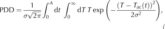
where t is the time, T ac the surface-air temperature, T ac the annual temperature cycle (both in °C) and a the standard deviation of the temperature from the annual cycle, which accounts for the daily cycle and further, stochastic temperature variations. It is often assumed that T ac varies sinusoidally over time,
where T mj is the mean July (January) surface-air temperature on the extratropical Northern (Southern) Hemisphere, T ma is the mean annual surface-air temperature, and A — 1 year. Nonetheless, any other representation of T ac can also be used as a basis for the calculation of the PDD integral (1).
In a number of ice-sheet models (e.g. Reference Huybrechts, Letreguilly and ReehHuybrechts and others, 1991; Reference Van de Wal and OerlemansVan de Wal and Oerlemans, 1997; Reference Tarasov and PeltierTarasov and Peltier, 1999; Reference Marshall, Tarasov, Clarke and PeltierMarshall and others, 2000; Reference Charbit, Ritz and RamsteinCharbit and others, 2002) the double integral in Equation (1) is computed numerically. Since this must be done for each gridpoint separately, it requires a considerable amount of computing time. Further, the inevitable cut-off of the upper limit of the temperature integral at some finite value, T max, influences the accuracy of the results. Therefore, Reference Janssens and HuybrechtsJanssens and Huybrechts (2000) proposed an approximation method for solving the temperature integral by fitting an exponential function.
Here, we demonstrate that the temperature integral can be evaluated fully analytically. To the best of our knowledge, this analytical solution has not been applied to the PDD temperature integral before. A similar procedure was carried out by Reference Roe and LindzenRoe and Lindzen (2001) in the context of determining the precipitation rate over ice sheets. However, they applied an unnecessary absolute value in their equation, they did not show the integration substitutions which lead to the resulting expression and they did not evaluate the integral boundaries of the exponential function. Here, we present the complete derivation and the resulting equations for the temperature integral of the statistical positive degree-day model.
We start by adding the expression
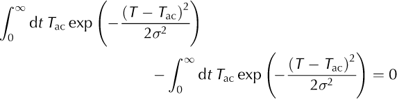
to the temperature integral in Equation (1). This yields
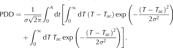
The substitutions ![]() and
and ![]() provide
provide

With the definition of the complementary error function

(e.g. Reference Press, Teukolsky, Vetterling and FlanneryPress and others, 1996, section 6.2; erf(x) denotes the conventional error function) this can be rewritten as
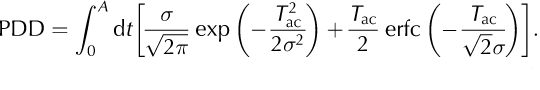
This representation has the great advantage that the temperature integral of the original Equation (1) has vanished. Therefore, it can be numerically evaluated much faster and yields more precise results, because the upper limit i need not be cut off at some finite value. The error function is not a standard built-in function of Fortran 90 or C. However, it is implemented in a number of modern Fortran and C compilers as well as in the packages MATLAB and Mathematica. Alternatively, it can easily be computed by the routines given by Reference Press, Teukolsky, Vetterling and FlanneryPress and others (1996) or similar sources. Here, we employ the subroutine erfcc by Press and others (1996, section 6.2) with a fractional error everywhere less than 1.2✗ 10-7.
We investigate briefly the gain in accuracy and reduction in computing time to solve the new semi-analytical representation for PDD, Equation (6), compared to the fully numerical (Equation (1)) and other representations. Let us consider a typical situation for the ablation zone in south Greenland with T ma = −10°C, T mj = 5°C and σ = 5°C. The time integrals in Equations (1) and (6) are solved with a monthly time-step. In addition, the temperature integral in Equation (1) is computed by the trapezoidal rule with a temperature step of AT = 0.5°C and a cut-off temperature T max varying between 0.5σ and 4σ.

Fig. 1. PDD values and CPU times (109 computations) for the numerical solution of Equation (1) as a function of T max/σ (solid lines) and Equation (6) (dashed lines). For details see main text.
The results are shown in Figure 1. CPU (computing) times refer to computations carried out with a Fortran 90 program, compiled with the Intel Fortran Compiler Version 8 and run on a 3.4GHz Pentium-4 PC under SuSE LINUX 9.0. They are given for 109 computations, which is the approximate number required for a simulation of the Greenland ice sheet with 20 km resolution over 250000years (two glacial- interglacial cycles) with a time-step of 2.5 years. It is evident that our new method of computing the PDD integral is far more efficient than the fully numerical method. In order to be sufficiently accurate, the latter requires at least T max = 3a, and for this cut-off temperature it consumes more than ten times more CPU time than the solution of the semianalytical expression (6).
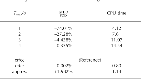
Table 1 gives some more detailed information about the accuracies and CPU times of the different methods. In addition to our representation of the complementary error function by the routine erfcc (Reference Press, Teukolsky, Vetterling and FlanneryPress and others, 1996), we have considered the rational approximation by Abramowitz (1970, section 7.1.25), here denoted as erfcr, which has an absolute error <2.5x10⁻⁵. This approximation was also used by Reference Roe and LindzenRoe and Lindzen (2001), but they did not give the values for the parameters. Further, we have implemented the approximate solution of the temperature integral in Equation (1) by Reference Janssens and HuybrechtsJanssens and Huybrechts (2000) (here called approx). There is only a tiny difference in accuracy between the PDD values resulting from the erfcc and the erfcr representations of the complementary error function. The error due to the numerical integration over the year outweighs the differences in accuracy of the representations of the complementary error function. The accuracy of the approximation by Reference Janssens and HuybrechtsJanssens and Huybrechts (2000) is clearly lower than that of both other methods, but is certainly tolerable in view of the relatively crude assumptions of the positive degree-day method itself (e.g. the approximation of the synoptic processes by the normal probability distribution (Reference BraithwaiteBraithwaite, 1984)). The computing time for the method with erfcc is slightly longer that that with erfcr, because of the higher-order representation of the complementary error function in the former. Interestingly, the approximation by Reference Janssens and HuybrechtsJanssens and Huybrechts (2000) is, at least in our implementation, about 14% slower despite its lower accuracy. This is presumably because three different functions (abs, exp, max) must be evaluated in this approximation.
Since the complementary error function is available in nearly every compiler, or, alternatively, can be easily implemented by several tested subroutines with low computational time and high accuracy, we strongly encourage ice- sheet and glacier modellers to make use of this improved method.
Table 1. Accuracy (with respect to erfcc) and relative CPU time(erfcc = 1) for different methods of solving the PDD integral. Details are given in the main text. See also Figure 1
Epilogue
Reference BraithwaiteBraithwaite’s (1984) introduction of the normal distribution in order to reduce the degree-day calculations to monthly rather than daily data reduced data requirements by a factor of 30. The methods presented in this work save more than 90% computing time. Who is going to make the next saving?
Acknowledgement
We thank R.J. Braithwaite and R.C. Warner for their constructive comments on the original version of this correspondence.


