


Introduction and background
The crystal orientation fabric of ice (or simply fabric) refers to the ensemble of grain c-axis orientations (basal plane normal directions) making up the polycrystal. Ice displays a strong mechanical anisotropy; for an individual grain, shear is ~104 times easier perpendicular to the c-axis than parallel to it (Duval and others, Reference Duval, Ashby and Anderman1983). At the polycrystal scale, grain interactions reduce this effect, but single-maximum fabrics (i.e. polycrystals with a strong alignment of c-axes in one direction) have been found to shear more easily by an order of magnitude compared to isotropic fabrics (Pimienta and Duval, Reference Pimienta and Duval1987). This induced anisotropy can have significant implications for ice flow by localizing shear near the bed (Thorsteinsson, Reference Thorsteinsson2001; Rathmann and Lilien, Reference Rathmann and Lilien2022a) or in the margins of ice streams (Minchew and others, Reference Minchew, Meyer, Robel, Gudmundsson and Simons2018; Grinsted and others, Reference Grinsted2022). Despite the strong effect that fabric can have upon flow, large-scale models of ice flow generally neglect the fabric-induced mechanical anisotropy. In part, the effects are neglected due to unknown fabrics in the dynamic regions where fabric may most affect flow, since challenging conditions have limited direct measurements of fabric in such areas (Jackson and Kamb, Reference Jackson and Kamb1997; Thomas and others, Reference Thomas2021). Active and passive seismics (e.g. Bentley, Reference Bentley1971; Smith and others, Reference Smith2017; Lutz and others, Reference Lutz2022) and phase-sensitive radar (pRES) (e.g. Brisbourne and others, Reference Brisbourne2019; Jordan and others, Reference Jordan, Schroeder, Castelletti, Li and Dall2019) provide some constraints if surface access is possible, though depth resolution and precision are limited. In the fastest flowing regions, new methods have only recently allowed inference of fabric from airborne radar data (Young and others, Reference Young2021), thus allowing the first continuous, spatially extensive inferences of fabric. Models of fabric development can potentially be used to estimate the fabric between sparse measurements, particularly in dynamically interesting areas such as ice streams.
Modeling crystal processes
Fabric-evolution models range from small-scale (sub-meter) models that track individual ice grains to large-scale (kilometer or greater) models that rely on statistical descriptions of fabric (e.g. Gillet-Chaulet and others, Reference Gillet-Chaulet, Gagliardini, Meyssonnier, Zwinger and Ruokolainen2006; Llorens and others, Reference Llorens2016). These models broadly include two processes: deformation that mechanically affects the distribution of grain orientations, a process termed lattice rotation, and mass movement between grains, termed recrystallization.
The effect of lattice rotation (the apparent rotation of c-axes) has been suggested to depend linearly on the deformation gradient (e.g. Svendsen and Hutter, Reference Svendsen and Hutter1996), assuming most deformation occurs as slip on the basal planes. However, this simple form does not apply at the polycrystal scale. The bulk fabric evolution depends on how the bulk stress and strain transfer to the smaller grain scale; though simple assumptions about uniform stress and strain are often used, the reality is more complex than can currently be represented by large-scale models (Castelnau and others, Reference Castelnau, Duval, Lebensohn and Canova1996; Rathmann and Lilien, Reference Rathmann and Lilien2022a). Nevertheless, models of fabric evolution that account for lattice rotation alone, under the assumption of homogeneous strain or stress over the polycrystal scale, are able to do a good job reproducing ice-core measurements in some locations (Gillet-Chaulet and others, Reference Gillet-Chaulet, Gagliardini, Meyssonnier, Zwinger and Ruokolainen2006; Rathmann and Lilien, Reference Rathmann and Lilien2022a), suggesting that this process is well-described at least near ice divides and domes where such ice cores are drilled.
Recrystallization dominates fabric development in some regimes (e.g. Alley, Reference Alley1988), but is generally neglected in large-scale fabric models. Recrystallization encompasses three processes: normal grain growth, rotation recrystallization (also called continuous dynamic recrystallization, or CDRX), and migration recrystallization (also called discontinuous dynamic recrystallization, or DDRX). Normal grain growth refers to the orientation-independent enlargement of grains near the surface of the ice sheet, and does not strongly affect fabric (Montagnat and Duval, Reference Montagnat and Duval2000). Rotation recrystallization refers to the division of grains into subgrains during deformation, and has been found to occur in relatively shallow parts of ice sheets (e.g. Weikusat and others, Reference Weikusat, Kipfstuhl, Faria, Azuma and Miyamoto2009). However, since the new grains are split from their parents gradually, they do not lead to a significantly different preferred orientation, but rather cause a slowing of fabric development (Montagnat and Duval, Reference Montagnat and Duval2000), which is sometimes modeled as a diffusive process on the orientation of the grains (Gödert, Reference Gödert2003; Placidi and others, Reference Placidi, Greve, Seddik and Faria2010; Richards and others, Reference Richards, Pegler, Piazolo and Harlen2021). Migration recrystallization refers to the movement of mass to (possibly new) grains well-oriented for the in situ stress (Chapelle and others, Reference Chapelle, Castelnau, Lipenkov and Duval1998). Though early evidence (Alley, Reference Alley1988; Duval and Castelnau, Reference Duval and Castelnau1995) suggested that migration recrystallization only affects warm ($\ge -10^{\circ}$ C), deep ice, some ice-core evidence has indicated that the process occurs shallower (Diprinzio and others, Reference Diprinzio2005; Kipfstuhl and others, Reference Kipfstuhl2006, Reference Kipfstuhl2009). These observations led to a proposal of a new paradigm for the activation of migration recrystallization at sufficient stress, even if ice is cold (Faria and others, Reference Faria, Weikusat and Azuma2014). The bulk effect of migration recrystallization on fabric can be simulated as a production/decay process that leads to grains well-oriented for the in situ stress or strain rate (Gödert and Hutter, Reference Gödert and Hutter1998; Faria and others, Reference Faria, Kremer and Hutter2003; Placidi and others, Reference Placidi, Greve, Seddik and Faria2010) and the necessary model parameters have recently been tuned to experimental data (Richards and others, Reference Richards, Pegler, Piazolo and Harlen2021).
Current anisotropic ice-flow models
Models of fabric development are, with few exceptions, separate from ice-flow models. Only a few large-scale ice-flow models consider the effect of fabric on flow, let alone track its development explicitly. To the extent that the effect of fabric is included, it is often as a strain-rate enhancement factor, which can be isotropic or anisotropic (i.e. the material response may or may not be invariant to rotations from a reference state) depending on how the scalar factor is calculated (Seddik and others, Reference Seddik, Greve, Placidi, Hamann and Gagliardini2008; Graham and others, Reference Graham, Morlighem, Warner and Treverrow2018). Since, in practice, much ice-flow modeling infers a scalar enhancement factor prior to prognostic simulations (e.g. Larour and others, Reference Larour, Rignot, Joughin and Aubry2005; Arthern and Gudmundsson, Reference Arthern and Gudmundsson2010), the influence of fabric may be subsumed into the bulk viscosity along with other factors causing enhancements, e.g. variations in mechanical damage or temperature. Such scalar compensation may successfully account for the instantaneous effect of anisotropy on strain in the dominant direction (Rathmann and Lilien, Reference Rathmann and Lilien2022a), but by definition cannot accurately describe the viscosity in all directions; if conditions change or if multiple deformation modes are active, scalar compensation may lead to incorrect transient results.
Other models account for anisotropy by assuming that fabric adjusts instantaneously to the steady state fabric pattern consistent with in situ stress and strain (Graham and others, Reference Graham, Morlighem, Warner and Treverrow2018), and thus obviate the need for a time-evolving fabric model. However, this assumption is poorly supported for many parts of ice-sheet interiors, where fabric is thought to develop slowly by lattice rotation (Alley, Reference Alley1988). For example, the stress state is unconfined compression at all depths beneath a perfect dome, but fabric varies from isotropic at the surface to a single maximum at depth (e.g. Durand and others, Reference Durand2009). To determine fabric accurately everywhere, lattice rotation and recrystallization must both be accounted for, which necessitates a model of fabric development that includes transient and advective effects (e.g. Thorsteinsson and others, Reference Thorsteinsson, Waddington and Fletcher2003).
Finally, one large-scale model, Elmer/Ice, is capable of simulating fabric evolution explicitly and couples that evolution to flow (Gillet-Chaulet and others, Reference Gillet-Chaulet, Gagliardini, Meyssonnier, Zwinger and Ruokolainen2006; Seddik and others, Reference Seddik, Greve, Placidi, Hamann and Gagliardini2008). In that module, fabric is assumed to develop solely due to lattice rotation, and the closure approximation, which relieves the need to track infinitely detailed information about fabric orientation, contains implicit site-specific tuning; the effect of this closure approximation is essentially untested due to the lack of closure-approximation-free model for comparison. The fabric evolution module is not commonly used despite the widespread applications of Elmer/Ice. This limited use stems from the added computational cost of simulating the fabric, more free model parameters typically unconstrained by observations, and violation of the lattice-rotation-only assumption in fast-flowing areas where the ice-flow model is most commonly applied.
Fabric representation
To model fabric development and its effect on bulk directional ice viscosities, a mathematical description of grain orientations is needed. A full description of the fabric would contain information about the orientation, size, shape and number of grains that makes up the polycrystal, properties that can be simulated explicitly using small (sub-meter scale) microstructural models (e.g. Durand, Reference Durand2004). In practice, large-scale fabric models generally ignore the size and shape of grains, and explicitly track the orientation alone (Gillet-Chaulet and others, Reference Gillet-Chaulet, Gagliardini, Meyssonnier, Zwinger and Ruokolainen2006; Seddik and others, Reference Seddik, Greve, Placidi, Hamann and Gagliardini2008; Richards and others, Reference Richards, Pegler, Piazolo and Harlen2021). Large-scale models of fabric development rely on the distribution of preferred grain orientations in order to construct grain-weighted-average quantities such as directional viscosities (e.g. Rathmann and Lilien, Reference Rathmann and Lilien2022b). Different weights can be used to construct average quantities, such as the distribution of number of grains or their mass in orientation space, S 2 (surface of the unit sphere).
Orientation distribution functions
In the simplest approach, the orientation distribution gives equal weight to all grains, defined as the orientation distribution function (ODF):

where ψ is the c-axis orientation density, θ and ϕ are the polar and azimuth angles, respectively, $N = \int _{S^2} \psi \, {\rm d}\Omega$ is the total number of grains and the differential of the solid angle is dΩ = sin (θ) dθ dϕ.
An alternative orientation distribution may be defined by regarding the grain mass density as a function of orientation, ϱ*(θ, ϕ), termed the orientation mass density, a concept that arises from the theory of mixtures of continuous diversity (Faria, Reference Faria2001). By analogy to the ODF, we define a mass orientation distribution function (MODF), which is ϱ* normalized:

where $\rho _{\rm i} = \int _{S^2}\varrho ^\ast \, {\rm d}\Omega$ is simply the density of ice.
Structure tensors and closure
An arbitrary (M)ODF will not necessarily have a closed form, so large-scale models have previously proposed several mathematical representations of fabric, perhaps the simplest of which is the cone- and girdle-angle model (e.g. Thorsteinsson, Reference Thorsteinsson2001). More complex models have relied on the fact that any (M)ODF can be expanded in terms of a structure-tensor series (e.g. Svendsen and Hutter, Reference Svendsen and Hutter1996), useful for directly calculating bulk directional viscosities. The structure tensors are the moments of the fabric orientation distribution, defined as the sum of the weighted m-fold outer product of grain c-axes with themselves. For a discrete set of N grains with c-axis denoted ci, it is defined as

where (ci ⊗ )m is the m-repeated outer product, and m is the (even) order of the tensor (Advani and Tucker, Reference Advani and Tucker1987). The weights w i are normalized such that $\sum _i^N w_i = 1$ . If no shape/size information is available, then all grains are typically weighted equally (w i = 1/N) so (3) becomes the arithmetic mean, and the a(m) are moments of the ODF. If the w i are taken to be the volume or mass fraction (i.e. the MODF itself), then the a(m) are the moments of the MODF.
In practice, the structure-tensor series representation of fabric is often truncated at the second-order contribution a(2) (i.e. excluding a(m) for m > 2) (Gillet-Chaulet and others, Reference Gillet-Chaulet, Gagliardini, Meyssonnier, Zwinger and Ruokolainen2006; Seddik and others, Reference Seddik, Greve, Placidi, Hamann and Gagliardini2008). a(2) alone is sufficient to represent simple yet common fabrics such as single-maximum and girdle fabrics found in deep ice cores (Gow and Williamson, Reference Gow and Williamson1976; Advani and Tucker, Reference Advani and Tucker1987; Weikusat and others, Reference Weikusat2017; Bauer and Böhlke, Reference Bauer and Böhlke2021). Such ice-core measurements often discard (or cannot recover) the principal directions and retain only the eigenvalues of a(2), here ordered such that λ 3 ≥ λ 2 ≥ λ 1 (though conventions differ).
Complicated fabrics that cannot be expressed in terms of a(2) alone have also been observed. For example, ice cores from dynamic areas (Jackson and Kamb, Reference Jackson and Kamb1997; Gerbi and others, Reference Gerbi2021) and laboratory experiments (Journaux and others, Reference Journaux2019; Fan and others, Reference Fan2020) show multi-maxima and ‘diamond’ fabrics; a(2) cannot capture such structure. Tracking higher-order structure tensors would allow more complex fabrics to be modeled, but this quickly becomes challenging for technical reasons, including degeneracy of the tensors (e.g. the information contained in a(2) is included in a(4); Bauer and Böhlke, Reference Bauer and Böhlke2021), complications of tracking moments of the fabric rather than the fabric itself, and the lack of closure for lattice rotation (the evolution of a(2) depends on a(4), that of a(4) on a(6), etc.).
Expansion series approach
Some of the issues of the structure-tensor approach can be avoided by describing the fabric as a series of increasingly finer anomalies from isotropy in spectral space. Richards and others (Reference Richards, Pegler, Piazolo and Harlen2021) and Rathmann and others (Reference Rathmann, Hvidberg, Grinsted, Lilien and Dahl-Jensen2021) independently proposed using a spherical harmonic expansion of ϱ* or ψ for polycrystalline viscoplastic problems. This approach has long been used for elastic problems (Turner, Reference Turner1999), but is new to glaciology. In this formulation, an arbitrary ϱ* can be described by a harmonic series expansion

where L is the order of the approximation (spectral truncation), $\hat \varrho _{l}^{m}$ are the complex expansion coefficients and $Y_{l}^{m}$
 the spherical harmonic functions. Since ϱ* is antipodally symmetric, $\hat \varrho _l^m = 0$
 if l is odd. This approach describes the MODF (ϱ*/ρ i) directly, without parameterization and has recently been applied to model individual ice parcels (Rathmann and others, Reference Rathmann, Hvidberg, Grinsted, Lilien and Dahl-Jensen2021; Richards and others, Reference Richards, Pegler, Piazolo and Harlen2021) and to a simplified, slab model of ice flow (Rathmann and Lilien, Reference Rathmann and Lilien2022a).
Physical and technical advantages are discussed below. Here, it is sufficient to note that, for a given L, expansion (4) contains the same information as structure tensors up to order L (Rathmann and others, Reference Rathmann, Hvidberg, Grinsted, Lilien and Dahl-Jensen2021).
Modeling the ODF or MODF
Here, like Richards and others (Reference Richards, Pegler, Piazolo and Harlen2021), we consider ϱ*, since it provides a framework where recrystallization can naturally be modeled as the transfer of mass between grains with different orientations. Indeed, when recrystallization is active, the total number of grains is not conserved (i.e. ∂N/∂t ≠ 0) unlike total mass (per unit volume). However, Rathmann and Lilien (Reference Rathmann and Lilien2022a) proposed using the same DDRX model math for representing the effect on the ODF, in which case grains (orientations) are understood to spontaneously decay and nucleate in equal proportion so that N is conserved. Since, ψ and ϱ* are mathematically identical up to their normalization in these two models, the MODF and ODF are identical, and hence modeled a(m), too, although by formulating the model in terms of ϱ* it rests on stronger physical grounds.
Motivation: the need for a higher-order model
In this work, we adopt the spherical harmonic expansion of ϱ*, allowing arbitrary grain orientation distributions to be represented. Before proceeding, we demonstrate that such an approach is necessary because the existing structure-tensor-based representations (and closure schemes) are inadequate for modeling migration recrystallization. Although such models are usually formulated in terms of the ODF, the limitations described next would persist even if the models were reinterpreted in terms of the MODF.
When lattice rotation dominates fabric evolution, the evolution of a(2) can be written in closed form by parameterizing a(4) in terms of a(2). Figure 1 makes this clear, showing the relationship between the unique lowest-order expansion coefficients of the MODF, $\hat \varrho _2^0$ and $\hat \varrho _4^0$
 , derived from ice cores and lab experiments (shown by hollow markers), in a frame where fabric is approximately rotationally symmetry around the vertical axis (by first rotating the fabric before comparison, no generality is lost by considering such a reference frame). Since the corresponding unique lowest-order tensorial components are linearly related to $\hat \varrho _2^0$
 and $\hat \varrho _4^0$
 , a tensorial correlation between a(4) and a(2) likewise exists. Gillet-Chaulet and others (Reference Gillet-Chaulet, Gagliardini, Meyssonnier, Montagnat and Castelnau2005) noted this by considering an analytical model of fabric development, for multiple types of deformation, leading to the tensorial closure function a(4)(a(2)) currently used by Elmer/Ice's anisotropic flow solver. Indeed, the colored lines in Figure 1 show that a zero-dimensional model (Rathmann and others, Reference Rathmann, Hvidberg, Grinsted, Lilien and Dahl-Jensen2021) considering only lattice rotation produces a single consistent relationship between second- and fourth-order terms of the fabric under simple shear, unconfined extension or unconfined compression, confirming that there is a function a(4)(a(2)) that applies regardless of the type of deformation. Thus, if one is concerned only with the evolution of second-order moments of the fabric under lattice rotation, the closure approximation of Gillet-Chaulet and others (Reference Gillet-Chaulet, Gagliardini, Meyssonnier, Montagnat and Castelnau2005) is sufficient and higher-order fabric representations provide little benefit.

Figure 1. Relationship between normalized expansion coefficients $\hat \varrho _2^0/\hat \varrho _0^0$ and $\hat \varrho _4^0/\hat \varrho _0^0$
 in zero-dimensional modeling (lines) and from observations (markers). All fabric states are rotated into a (nearly) vertically symmetric reference frame. The two components fully capture the second- and fourth-order fabric strength in the case of vertical symmetry, where the white/colored region represents the space of possible fabric states (MODFs) with a vertical symmetry. Lines show modeled fabric evolution using SpecFab (Rathmann and others, Reference Rathmann, Hvidberg, Grinsted, Lilien and Dahl-Jensen2021) with lattice rotation alone (brown/green) and with DDRX alone (red). Increasing the strength of recrystallization causes greater deviation from the lattice rotation trajectories, eventually resulting in a steady relationship between $\hat \varrho _2^0$
 and $\hat \varrho _4^0$
 regardless of deformation amount (solid red circle). Hollow markers show fabrics observed in the laboratory and in ice cores. The marker shape indicates the deformation regime: triangles for extension, diamonds and crosses for compression and squares for simple shear. Color indicates source for each dataset: blue from Thorsteinsson and others (Reference Thorsteinsson, Kipfstuhl and Miller1997), pink from Treverrow and others (Reference Treverrow, Jun and Jacka2016), purple from Westhoff and others (Reference Westhoff2021), orange from Voigt (Reference Voigt2017), green from Thomas and others (Reference Thomas2021) and yellow from Qi and others (Reference Qi2019). Crosses indicate DDRX-affected fabrics during relatively warm deformation tests: red markers from Fan and others (Reference Fan2020), and gray markers from Hunter and others (Reference Hunter, Wilson and Luzin2023). Ball plots show the corresponding MODFs at different points in the state space. Gray contours show modeled enhancement factors for vertical compression/extension, E zz. Any vertical spread in observations at a single $\hat \varrho _2^0/\hat \varrho _0^0$
 cannot be captured by a traditional closure approximation.
Migration recrystallization makes the correlation function multi-valued, preventing use of a closure approximation. Figure 1 demonstrates this, showing that DDRX-affected fabrics measured in the lab (red and gray markers) and an existing DDRX model (red lines) cause fabric-state trajectories to diverge from the approximate correlation found for lattice-rotation-induced fabrics. Hence, $\hat \varrho _4^0$ is not always uniquely defined by $\hat \varrho _2^0$
 (or a(4) by a(2)). Thus, since the evolution of a(2) depends on a(4), a(4) must be allowed to freely evolve, too, when migration recrystallization is active.
To some degree, the spread in fabric observed in laboratory and ice-core data suggests that the effect of recrystallization is always present (Fig. 1). These data thus suggest that migration recrystallization should always be included in fabric-evolution models, even if lattice rotation is the primary control on fabric development in many areas. Including this effect is particularly important for understanding the implications of the fabric upon ice flow, since the directional viscosities are thought to depend on both a(2) and a(4) (e.g. Gillet-Chaulet and others, Reference Gillet-Chaulet, Gagliardini, Meyssonnier, Zwinger and Ruokolainen2006; Rathmann and Lilien, Reference Rathmann and Lilien2022b). The gray contours in Figure 1 show the modeled compressional/extensional enhancement factor, E zz, along the z-axis (the viscosity model is introduced below), indicating fabric-induced hardness may be overestimated by $\sim \! 40\%$ if DDRX is active (red and gray markers) but a correlation based on lattice rotation is assumed (green model line). In such a case, using a model of fabric development to constrain directional viscosity is only useful if the model considers migration recrystallization as well as lattice rotation; otherwise, an isotropic ice-flow model has similar error.
Including fourth-order terms, and consequently modeling recrystallization, requires either including higher-order tensors in structure-tensor-based models, and thus a closure approximation of a(4) in terms of a(6) or a similar higher-order closure, or a switch to another approach. Here, we incorporate the above spectral description of fabric as a new module in Elmer/Ice (Zwinger and others, Reference Zwinger, Greve, Gagliardini, Shiraiwa and Lyly2007; Gagliardini and others, Reference Gagliardini2013), a state-of-the-art ice-flow model, providing an alternative to the current structure-tensor-based fabric representation. In coupling to flow, we also implement the recently derived, unapproximated nonlinear orthotropic rheology, validated against Dye-3 deformation tests (Rathmann and Lilien, Reference Rathmann and Lilien2022b), which is expected to be important when fabric and stress are misaligned.
We consider a higher-order approximation of the fabric (L = 6, but not limited thereto), and model the (transient) effect of both lattice rotation and migration recrystallization on large-scale fabric development and ice flow, while removing any closure approximations and resulting error in the viscosity. Using rates of rotation and migration recrystallization tuned to laboratory measurements and ice-core data, we apply the new nonlinear, tensorially anisotropic, thermally coupled ice-flow model to a realistic geometry. While the added complexity of this model is most relevant for more dynamic areas, the dearth of data prevents meaningful validation in such regions. Instead, we model a transect across Dome C, East Antarctica and compare to ice-core (Durand and others, Reference Durand2009) and phase-sensitive radar (Corr and others, Reference Corr, Ritz and Martin2021; Ershadi and others, Reference Ershadi2022) measurements of fabric there.
Notation
Throughout, bold symbols indicate tensors and vectors. The operator $\nabla _{S^2}$ denotes the gradient in orientation space (S 2), while $\nabla$
 is the gradient in Cartesian space. The subscript g denotes a grain parameter. Other operators follow standard conventions; a full list of symbols is given in Table 1.
Table 1. Notation used in the text

Model
We are interested in modeling fabric development and its effect upon ice flow. This is a coupled problem since the fabric evolution depends on the stress and strain rates, and vice versa. Moreover, since recrystallization and the isotropic part of the viscosity are temperature dependent, the temperature field must be simulated or specified. Finally, the ice geometry (i.e. a free surface) must be updated based on mass conservation. We first present the model equations, then describe the application to Dome C.
Fabric model
We account for the combined effects of lattice rotation, migration recrystallization and rotation recrystallization in a single model of fabric development. Specifically, we follow Placidi and others (Reference Placidi, Greve, Seddik and Faria2010); Rathmann and Lilien (Reference Rathmann and Lilien2022a) and Richards and others (Reference Richards, Pegler, Piazolo and Harlen2021) by modeling the rate-of-change of ϱ*(x, t, θ, ϕ) as

where

is the material derivative, u(x, t) is the bulk velocity, $\dot {{\boldsymbol c}}( \theta ,\; \, \phi ,\; \, {\boldsymbol u})$ is the rate-of-change in orientation of an individual c-axis due to lattice rotation (c-axis angular velocity field on S 2), Γ(θ, ϕ, τ) is an orientation-dependent mass production/loss rate describing the effect of migration recrystallization given the deviatoric stress tensor τ and Λ0 is the scalar rate of rotation recrystallization. We address each of these terms in turn.
Lattice rotation
Let ${\dot {\boldsymbol \epsilon }} = ( \nabla {\boldsymbol u} + \nabla {\boldsymbol u}^{\intercal} ) / 2$ be the bulk strain-rate tensor, and ${\boldsymbol W} = ( \nabla {\boldsymbol u} - \nabla {\boldsymbol u}^{\intercal} ) / 2$
 the bulk spin tensor. If lattice rotation is regarded as a kinematic process (i.e. grains reorient passively), the apparent rotation of an individual c-axis can be modeled as

where c = [sin (θ)cos (ϕ), sin (θ)sin (ϕ), cos (θ)], ${\dot {\boldsymbol \epsilon }}_{\rm g}$ is the strain rate at the grain scale, and $\iota$
 is a parameter determining the ratio of basal slip to rigid body rotation (e.g. Svendsen and Hutter, Reference Svendsen and Hutter1996). As discussed in the section on calibration below, we take $\iota = 1$
 , equivalent to assuming that the deformation in simple shear behaves like a deck of cards (following, e.g. Gagliardini and Meyssonnier, Reference Gagliardini and Meyssonnier1999). In practice, only ${\dot {\boldsymbol \epsilon }}$
 is known/computed, while individual grains are subject to a heterogeneous strain-rate field, ${{\dot {\boldsymbol \epsilon }}}_{\rm g}$
 , where ${{\dot {\boldsymbol \epsilon }}}_{\rm g} = {\dot {\boldsymbol \epsilon }}$
 is not guaranteed. This heterogeneity is not easily modeled, so two assumptions are common: the Sachs hypothesis, that stress is homogeneous, and the Taylor hypothesis, that the strain rate is homogeneous. Here, we use an intermediate approximation following Gillet-Chaulet and others (Reference Gillet-Chaulet, Gagliardini, Meyssonnier, Zwinger and Ruokolainen2006), namely

where α LR ∈ [0; 1] is an interaction parameter dictating the compromise between the Taylor and Sachs hypotheses and η 0 is the nonlinear viscosity (defined in Eqn (18)). We take α LR = 0.06 following previous work (Ma and others, Reference Ma2010; Lilien and others, Reference Lilien, Rathmann, Hvidberg and Dahl-Jensen2021), though we expect the results to be insensitive to this choice for α LR < 0.1 (Martín and others, Reference Martín, Gudmundsson, Pritchard and Gagliardini2009).
Migration recrystallization
Migration recrystallization is modeled as an orientation-dependent production/decay process proportional to the square of the shear stress resolved on basal planes, similar to Placidi and others (Reference Placidi, Greve, Seddik and Faria2010). In effect, this parameterization compares the fabric state to the state most favorable for deformation, causing the MODF to decrease in directions that are unfavorable (little basal-plane resolved shear stress) and increase in favorable directions (high basal-plane resolved shear stress). The production/decay rate, Γ, is taken to be

where Γ0 is a rate factor, and the deformability, D, is given by (Placidi and others, Reference Placidi, Greve, Seddik and Faria2010; Richards and others, Reference Richards, Pegler, Piazolo and Harlen2021)

D describes the favorable/unfavorable c-axis directions and is dictated solely by the stress, while 〈D〉 describes how favorably the current fabric configuration is, which depends on the local second- and fourth-order structure tensors and τ.
This formulation differs slightly from previous work (Placidi and others, Reference Placidi, Greve, Seddik and Faria2010; Richards and others, Reference Richards, Pegler, Piazolo and Harlen2021) by using the stress tensor, rather than the strain-rate tensor, to determine the deformability (and thus the directions in which grain growth occurs). This is simply an alternative parameterization of the underlying process, which is thought to depend on a number of microphysical parameters including dislocation density in addition to τ and ${\dot {\boldsymbol \epsilon }}$ (Faria, Reference Faria2006a, Reference Faria2006b). Since previous work considered a scalar viscosity, τ and ${\dot {\boldsymbol \epsilon }}$
 were co-axial, and hence using either in Eqn (10) was equivalent. Because migration recrystallization is thought to depend on stress rather than the strain rate (e.g. Duval and Castelnau, Reference Duval and Castelnau1995; Chapelle and others, Reference Chapelle, Castelnau, Lipenkov and Duval1998), the distinction is relevant when coaxiality cannot be assumed, such as is the case for the bulk flow law we introduce below. However, we note that while the using τ versus ${\dot {\boldsymbol \epsilon }}$
 in Eqn (10) will have an effect on the fabric development, neither choice is superior to the other, and a more complete treatment would likely require a full microstructural model (e.g. Faria, Reference Faria2006b).
Finally, we are left to determine an overall rate for this process. While the rate as well as the direction in orientation space of migration recrystallization is thought to depend on several microphysical properties (Faria, Reference Faria2006a, Reference Faria2006b), we retain the assumption of previous work (Richards and others, Reference Richards, Pegler, Piazolo and Harlen2021) that the total amount of recrystallization is related only to the total strain, not rate or stress at which the strain occurred. We thus parameterize the overall rate factor as

where $A_\Gamma$ and $Q_\Gamma$
 are tunable parameters, ${{\dot {\epsilon }}}_{\rm E}$
 is the effective strain rate and R is the universal gas constant. This differs slightly from Richards and others (Reference Richards, Pegler, Piazolo and Harlen2021), which used a linear dependence on temperature, based upon laboratory experiments, while we use an Arrhenius relationship based on ice-core data indicating rapid activation above $-10^\circ$
 C (Alley, Reference Alley1988; Duval and Castelnau, Reference Duval and Castelnau1995). The Arrhenius activation is used to make the model applicable closer to the melting point; within the regime of temperatures considered by Richards and others (Reference Richards, Pegler, Piazolo and Harlen2021), the Arrhenius relationship is close to linear and the approaches are essentially equivalent.
Rotation recrystallization
Rotation recrystallization is modeled as a diffusive process in orientation space (Placidi and others, Reference Placidi, Greve, Seddik and Faria2010) with diffusion coefficient (or rate factor) Λ0. This is a phenomenological description, consistent with the definition of rotation recrystallization in that new grains are created by splitting off from parent grains with similar orientations. Since ice-core evidence indicates a gradual activation of rotation recrystallization compared to migration recrystallization, we follow Richards and others (Reference Richards, Pegler, Piazolo and Harlen2021) exactly by setting

where $m_\Lambda$ and $b_\Lambda$
 are the slope and intercept of the temperature relationship.
Fabric numerics
Numerically, we represent ϱ* using the spectral expansion in Eqn (4) with L = 6, leading to 28 $\hat \varrho _l^m\in {\opf C}$ . The problem is solved on a finite-element mesh, in two or three dimensions. The model mesh is Eulerian, so the fabric evolution has an advective component (last term in Eqn (6)) and a reactive component (right-hand side of Eqn (5)). In our implementation, these two contributions are handled separately. Dϱ*/Dt at each node is determined from the current fabric state, ϱ*, using the SpecFab code of Rathmann and Lilien (Reference Rathmann and Lilien2022a). The advective term is handled using the existing code in Elmer/Ice with using residual-free bubble elements for stabilization.
We treat the real and imaginary components of $\hat \varrho _l^m$ separately, leading to 56 values to track per computational node. However, not all coefficients are independent; we leverage the Hermitian (anti)symmetry of the spectral expansion

which allows direct calculation of the coefficients m < 0 from those with m > 0. Moreover, the fabric model (Eqn (5)) conserves mass, and we assume incompressibility, so ρ i is constant and thus $\hat \varrho ^0_0$ is constant as well since $\rho _{\rm i} = \sqrt {4\pi }\hat \varrho ^0_0$
 . Taking the above considerations into account, 27 unique coefficients are left (though this discussion focuses on L = 6, our Elmer/Ice implementation automatically handles arbitrary L while only computing the unique, independent components). Finally, when ∂u/∂y = 0 (generally equivalent to when the domain is two dimensional (2-D)), a further 12 components are identically zero (although this does not mean that the fabric is 2-D, only that it has useful symmetries, which cause some coefficients to be null). Thus, for L = 6, there are 15 fabric components to consider in 2-D and 27 in three-dimensional (3-D).
Fabric evolution is determined using an implicit timestepping scheme, iterating coefficient-wise. The key difference compared to small-scale spectral models (Rathmann and others, Reference Rathmann, Hvidberg, Grinsted, Lilien and Dahl-Jensen2021; Richards and others, Reference Richards, Pegler, Piazolo and Harlen2021) is that advection greatly increases the problem dimension. That issue is manifest most strongly in 3-D, where a large number of coefficients, combined with many neighbors for a node in the mesh, means that the matrix problem to be solved has a prohibitively wide bandwidth if all fabric coefficients are solved for simultaneously. In order to set up a scheme that would allow an arbitrary L, we thus found it necessary to use a coefficient-wise solution similar to the existing structure-tensor-based fabric module in Elmer/Ice (Gillet-Chaulet and others, Reference Gillet-Chaulet, Gagliardini, Meyssonnier, Zwinger and Ruokolainen2006).
We find that artificial diffusion is necessary in both orientation space (when lattice rotation is active) and in Cartesian space (when migration recrystallization is active) to regularize the problem. For stabilization in orientation space, we use hyper diffusion, which reduces noise in higher-order harmonics while having less effect on lower-order coefficients; the diffusion coefficients were tuned for L = 6 so that, in the steady state, $\hat \varrho _2^m$ are unaffected, whereas $\hat \varrho _4^m$
 are up to 40% smaller compared to L ≥ 20 when subject to unconfined compression. How this affects the ability to simulate strong single maxima, thus limiting the magnitude of simulated bulk directional enhancement factors, is treated in Appendix A. For the stabilization in Cartesian space, we introduce a diffusion term of the form $\zeta _0\nabla ^2\hat \varrho _l^m$
 , where ζ 0 = 5.0 × 10⁻³ a−1 m−1, to the left-hand side of Eqn (5). In theory, this diffusion limits the maximum spatial gradient in fabric, but since fabric transitions slowly this is not a problem in practice; the term only serves to prevent numerical noise in near-zero coefficients from growing during long simulations. Demonstrations of fabric evolution in simple cases, and comparison to existing models, are shown in Appendix A.
Calibration of model parameters
Before applying the model, it is necessary to constrain the rate factors for migration and rotation recrystallization. In order to evaluate the suitability of different rate factors, we compare the fabric predicted by a simplified zero-dimensional model with that observed in the EPICA Dome C (EDC) core (Durand and others, Reference Durand2009). In this calibration, the core was assumed to be drilled at a perfect dome (undergoing unconfined compression), with constant pure shear from surface to bed (i.e. a Nye model of dome strain; Nye, Reference Nye1963). We assumed steady state, so that the fabric evolution of a single, zero-dimensional ice parcel at increasing depth gives the modeled fabric profile of the core. At the surface, the downward velocity was set to be 1.53 cm a−1, the mean accumulation throughout the ice core (Bazin and others, Reference Bazin2013), with zero velocity at the bed. Borehole temperature measurements were used to determine T in order to calculate Λ0 and Γ0 (Buizert and others, Reference Buizert2021). The fabric was assumed to be a weak single maximum with $a^{( 2) }_{zz} = 0.44$ at 214 m depth, matching the first measurement of EDC (Durand and others, Reference Durand2009). Below, fabric evolution followed Eqn (5), under the assumption that the stress and strain are coaxial so that migration recrystallization can be modeled without knowing the rheology. For this purpose, we must assume that α LR = 0 (i.e. the Taylor hypothesis), since τ cannot be calculated in this zero-dimensional model. The model was implemented purely using SpecFab (Rathmann and others, Reference Rathmann, Hvidberg, Grinsted, Lilien and Dahl-Jensen2021), and solved for all complex fabric coefficients simultaneously using forward-Euler timestepping with 200–3200 year time steps.
For evaluation, the modeled fabric was compared to fabric measured on vertical thin sections cut every 11–50 m along the EDC core (Durand and others, Reference Durand2009). Although the orientation of the core and therefore the thin sections are unknown, we can still compare the three fabric eigenvalues and identify the vertical component. Moreover, for this simple model, the two horizontal eigenvalues are equal, so there is no need to identify the orientation of the core. For this comparison, we assume that the ODF and MODF are equivalent, i.e. that the grain size distribution is independent of c-axis direction.
We consider two sets of model parameters: one tuned to laboratory data and one to ice-core data (Fig. 2). For the ‘laboratory’ values, we calibrated to the same data as Richards and others (Reference Richards, Pegler, Piazolo and Harlen2021), and used their calibrated Λ0 = 0.001 × T + 0.21, but took $\iota = 1$ , and assumed that Γ0 is defined by Eqn 11. To find $A_\Gamma$
 and $Q_\Gamma$
 , the parameters for this relationship, we used the observations from Richards and others (Reference Richards, Pegler, Piazolo and Harlen2021), Table 1, but fit an exponential relationship rather than a linear one. The resulting values are $A_\Gamma = 1.91\times 10^7$
 and $Q_\Gamma = 3.36\times 10^{4}$
 J mol−1. This set of parameters leads to an RMSE of 0.19 (27% error) in the largest eigenvalue compared to observations (Fig. 2, full blue line). Next, again assuming $\iota = 1$
 , we found a set of ‘ice-core’-calibrated parameters by brute-force optimizing $b_\Lambda$
 and $A_\Gamma$
 to minimize the misfit to the EDC data. To do so, we assumed that the temperature dependence of rotation and migration recrystallization are accurately described by the laboratory-calibrated dependencies (i.e. $m_\Lambda = 1.26\times 10^{-3}$
 ($^\circ$
 C)−1 and $Q_\Gamma = 3.36\times 10^{4\circ }$
 as above). A 2-D grid of values for $b_\Lambda$
 and $A_\Gamma$
 was then explored, first varying by orders of magnitude around the laboratory values and subsequently refining once the order of magnitude was determined. We note that, in this scheme, if $b_\Lambda$
 was small, Λ0 could be negative; since this is physically implausible, Λ0 was assumed to be zero under such conditions. The optimized value for $A_\Gamma$
 was $A_\Gamma = 4.3\times 10^7$
 , which is of the same order as the laboratory-derived value. The optimal value of $b_\Lambda$
 , however, was 0.02, leading to Λ0 being 0 in the top 1000 m and negligible below that. Physically, rotation recrystallization is thought to be most important in the upper portions of the ice sheet, so the parameterization makes little sense with this recalibrated value. For the ‘ice-core’-calibrated parameters, we thus took Λ0 = 0. These parameters led to an RMSE of 0.08 in the largest eigenvalue (11% misfit; dashed blue line in Fig. 2), substantially better than that from the laboratory-calibrated values. Moreover, this misfit was highest near the bottom of the ice core, where substantial spread in the measurements prevents better fitting (Fig. 2).

Figure 2. Rate factor calibration. (a) Modeled eigenvalues, using a zero-dimensional model, resulting from different rate factors. Colors indicate eigenvalue number (blue for λ 3, orange for λ 2 and green for λ 1). Squares show measured fabric (Durand and others, Reference Durand2009). Lines show modeled fabric, using the zero-dimensional model, with lab-calibrated, ice-core-calibrated and Richards and others (Reference Richards, Pegler, Piazolo and Harlen2021) (R2021) parameters indicated by the solid, dashed and dotted lines, respectively. (b) Temperature in the EDC borehole, from Buizert and others (Reference Buizert2021).
For completeness, we also modeled the ice-core fabric using the calibration provided by Richards and others (Reference Richards, Pegler, Piazolo and Harlen2021) without modification: $\iota = 0.026\times T + 1.95$ , Λ0 = 0.001 × T + 0.21, and Γ0 = 0.176 × T + 6.09. This leads to an RMSE of 0.18 in the largest eigenvalue (27% error; dotted blue line in Fig. 2), similar to using the ‘laboratory’ calibration. The difference between this and our ‘laboratory’ calibration stems almost exclusively from the difference in $\iota$
 ; the exponential dependence of Γ0 on temperature has a relatively minor effect. This third set of parameters was not used for large-scale modeling, since it did not produce a good fit to the data and our implementation of the large-scale model assumes $\iota = 1$
 .
.
In addition to the calibration discussed above, we tested sensitivity to three alternative calibration schemes: one restricting the depths at which the model was tuned to <3000 m and two using a Dansgaard–Johnsen model of strain (Dansgaard and Johnsen, Reference Dansgaard and Johnsen1969) rather than a Nye model, also tuned to data <3000 m depth. The restriction in depth avoids possible issues due to a non-dome-like stress state that arguably exists near the bed beneath Dome C (Durand and others, Reference Durand2007). The Dansgaard–Johnsen model uses a somewhat more realistic description of deformation beneath the divide (specifically that the strain rate goes linearly to zero below a certain depth, dubbed the ‘kink height’). Since the height of the kink is poorly constrained, we tested both 0.2 and 0.4 times the ice thickness. Restricting calibration to shallow depths resulted very similar misfit in those depths to the full-depth inference, and rate factors differed by <$5\%$ . With either kink height, the Dansgaard–Johnsen model resulted in a smaller model-data misfit ($\sim \!7\%$
 ) than the Nye model, but the inferred parameters did not differ significantly from those obtained using the Nye model (difference of $< \!5\%$
 ). The results of the additional calibrations are shown in Supplementary Figure S1. While there may be benefits to using one of these alternative calibrations, the full-depth Nye calibration arguably relies on the fewest assumptions, and thus it is what we use in subsequent simulations.
Ice flow
Ice flow is an incompressible Stokes flow

governed by the momentum balance

where u is the bulk velocity, σ is the Cauchy stress tensor, ρ i the density of ice and g the gravity vector.
For a constitutive relation, we adopt an unapproximated nonlinear extension of the orthotropic flow law (Rathmann and Lilien, Reference Rathmann and Lilien2022b), which, following plastic potential theory, has a nonlinear viscosity that depends on all orthotropic strain-rate tensor invariants:

where the mi's are the three reflection-symmetry directions that the fabric is presumed to have (taken to be coincident with the eigenvectors of a(2)).
Posed in inverse form (i.e. the deviatoric stress as a function of strain rate) the constitutive relation is

where j = (2, 3, 1) and k = (3, 1, 2) are index variables, I is the identity and the nonlinear, isotropic part of the viscosity is

where n is the flow law exponent (taken to be the canonical n = 3). Let

then the six dimensionless, relative directional viscosities are (for i = 1, 2, 3)


which depend on the eigenenhancements, E ij, defined as the bulk directional enhancement factors (induced by fabric) in the directions of the fabric symmetry axes, mi.
Directional enhancement factors
We are left to provide a mechanism to calculate the directional enhancement factors induced by an anisotropic fabric, defined as

where ${\dot {\boldsymbol \epsilon }}$ is the corresponding forward form of Eqn (17), ${\dot {\boldsymbol \epsilon }}_{\rm iso}$
 is the strain-rate assuming isotropy (ϱ* = const.), and

are idealized longitudinal (i = j) and shear (i ≠ j) stress-tensor states (with some magnitude τ 0) aligned with the fabric principal directions, mi.
If we assume that grains do not interact, determining E ij as a function of the fabric amounts to constructing a suitable grain-averaged rheology, over the grains that compose the polycrystal. Various interactionless averages have been used; end members are the Sachs hypothesis (constant stress) and the Taylor hypothesis (constant strain rate). Here, we follow Rathmann and Lilien (Reference Rathmann and Lilien2022a) and take a linear combination of the enhancement factors found using the Sachs and Taylor hypotheses

where α rheo is an interaction parameter controlling the relative weights of the two hypotheses, and $E_{ij}^{{\rm Sachs}}( {\dot {\boldsymbol \epsilon }})$ and $E_{ij}^{{\rm Taylor}}( {\dot {\boldsymbol \epsilon }})$
 are the enhancement factors assuming constant stress and strain rates, respectively. We calculate $E_{ij}^{{\rm Sachs}}( {\dot {\boldsymbol \epsilon }})$
 and $E_{ij}^{{\rm Taylor}}( {\dot {\boldsymbol \epsilon }})$
 assuming a linear, transversely isotropic grain rheology; details of the procedure can be found in Rathmann and Lilien (Reference Rathmann and Lilien2022a), but note that the grain rheology depends on two grain parameters, E′cc and E′ca, which determine the compressional and shear enhancement of grains, respectively.
For the three required grain parameters, we take α rheo = 0.0125, E′cc = 1, and E′ca = 103 following Rathmann and Lilien (Reference Rathmann and Lilien2022a), which produces a good match to shear enhancements found in laboratory deformation tests of approximately perfect single-maximum fabrics (Shoji and Langway, Reference Shoji and Langway1985; Pimienta and Duval, Reference Pimienta and Duval1987). Such strong fabrics cannot be reproduced using L = 6, but require larger L due to regularization not being spectrally sharp (i.e. its effect is not concentrated exclusively at the largest wavenumber modes, l = L). As a result, the greatest possible shear enhancement is somewhat limited, although less so for compressional/extensional enhancements (Fig. 1, gray contours) – see Appendix A for details. We note that while this issue would be partly relieved by calculating the E ij's using using a more realistic nonlinear, transversely isotropic grain rheology, this introduces dependencies on the eighth-order moments of ϱ* (Rathmann and others, Reference Rathmann, Hvidberg, Grinsted, Lilien and Dahl-Jensen2021), prohibitively increasing computation time as it requires L ≥ 8.
Appendix B compares the nonlinear rheology of Rathmann and Lilien (Reference Rathmann and Lilien2022b) (used here) to the nonlinear extension to the general orthotropic law of flow (GOLF) proposed by Martín and others (Reference Martín, Gudmundsson, Pritchard and Gagliardini2009) at an ice divide. While Rathmann and Lilien (Reference Rathmann and Lilien2022b) showed a relatively close match between these rheologies for uncoupled simulations, we use a coupled model of an ice divide to determine whether feedbacks between fabric and flow lead to larger differences in realistic settings. We find that both the nonlinear viscosity, η 0, and the directional enhancement factors, E ij, can differ markedly for fabrics produced in the coupled model, and that these differences grow as the fabric develops. These differences are most pronounced when the principal directions of the fabric are misaligned with the deformation axes, suggesting that the full nonlinear rheology used here is more appropriate for realistic settings, where complex bed topography inevitably creates misalignment between the fabric and deformation, and differences compound through the fabric–flow coupling. Moreover, the additional computational cost of the full rheology used here is negligible.
Heat flow
Heat flow is governed by (e.g. Zwinger and others, Reference Zwinger, Greve, Gagliardini, Shiraiwa and Lyly2007; Hunter and others, Reference Hunter, Meyer, Minchew, Haseloff and Rempel2021)

where constants c and k are the heat capacity and conductivity of ice, respectively, and $\xi = {\dot {\boldsymbol \epsilon }}\, \colon \, {\boldsymbol \sigma }$ is the rate of strain heating. Equation (25) is solved subject to the limitation that the ice does not exceed the pressure melting point following Zwinger and others (Reference Zwinger, Greve, Gagliardini, Shiraiwa and Lyly2007).
Free surface
For the top surface, we used a kinematic free surface boundary condition that adds another equation to be solved. Free surface evolution follows the usual 2-D problem

where S(x) is the surface elevation and $\dot b$ is the ice-equivalent accumulation rate.
Model across Dome C
As a first application of the model, we simulate a transect across Dome C, East Antarctica (Fig. 3). The transect follows a cross section acquired with pRES (Corr and others, Reference Corr, Ritz and Martin2021; Ershadi and others, Reference Ershadi2022), allowing the simulated fabric field to be compared with radar-inferred fabrics in the top ~2000 m. The transect also crosses the EDC core site, which gives direct fabric measurements through ~3200 m depth (Durand and others, Reference Durand2009). Model runs spanned 250 ka, which is longer than the characteristic timescale (thickness over accumulation) with as low as ~1.5 cm a−1 accumulation and up to ~3400 m ice thickness. Even this length simulation may not be sufficient for the fabric to reach steady state, which could take 10 × the characteristic timescale (Martín and others, Reference Martín, Gudmundsson, Pritchard and Gagliardini2009). However, such a long integration time both exceeds the length of available forcing data and is computationally prohibitive; to mitigate some of this effect we initialize the model with a simple, non-isotropic fabric profile (see initial conditions below).

Figure 3. Map of Dome C area, showing model domain and location of validation data. Black line indicates model domain. Circles show pRES acquisition sites used in the text, with letter indicating panel of Figure 7 in which the results are plotted. The green star shows EDC core location. The colors show bed elevation from BedMachine v2 (Morlighem, Reference Morlighem2020), while gray contours show surface elevation from REMA (Howat and others, Reference Howat, Porter, Smith, Noh and Morin2019). Overview map shows location in Antarctica, with shading showing surface elevation from REMA.
Because there is significant lateral convergence and divergence along flowlines, we modify the flow equations to describe a 2.5-D flowband. In a coordinate system with x along flow and z vertical, Eqns (14) and (15) become

and

for a flowband with width ω(x) (e.g. Hvidberg, Reference Hvidberg1996). The model equations were presented above, so we are left to describe the domain, and initial and boundary conditions.
Model domain
The model domain is a flowline extending 30 km in each direction from the EDC core site (Fig. 3). The domain runs through the pRES sites presented of Corr and others (Reference Corr, Ritz and Martin2021), passing ~1 km from the EDC site, and approximately follows the surface gradient beyond the pRES locations. The size of the domain was chosen to prevent edge effects from impinging upon our results, and to ensure that the divide never migrated outside the model domain (which was not explicitly precluded by the boundary conditions). Surface elevation is from the REference Mosaic of Antarctica (REMA; Howat and others, Reference Howat, Porter, Smith, Noh and Morin2019) and bed elevation is from BedMachine v2 (Morlighem, Reference Morlighem2020; Morlighem and others, Reference Morlighem2020). The model uses a triangular mesh with 500 m horizontal and 125 m vertical resolution, sufficient to capture large vertical gradients while keeping reasonable aspect ratios for the mesh elements (20 ka tests were run at double that resolution, and resulting fabrics were found to be indistinguishable from the resolution used here).
Initial conditions
We initialized the model to match present conditions at the EDC site. We used the EDC borehole temperatures (Buizert and others, Reference Buizert2021) and depth–age scale (Parrenin and others, Reference Parrenin2007a) initially. For the fabric, we crudely approximated the depth profile (Durand and others, Reference Durand2009) as a linear transition from the shallowest measured values in EDC (${\rm a}^{( 2) }_{zz}$ =0.44), to a vertical single maximum at 2000 m depth (${\rm a}^{( 2) }_{zz}$
 =0.8), and constant from there to the bed.
Boundary conditions
At the surface, ice is assumed to match the shallowest observations from the EDC core (${\rm a}^{( 2) }_{zz} = 0.44$ ). We use time-varying boundary conditions for temperature and accumulation based on data from the EDC core (EPICA community members, 2004). Temperature and accumulation are assumed to vary spatially according to the modern patterns derived from reanalysis (Mottram and others, Reference Mottram2021) and temporally according to the deuterium excess in the core (Jouzel and others, Reference Jouzel2007; Parrenin and others, Reference Parrenin2007a) (Fig. 4). The surface temperature and accumulation at EDC therefore always match the values inferred from the core at a given time, while they vary in the rest of the domain. Spatially, the accumulation is scaled by anomaly relative to EDC while the temperature is offset by the anomaly to EDC. The age of the ice at the surface is set to zero. At the bed, we assume a spatially constant 55 mW m−2 of geothermal heat flux and 0.2 mm a−1 of basal melt (i.e. the bed-perpendicular velocity is set to a constant 0.2 mm a−1) (Passalacqua and others, Reference Passalacqua, Ritz, Parrenin, Urbini and Frezzotti2017). We assume that ice moves solely through internal deformation (so bed-parallel velocity is zero). The final boundary condition needed is some constraint on ice flow at the left and right outflows. At these boundaries, we assume that the pressure is approximately glaciostatic with the form Tr(σ)/3 = ρ gd′ where d′ is the depth relative to the modern surface; tying the pressure to the modern surface allows us to avoid specifying a velocity and prevents the divide from migrating outside the domain.

Figure 4. Forcing and modeled divide stability: (a) temperature history at EDC (Jouzel and others, Reference Jouzel2007), (b) accumulation rate at EDC Parrenin and others, Reference Parrenin2007a, (c) modeled divide position (positive northwestward, toward A′ in Fig. 3) and (d) ice thickness at the modeled divide position.
Results
We focus on the results of the model with rate factors calibrated from the EDC core for simplicity. Figure 5 shows the modeled velocity, age, and fabric on the transect across Dome C. The modeled fabric shows a typical divide profile; fabric generally strengthens toward a vertical single maximum with depth, with varying strength depending on the horizontal position. The single maximum is strongest in the first couple of kilometers to either side of the modeled divide. Farther away, there is weakening of the vertical component of the fabric. This weakening is associated with the tilting of the fabric away from vertical near the bed in areas with significant shear (Fig. 5c). The across-flow horizontal component of the fabric, $a^{( 2) }_{yy}$ , is generally stronger than the along-flow component; however, the difference is small enough that by the classical test (the Woodcock parameter) it is still a vertical single maximum rather than a girdle near the divide.
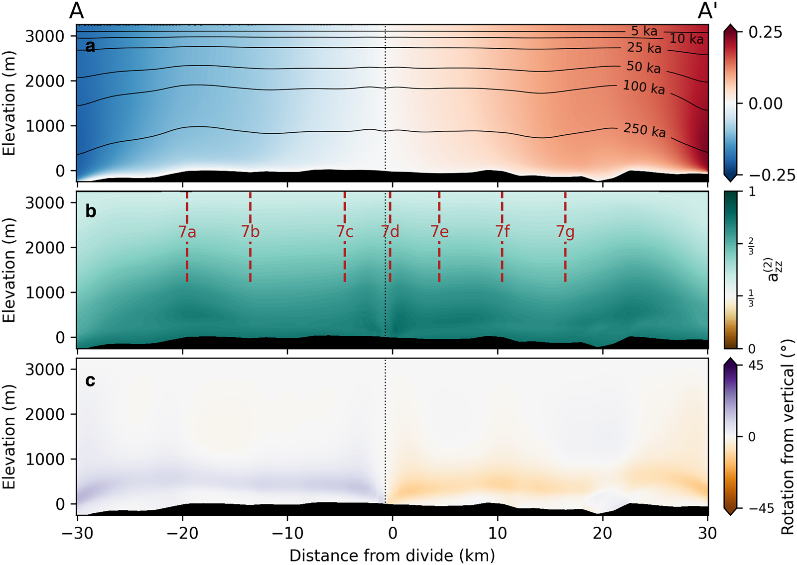
Figure 5. Model output along Dome C transect. (a) Horizontal speeds. Contours show ages of the ice. (b) Vertical component of the fabric. Vertical, red lines show locations of pRES acquisitions plotted in Figure 7; these data are a representative subset from Ershadi and others (Reference Ershadi2022). (c) Rotation of the fabric from vertical (degrees counter clockwise). In all panels, dotted black line shows the modeled, modern divide position.
The modeled horizontal ice-flow speed is very slow, reaching only 0.24 m a−1 at the edges of the model domain. These speeds agree well with GPS measurements of velocity in the area, which found speeds up to 0.21 m a−1 25 km from the divide (Vittuari and others, Reference Vittuari2004). However, those GPS measurements were not directly on the transect considered here, so more quantitative evaluation of the velocities is precluded.
The modeled ice divide was extremely stable in both position and thickness (Fig. 4). The ice thickness varied by ~10 m through the simulation, significantly <~250 m inferred from models that were specifically targeted at reconstructing surface elevations (Parrenin and others, Reference Parrenin2007b), while the divide position moved by only ~300 m (which is at the limit of the horizontal mesh resolution). The smaller variation in divide thickness is likely a result of the boundary conditions; regional ice thickness changes were not captured by the pseudo-pressure conditions used, but actual ice-thicknesses changes during the last 250 ka likely affected the entire continent. The lack of thickness change is thus a consequence of using a model domain with a finite width smaller than that of the continent; a model with no horizontal dimension can evolve freely as it is subject to only local conditions (e.g. Parrenin and others, Reference Parrenin2007b), and a continental-scale model can thicken or thin as a whole, but our limited domain depends on boundary conditions which do not permit such changes.
The modeled age profile shows a very minor double Raymond bump (maximum bump height 60 m, or 2% of the total thickness). Despite the extremely long characteristic timescale of the divide, the bump is allowed to form since model divide is so stable throughout the simulation. The double bump is characteristic of directional hardening due to fabric development (Martín and others, Reference Martín, Gudmundsson, Pritchard and Gagliardini2009), and has been observed over domes with shorter characteristic timescales (Goel and others, Reference Goel2020). Though there is not a Raymond bump in radar data in the area (Cavitte and others, Reference Cavitte2021), given the small amplitude of the modeled bump, and the overly stable modeled divide, this difference is unsurprising. Despite the relatively stable modeled divide, the bump amplitude is much smaller than the 10% of the ice thickness that would be expected in steady state (Goel and others, Reference Goel2020).
Model/data comparison
Ice-core measurements
We evaluate the modeled fabric at the modeled divide position, which is ~1 km southeast of the true position in all simulations (Fig. 6). Comparison at the closest approach to EDC yields similar results, but any effect of nonlinearity of the viscosity (i.e. the Raymond bump) is expected at the modeled rather than true divide, so the former provides the more fair comparison. At both the point of closest approach and at the modeled divide, the modeled fabric shows a weaker vertical component (λ 3) and one stronger horizontal component (λ 2) than was measured in the EDC core (Durand and others, Reference Durand2009). This difference is seen in the model both with laboratory and ice-core-calibrated rate factors, though it is significantly lessened for the ice-core-calibrated values. The model-data mismatch could be attributable to imperfect model physics describing the fabric development (due either to missing processes or poor parameterization), insufficiency of the simplified 2.5-D model to capture the stress state, temporal changes not considered by the model, or some combination of these (fabric regularization does not affect λ i much even for L = 6; see Appendix A). Diverging flowlines lead to a more dome-like stress state, and the flow direction is not well constrained right at the divide, so the assumptions of the 2.5-D model might break down in the center of the model domain (Passalacqua and others, Reference Passalacqua2016). Temporal changes in the large-scale flow could significantly alter our results; simulations extend back 250 ka, over which ice thickness is thought to have changed by >250 m (Parrenin and others, Reference Parrenin2007b), and accumulation patterns have likely changed even over the last 260 years, which suggests that migration of the divide is possible (Urbini and others, Reference Urbini2008). While we are able to incorporate local thickness and accumulation changes, such temporal changes are likely to have affected the large-scale flow of the ice sheet, and cannot be easily captured by a local model such as that used here. To further distinguish among possible causes of the model-data misfit, we compare our fabric results with pRES data along the model domain.

Figure 6. Comparison of modeled fabric (Elmer/Ice) and measured fabric from the EDC core (Durand and others, Reference Durand2009). Data are shown as squares. Colors indicate eigenvalue number (blue for λ 3, orange for λ 2 and green for λ 1). Model output is shown as lines, for both laboratory (solid) and ice-core (dashed) calibrated rate factors, with colors corresponding to the data.
Phase-sensitive radar
pRES returns are affected by ice-crystal fabric because the dielectric permittivity is different parallel and perpendicular to the c-axis of a single ice crystal (Fujita and others, Reference Fujita, Maeno and Matsuoka2006). In a typical radar geometry, returns are insensitive to the vertical component of the fabric but their strength and phase with azimuth is related to the horizontal anisotropy (e.g. Rathmann and others, Reference Rathmann2022). From these returns, it is thus possible, with minimal assumptions, to infer the difference in the horizontal eigenvalues of the fabric distribution (generally assumed to be the ODF). Recently published pRES measurements on a transect of Dome C (Corr and others, Reference Corr, Ritz and Martin2021; Ershadi and others, Reference Ershadi2022) therefore provide a way to test our modeled fabric field against observations, away from the ice-core site. Ershadi and others (Reference Ershadi2022) used these data to infer the difference between the horizontal eigenvalues and the orientation of the larger eigenvector with depth along the transect modeled here. Since our model does not capture rotation of the fabric out of the model plane, the modeled orientation of the largest eigenvalue is always transverse to flow; this agrees with all pRES measurements deeper than 500 m within error (shallower orientations are highly uncertain in the pRES due to weaker returns). We therefore compare only the difference in horizontal eigenvalues inferred from pRES and in the model output. We do so at seven of the sites (comparison at the remaining sites from Ershadi and others (Reference Ershadi2022) is shown as Supplementary Fig. S2).
Figure 7 shows the modeled and radar-inferred horizontal anisotropy at the seven sites marked in Figures 3 and 5. At the location of EDC, ice-core data are plotted as well (Durand and others, Reference Durand2009). Both the ice-core- and laboratory-calibrated models match the data well near the surface, but systematically find too-large horizontal anisotropy between 500 and 2000 m throughout the domain. Simulations with ice-core- and laboratory-calibrated recrystallization produce very similar horizontal anisotropy (negligible differences except deeper than 3000 m) despite large differences in the vertical component of the fabric. Differences compared to the pRES-inferred values reach a factor of 2.5 for both simulations. The pRES-inferred values match the EDC data well overall, although they generally lie at the low end of the spread in the ice-core data (Fig. 7d). The ice-core data thus suggest that some of the difference between the pRES-inferred anisotropy and the modeled anisotropy may be due to the pRES method slightly underestimating the eigenvalue difference. The majority of the model-pRES difference is therefore attributable to the model producing fabrics with too much horizontal anisotropy rather than errors in the pRES measurements.
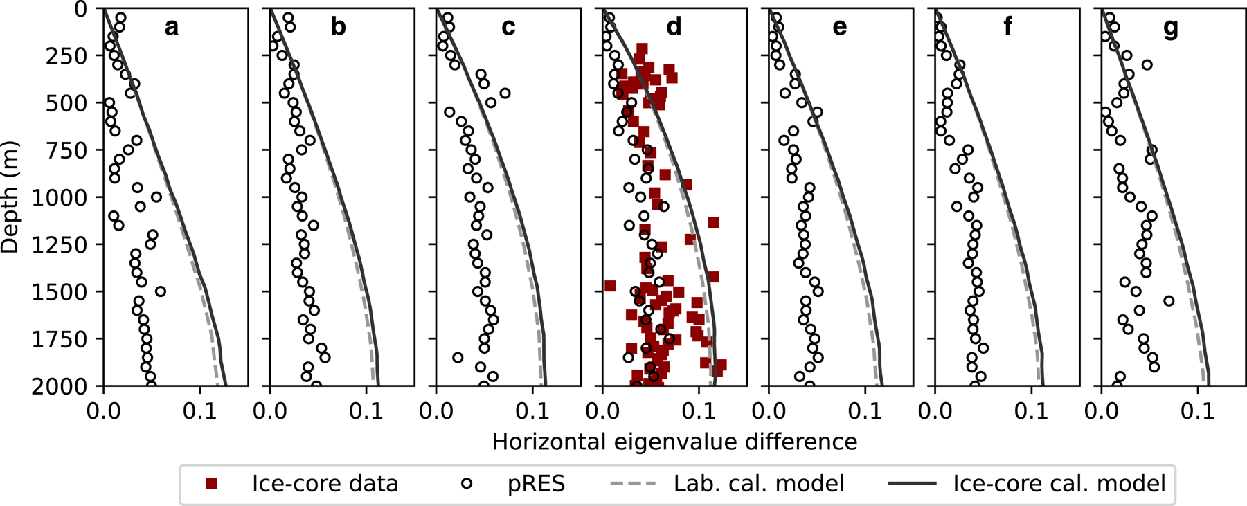
Figure 7. Horizontal eigenvalue difference of modeled and pRES-inferred fabric (Ershadi and others, Reference Ershadi2022) at locations shown in Figures 3 and 5. (a–g) are E18, E12, E3, EPICA, W6, W12 and W18 from Ershadi and others (Reference Ershadi2022). pRES is shown with black circles, ice-core-calibrated model with dark gray lines, laboratory-calibrated model with dashed, light gray lines and the EDC core with red (only where the pRES and model coincide with the core). Remaining sites from Ershadi and others (Reference Ershadi2022) are shown in Supplementary Figure S2.
Discussion
Implications of model-data misfit
Using ice-core- or laboratory-calibrated rate factors, the model produces slightly too strong horizontal anisotropy throughout the model domain. Given this difference and the available data from EDC, it is reasonable to infer that the vertical component of the modeled fabric is too weak throughout the domain as well. Although we are unable to attribute the model-data misfit to a single cause, it seems likely that the differences are, in large part, due to limitations of the fabric model rather than of the ice-flow model, time-dependent forcing or boundary conditions. Since the fabric model considers the processes thought to be most relevant for fabric development, and the model can qualitatively reproduce fabrics found in ice cores and laboratory deformation experiments, we consider assumptions about the rates of these processes to be the most likely cause of the model-data misfit.
Although the rate-factor parameterizations (Γ0 and Λ0) of the different fabric processes are only approximations of the true physics of fabric development, they are qualitatively able to produce the diversity of natural and synthetic fabrics (Richards and others, Reference Richards, Pegler, Piazolo and Harlen2021). We consider it likely that the rate factors are not accurately described by either set of coefficients (lab- or ice-core-calibrated coefficients), and that further calibration against experimental data could yield a closer match to the data, without large changes to the models of fabric processes (i.e. the functional form of Eqn (5)). Indeed, laboratory-calibrated rates were effectively tuned to three data points without uncertainty bounds (Richards and others, Reference Richards, Pegler, Piazolo and Harlen2021). Additional laboratory measurements, designed to allow the rate factors to be tuned against data (at different strain rates, temperatures and stresses), might lead to better constrained coefficient functions of the recrystallization models, and might clarify whether the model-data mismatch is due to sparse experimental data.
Similarly, calibrating the coefficient functions by comparing data from EDC to a one-dimensional, time-varying model with a better-constrained strain tensor, might change the ice-core-calibrated values and elucidate whether the model is capable of exactly reproducing the data. For example, it is possible that further data will clarify whether the rate of migration recrystallization is truly linear in the strain rate or whether a more complicated relationship exists; given the difference in strain rates in the laboratory and natural settings, a rate factor that depends non-linearly on the strain rate may reconcile our estimated coefficients.
Calibration to ice cores drilled in more complex flow regimes could provide additional information about this difference. Fabric measurements on the EastGRIP core (Westhoff and others, Reference Westhoff2021) could be particularly valuable for calibration, since it samples an active ice stream moving 50 m a−1. Measurements on NEEM (Montagnat and others, Reference Montagnat2014), drilled on a divide rather than a dome, and the South Pole ice core (Voigt, Reference Voigt2017), drilled on a flank moving 10 m a−1 would add two more stress states for calibration. Multi-site calibration requires a more efficient approach than the brute-force method used here, and the more complex stress states may not be accurately simulated with the simple Nye and Dansgaard–Johnsen models used here. Nevertheless, such multi-site calibration may help elucidate whether site-specific characteristics of Dome C, for example the cold temperature and low strain rates, explain some of the difference between our ice-core- and laboratory-calibrated rate factors.
Large-scale modeling with a spectral fabric description
There are important differences between the spectral and tensorial representations both in terms of physics and in terms of technical implementation (Richards and others, Reference Richards, Pegler, Piazolo and Harlen2021; Rathmann and others, Reference Rathmann, Hvidberg, Grinsted, Lilien and Dahl-Jensen2021). A clear advantage of the spectral formulation is that it does not need a closure approximation, while consistency requires at least a minimal closure for a tensorial representation. Definitionally, each high-order structure tensor must have a number of non-zero components leading to the sub-traces taking values compatible with the lower-order structure tensors (e.g. Advani and Tucker, Reference Advani and Tucker1987). This becomes problematic when the evolution of lower-order tensors depends on the higher-order ones, since the higher-order contributions cannot ever be assumed to be zero. In the spectral representation, harmonics with l > 0 represent anomalies relative to isotropy, modes >L can safely be ignored for fabric development (an equivalent assumption can be made for the tensorial representation, but since for isotropic fabrics the higher-order tensors are non-zero it is more complicated than assuming spectral components are zero).
Perhaps the most important physical disadvantage to the spectral approach is the need to balance regularization (in orientation space) with the maximum fabric strength that is possible. For example, using canonical Laplacian regularization with L = 6, λ 3 saturates ~0.8 in unconfined compression, while λ 3 → 1 is expected under sufficient strain; we avoided this problem with carefully calibrated hyper diffusion that permitted λ 3 > 0.99 while keeping the model stable. Such calibration must, however, be adjusted for different values of L, or else spurious oscillations or a maximum fabric strength will result.
In addition to physical differences, there are a number of technical differences between the spectral and tensorial representations that affect the feasibility of using the two representations in a large-scale model. We briefly mention the two that we see as most important. At the same order of truncation, the spectral and tensorial representations have the same number of degrees of freedom. With no simplifications, the spectral representation always tracks two times the number of complex, independent components (plus the zero-order component), while the tensorial representation, in native form, tracks a number of degenerate components that increases proportional to 3m. For example, a(4) has 81 components, but only nine are unique (assuming a(2) is known); in order to avoid the computational cost of tracking all 81, however, cumbersome expressions must be derived for each individual independent component. This rapidly becomes infeasible if yet higher-order structures are desired. Even if only a(2) and a(4) were explicitly tracked, modeling the evolution of a(4) would require an approximation of the non-zero elements of a(6), which has only 15 independent components out of its 729 elements. The tedious work of determining these relations is avoided with the spectral representation; the simplifications of Eqn (13) remain the same at each L, and can be handled automatically to reduce the problem to only the independent components. Thus, the lack of degeneracy allows us to increase the order of the fabric description up to any desired order, so future studies with greater computational power and some need for highly resolved representations of the fabric could use arbitrarily large L (we tested up to L = 12, but expect larger L to be feasible with greater computational resources).
Another technical difference is that some models of fabric process (e.g. DDRX) naturally involve a(m), whereas others (e.g. lattice rotation and CDRX) involve ϱ*, which might influence the choice of representation. Apart from having to construct structure tensors when comparing modeled fabrics to ice-core measurements, constructing a(2) and a(4) – even when DDRX is negligible – is necessary in the spectral approach since the eigenenhancements, E ij, (or fluidity tensor) depend on both a(2) and a(4). Reconstructing a(2) and a(4) is quick compared to the time taken to model the evolution of ϱ*(x, t) in 2-D, so does not add significant computational cost. Relatedly, all a(m) lie between 0 and 1 by definition, but may fall outside this range due to numerical or truncation errors. Enforcing these bounds by renormalizing a(m) (e.g. dividing through by the sum of unnormalized eigenvalues and setting negative eigenvalues to zero) becomes increasingly tedious for structure tensors of increasing order m > 4, as determining eigenvalues becomes increasingly computationally difficult. In the spectral approach, we found it useful to cap the angular power spectrum of $\hat \varrho _l^m$ to ensure the largest eigenvalue is ≤1 for all a(m); to do so, we renormalize the power spectrum to that of the delta function if needed (representing a perfect single maximum). Because of the way the harmonic modes describe an anomaly from isotropy, this in turn also ensures the smallest eigenvalue is ≥0. While this does not ensure the smallest eigenvalues are ≥0 for relatively strong girdle fabrics, such fabrics do not arise in the present simulations. If renormalization is not carefully addressed, this can lead to numerical issues – particularly for strong single-maximum fabrics – caused by spectral coefficients resulting in negative directional viscosities (see Appendix A).
Outlook
The spectral representation of fabric provides a convenient way to include additional processes in modeling of fabric evolution, and thus provides a path forward for integrating future small-scale model development into large-scale ice-flow models. Simply moving to L > 2 permitted us to model the effect of DDRX, and further increases in the order of approximation could allow for use of nonlinear grain rheologies in deriving the bulk anisotropic fluidity; such a transition is greatly eased by the spectral representation of the fabric. The contrast between fabric modeled with laboratory- and ice-core-calibrated rate factors suggests a disconnect between how fabric develops in the laboratory and in natural settings; presumably this difference stems from the 5–7 orders of magnitude larger strain rates at which laboratory tests are conducted compared to typical ice-core settings. Some fundamental differences have been clear before this work; for example, laboratory ice-deformation experiments do not seem to produce strong girdles, despite widespread observations of girdles in natural ice. This modeling, and the recent work on which it relies (Richards and others, Reference Richards, Pegler, Piazolo and Harlen2021; Rathmann and Lilien, Reference Rathmann and Lilien2022b), allows direct comparison of the fabric evolution at laboratory scales/rates and ice-core scales/rates, potentially providing a path forward for understanding these differences.
In this work we have avoided areas with rapid ice flow, since data with which to validate the model are unavailable in such areas. However, accurately capturing rheology in areas of fast flow is critical for accurate modeling of outlet glaciers and ice streams. For example, models that do not include anisotropy sometimes find that ad-hoc weakening of shear margins (beyond the weakening expected from temperature alone) produces a better match to velocity observations (e.g. Joughin and others, Reference Joughin2012). Such weakening is often attributed to anisotropy (Minchew and others, Reference Minchew, Meyer, Robel, Gudmundsson and Simons2018; Grinsted and others, Reference Grinsted2022). The complexity of flow in such areas necessitates a relatively complex fabric model such as that used here. Shear margins have relatively short residence times, so fabric cannot be assumed to be in steady state with its in situ stress state, precluding the use of models that make such an assumption (Graham and others, Reference Graham, Morlighem, Warner and Treverrow2018), yet recrystallization is thought to be active at the relatively high temperatures and high strain rates found in shear margins (Faria and others, Reference Faria, Weikusat and Azuma2014; Hunter and others, Reference Hunter, Meyer, Minchew, Haseloff and Rempel2021), precluding a(2)-only approaches. Moreover, the multiple deformation modes active in shear margins (transition from vertical shear to plug flow coincident with horizontal shear) suggest a need to use a tensorially anisotropic viscosity. Fabric will evolve through time, and will do so differently from other potential modes of weakening, such as crevassing, so the need to capture the full fabric field and its evolution is compounded in transient simulations. The model presented here could be applied to areas with multiple active deformation modes, such as shear margins, to more accurately capture the variations in directional viscosity and the evolution of flow through time, an application for which existing anisotropic models are not calibrated. Further calibration of this model to use in such areas could take advantage of additional geophysical constraints, such as seismics (e.g. Lutz and others, Reference Lutz2022), in order to validate modeled fabric in these areas.
Conclusions
We incorporated a recently developed model of fabric evolution into a large-scale ice-flow model. The model includes lattice rotation, rotation recrystallization and migration recrystallization, the three processes thought to be most important for fabric development, and couples the fabric to ice flow through a rheology with fewer approximations than those used previously. We applied this new, coupled model to simulate ice flow and fabric development on a transect across Dome C, East Antarctica, where relatively plentiful validation data exist. At the small scale, previous work showed that this model does an excellent job reproducing laboratory fabric-development experiments (Richards and others, Reference Richards, Pegler, Piazolo and Harlen2021), but applying it to the large scale, as we have done here, reveals that the model is less able to reproduce the large-scale fabric found in the EDC core and inferred from pRES. Calibrating rate factors to match the EDC core, using a zero-dimensional model, reduced, but did not eliminate, this misfit. This discrepancy cannot be firmly attributed to one source, but insufficient constraints on the relative rates of different processes (migration recrystallization, rotation recrystallization and lattice rotation) may be the cause. The difference found between calibrated process rate factors using laboratory and ice-core data suggests a gap exists in our understanding of how ice-crystal fabric develops differently in laboratory compared to natural (in situ) conditions. However, this type of modeling allows quantitative comparison across spatial and temporal scales, and thus provides a potential path forward for reconciling the differences of fabric development found in laboratory and natural conditions. The model is one of the first that is well-suited to simulating the effect of fabric on the complex deformation experienced in areas such as shear margins, and may thus allow more accurate simulation of such areas.
Supplementary material
The supplementary material for this article can be found at https://doi.org/10.1017/jog.2023.78.
Data
All data used in this study are available as part of previously published work. The version of Elmer/Ice, with new solvers, can be found at https://doi.org/10.5281/zenodo.7415785. The version of SpecFab used here can be found at https://doi.org/10.5281/zenodo.7416060. Code to run all simulations and produce all figures can is archived at https://doi.org/10.5281/zenodo.8200402.
Acknowledgements
David Lilien, Nicholas Rathmann, Christine Hvidberg, Aslak Grinsted and Dorthe Dahl-Jensen were supported by the Villum Foundation through the IceFlow project (No. 16572). David Lilien and Dorthe Dahl-Jensen were further supported by funding from the Canada Excellence Research Chairs Program. Reza Ershadi and Reinhard Drews were supported by German Research Foundation (DFG) Emmy Noether grant No. DR 822/3-1. The authors thank editors Ralph Greve and Sergio Faria and two anonymous reviewers for valuable comments that improved the clarity of the manuscript and robustness of the results.
Author contributions
David Lilien coupled the fabric model to Elmer/Ice, performed the simulations, and wrote most of the paper. Nicholas Rathmann developed the spectral model and designed model validation experiments. Christine Hvidberg, Aslak Grinsted and Dorthe Dahl-Jensen provided guidance and feedback on model development, validation and simulations. Dorthe Dahl-Jensen also secured funding. Reinhard Drews and Reza Ershadi provided inverse results from pRES and helped interpret the model/radar comparison. All authors contributed to editing the final manuscript.
Appendix A: Fabric evolution model validation
We performed a number of ‘cube crushing’ experiments to test the performance of the spectral fabric description in Elmer/Ice. Simulations are split into two- and three-dimensions; when the velocity gradient in one direction is uniformly zero (e.g. ∂u/∂z = 0) it is sufficient to use a 2-D model, but when there are non-zero velocity gradients in all three directions a 3-D model is required. Model domains were 1 m cubes in 3-D (1 m squares in 2-D) with 5 cm mesh resolution. Four types of strain were applied: simple shear (in x–y), confined compression (compression in y, confined in z), unconfined compression (in z) and uniform extension (in z). The former two used 2-D domains and the latter two used 3-D. All used a strain rate of 0.1 a−1, which was uniform across the whole model domain (i.e. the velocity was fixed rather than simulated). For each strain, seven simulations were run:
(1) Full fabric model (Γ0 = 0.55 a−1 and Λ0 = 2.0 × 10⁻² a−1, chosen to approximate rates at $-5^\circ$
 C).
C).(2) Lattice rotation only (Γ0 = 0 a−1 and Λ0 = 7 × 10⁻³ a−1 for regularization).
(3) Migration recrystallization only (Γ0 = 0.55 a−1 and Λ0 = 0 a−1, no lattice rotation).
(4) Full fabric model (Γ0 = 0.55 a−1 and Λ0 = 2.0 × 10⁻² a−1), but replacing the stress with the strain rate in Eqn (10) for comparison with prior work.
(5) Migration recrystallization only (Γ0 = 0.55 a−1 and Λ0 = 0 a−1, no lattice rotation), but replacing the stress with the strain rate in Eqn (10) for comparison with prior work.
(6) Full fabric model (Γ0 = 0.73 a−1 and Λ0 = 2.0 × 10⁻² a−1, chosen to approximate rates at $0^\circ$
C).(7) Full fabric model (Γ0 = 0.17 a−1 and Λ0 = 1.7 × 10⁻² a−1, chosen to approximate rates at $-30^\circ$
C).


Pure-shear simulations (extension and compression) were run to 100% strain using ~0.09 year time steps, while the simple shear simulations were run to 300% strain using 0.06 year time steps. During the simulations, the mesh was fixed; this leads to inflow boundaries where we assume that isotropic ice enters. Results are considered at the center point of the cube or square, where u = 0 and thus there are no advective effects.
The cube-crushing experiments were matched to simulations using the tensorial fabric representation in Elmer/Ice (which necessarily considered only lattice rotation) and simulations of a single, zero-dimensional ice parcel using SpecFab. Methods for the tensorial representation followed previous work exactly (Gillet-Chaulet and others, Reference Gillet-Chaulet, Gagliardini, Meyssonnier, Zwinger and Ruokolainen2006; Lilien and others, Reference Lilien, Rathmann, Hvidberg and Dahl-Jensen2021), so model equations are not repeated here. These simulations allow us to isolate the effect of using the higher-order fabric model, where closure assumptions do not affect the lower order fabric moments, on lattice rotation. Three SpecFab simulations were run for each strain-rate experiment: one with the full fabric model using parameters for $-5^\circ$ C, one with lattice rotation only (and rotation recrystallization for regularization) and one with migration recrystallization only. For migration recrystallization in SpecFab, the strain rate was used to determine D in Eqn (10) (i.e. the stress and strain rate were assumed to be coaxial). SpecFab simulations used L = 20, which allows us to identify the limitations of truncating the fabric description at L = 6. In the full and lattice rotation simulations, we used hyper diffusion for regularization, with identical coefficients to those used with Elmer/Ice.
Lattice rotation
Results from the cube-crushing experiments are shown in Figure 8. The model output closely matches laboratory data for unconfined compression (Hunter and others, Reference Hunter, Meyer, Minchew, Haseloff and Rempel2021), while it matches less well for simple shear (Qi and others, Reference Qi2019); however, the laboratory measurements are run to a lower total strain than used here, which may partially explain this difference. Using the higher-order, spectral representation of fabric leads to significant differences compared with the tensorial representation in the case of simple shear (middle column of panel b in Fig. 8). There was a near-perfect match between the spectral and tensorial representations for pure shear simulations (middle column of panels a, c and d in Fig. 8). Example fabrics produced by lattice rotation alone can be seen in Figures 9a, f. For lattice rotation, the SpecFab version should be thought of as ‘truth’ in the sense that differences between the other models and the SpecFab version are solely due to the lower-order representation of the fabric and regularization (for the spectral version). The spectral implementation in Elmer, despite being lower order and including spatial regularization, exactly matches the SpecFab version except for confined compression. In that case, the very strong single maximum that forms is limited in strength by the spatial resolution and regularization; because the fabric gradient here is much stronger than in larger-scale models (isotropy to a single maximum in 0.5 m), this limitation will not affect realistic, large-scale applications. The tensorial representation produces results remarkably close to the SpecFab ‘true’ version except in the case of simple shear; this difference likely stems from the tuning of the closure approximation in the tensorial approach. This mismatch implies that even when lattice rotation alone is considered, a higher-order model may be justified for areas experiencing simple shear.

Figure 8. Results from cube crushing simulations at $-5^\circ$ C, showing eigenvalues of the simulated fabric under (a) confined compression, (b) simple shear, (c) unconfined compression and (d) uniform extension. Within each panel, the three columns indicate which processes are included. Solid lines show laboratory deformation test results simple shear run to 260% strain at −5$^\circ$
 C) (PIL94; Qi and others, Reference Qi2019), and unconfined compression to 40% strain at $-3^\circ$
 C at two different strain rates (MD22 and D5-1; Hunter and others, Reference Hunter, Wilson and Luzin2023). Dashed lines show eigenvalues under lattice rotation only using the structure-tensor representation of fabric in Elmer. Markers show other simulation types (SpecFab, Elmer spectral with DDRX calculated using τ, or Elmer spectral with DDRX calculated using ${\dot {\boldsymbol \epsilon }}$
 ). Colors indicate eigenvalue number (blue for λ 3, orange for λ 2 and green for λ 1).

Figure 9. Temperature dependence of modeled fabric. (a–e) Fabric under simple shear in x–y with lattice rotation only, at $-30^\circ$ C, at $-5^\circ$
 C at $0^\circ$
 C, and with DDRX only respectively; since recrystallization increases with temperature, pure lattice rotation or DDRX can be seen as end members of a spectrum (although neither is ever achieved). (f–j) as in (a–e), but for uniform extension in z. (k–n) Dependence of the fabric eigenvalues on temperature under different strains. Colors indicate eigenvalue number (blue for λ 3, orange for λ 2 and green for λ 1). Lines with squares indicate model results. Diamonds, X's and circles show laboratory data from PIL007, PIL94, PIL135 and PIL268 of Qi and others (Reference Qi2019), PIL255 Fan and others (Reference Fan2020) and MD22, D5-3 and D5-1 of Hunter and others (Reference Hunter, Wilson and Luzin2023), respectively; symbols with white centers indicate that the total strain used in the laboratory experiment is significantly less than that used in the simulation (<40% compared to 100% used in the model).
Migration recrystallization
When only migration recrystallization is active, the model produces the multi-maxima and 45$^\circ$ pseudo-girdle fabrics that are considered indicative of migration recrystallization (Figs 9e, j). For the cases tested, we find very little sensitivity to whether τ or ${\dot {\boldsymbol \epsilon }}$
 is used to determine the migration recrystallization in Eqn (10). This is not a guarantee that using ${\dot {\boldsymbol \epsilon }}$
 is always appropriate, though. As seen in the ‘full’ column of each panel of Figure 8, interplay lattice rotation and recrystallization can cause subtle differences to emerge based on whether the migration recrystallization is τ- or ${\dot {\boldsymbol \epsilon }}$
 -dependent.
Full fabric model
The full fabric evolution, including both migration recrystallization and lattice rotation, is intermediate between the lattice-rotation-only and migration-recrystallization-only fabrics (Fig. 8). However, the complex, multi-maxima or 45$^\circ$ pseudo-girdle are not seen in the coupled simulations. Nevertheless, the differences compared with the lattice-rotation only simulations are significant (up to 50% difference in eigenvalues, Figs 9k–n), so recrystallization still has an important effect. However, differences are only notable at high temperatures (Fig. 9). Nonetheless, the effects of recrystallization suggest that its effects should be considered even at lower temperatures, consistent with prior work (Richards and others, Reference Richards, Pegler, Piazolo and Harlen2021).
Effect of truncation and regularization
Unless regularization is added to the dynamical model of fabric evolution (5), a quasi-periodic trajectory is found in the state space of the expansion coefficients, $\hat \varrho _l^m$ , that may pass through unphysical states where the resulting eigenvalues of a(m) fall outside their normalized bounds (between 0 and 1). As noted in the main text, we apply hyper-diffusion with a magnitude sufficiently large as to guarantee stable states are approached under sustained, constant modes of deformation with lattice rotation. Laplacian diffusion is a spectrally broad operator that affects several modes near l = L. When L = 6, this has the consequence of preventing the coefficients $\hat \varrho _2^m$
 and $\hat \varrho _4^m$
 from taking the values needed to represent concentrated c-axis distributions, such as a strong single maximum. Like in classical fluid problems posed in spectral space, diffusion can be spectrally sharpened to affect a minimal number of high-wavenumber modes (high l). Figure 10 shows the difference between applying an unmodified Laplacian operator as regularization (light lines) as opposed to hyper diffusion (dark lines). For the same truncation order L, it is clear that unless hyper diffusion is considered, the largest a(2) eigenvalue (upper x-axis in Fig. 10) is limited to take values of λ 3 ≤ ~0.8, which limits the corresponding largest and smallest directional enhancement factors (E ij) that can be modeled (filled and line contours). Similarly, if a higher-order truncation (L = 20) is considered, Figure 10 shows that the effect of regularization (unmodified or hyper diffusion) is not felt at the lowest wavenumber coefficients, $\hat \varrho _2^m$
 and $\hat \varrho _4^m$
 . While large L are therefore to be preferred (guaranteeing that the dynamics of the coarsest-scale structure in the MODFs is governed by lattice rotation and DDRX, and not regularization), computational resources in practice limit how large L can be taken to be; in our case, the very long simulation prevented us from considering L > 6. Hyper diffusion was thus necessary for such a simulation.

Figure 10. Modeled fabric state trajectories (lines) and the corresponding eigenenhancements (filled and line contours) for vertically symmetric fabrics similar to Figure 1. Modeled fabric trajectories are shown for regularization with (dark lines) and without (light lines) hyper diffusion. Hatched area indicates restricted parts of the state space, bounded by the angular power spectrum not being allowed to exceed that of the delta function (perfect single maximum); see main text.
Appendix B: Orthotropic rheology validation
We compare the effect of using the full nonlinear orthotropic viscosity of Rathmann and Lilien (Reference Rathmann and Lilien2022b) for using the nonlinear extension to the general orthotropic linear flow law (GOLF; Gillet-Chaulet and others, Reference Gillet-Chaulet, Gagliardini, Meyssonnier, Montagnat and Castelnau2005) that, by analogy to the canonical Glen's flow law, introduces a nonlinear viscosity depending solely on the second invariant of the deviatoric stress tensor (Martín and others, Reference Martín, Gudmundsson, Pritchard and Gagliardini2009). In the GOLF,

where $\tilde {\eta }_0 = A^{-1/n}( \epsilon_{{\rm E}}^{(1-n)/2n})/4$ is an isotropic effective viscosity related to the canonical Glen prefactor, $\tilde {\eta }_{i} = \tilde {\eta }_{i} ( {\bf a}^{( 2) })$
 are six dimensionless viscosities (that differ from Eqn (20)), and dev( ⋅ ) denotes the deviatoric part of a tensor. The viscosities $\tilde {\eta }_{i}( {\boldsymbol a}^{( 2) })$
 were taken from the visco-plastic self-consistent model of Gillet-Chaulet and others (Reference Gillet-Chaulet, Gagliardini, Meyssonnier, Zwinger and Ruokolainen2006). Note that for an isotropic fabric, this relation reduces to the ordinary form of Glen's flow law, just as for the full nonlinear orthotropic version.
There are two essential differences between the full nonlinear orthotropic law used here and the GOLF: (1) the nonlinear viscosity differs as a result of which invariants are considered and (2) the directional enhancement factors differ as a result of different homogenization schemes (linear combination of Taylor and Sachs hypotheses for the full nonlinear orthotropic law, visco-plastic self-consistent model (VPSC) for the GOLF). Rathmann and Lilien (Reference Rathmann and Lilien2022b) showed that the approximated rheology generally does a good job reproducing the unapproximated form to a small relative error for a given fabric, but did not consider the accumulation of such errors as a coupled simulation progressed.
To assess whether the full nonlinear rheology was likely to be important in more realistic settings (and thus in parts of the Dome C transect), we ran three simulations of an idealized ice divide, similar to those in Martín and others (Reference Martín, Gudmundsson, Pritchard and Gagliardini2009) but using the spectral formulation for the fabric, and including recrystallization and an evolving temperature field. We used the ice-core-calibrated rates for recrystallization, since this generally produces stronger fabrics and thus may show a larger difference between the rheologies. The three simulations differed only in the rheology: one used the canonical Glen's flow law, one used the nonlinear extension to the GOLF and the third used the full nonlinear orthotropic rheology. The model domain was 40 km wide, ice was 2 km thick at the outflows (with the divide in the center) and mesh resolution was 75 m in the vertical and 300 m in the horizontal. The outflows used the same pseudo-glaciostatic boundary condition as the Dome C simulations, with d′ = 2000 m, and there was no sliding. The ice surface was held at $-40^\circ$ C, and there was 75 mW m−2 of geothermal heat. Accumulation was 0.05 m a−1 (making the timescale $\tau = H/\dot {b} = 40$
 ka). The simulations started with isotropic fabric and ran for 5τ = 200 ka, which is not long enough to reach steady state but is long enough to show anisotropic effects (Martín and others, Reference Martín, Gudmundsson, Pritchard and Gagliardini2009). The full nonlinear rheology produces a result intermediate between Glen's law and the GOLF (Fig. 11). Differences compared to the GOLF are most pronounced near the divide. Because the nonlinear extension to the GOLF closely matches the full nonlinear orthotropic law (Rathmann and Lilien, Reference Rathmann and Lilien2022b), these differences are likely due to feedbacks between fabric development and flow that lead to the small differences slowly accumulating to larger departures. An additional aspect of the difference may be due to the differences between the VPSC and the linear combination of the Taylor and Sachs hypotheses; the present work cannot identify the effect of that difference. We note that the results here differ significantly from Martín and others (Reference Martín, Gudmundsson, Pritchard and Gagliardini2009), which found a double Raymond bump and a stronger difference between their anisotropic rheology and Glen's flow law. Most of this difference can be attributed to recrystallization; in our model migration recrystallization introduces other fabric patterns, and rotation recrystallization causes decay toward isotropy. Both of these prevent the effects of anisotropy from being as strong under the divide, which combines with the limits that L = 6 places how hard the ice can become for (vertical) compression (see Appendix A). In addition, the cold temperatures and low accumulation in our model contrast with Martín and others (Reference Martín, Gudmundsson, Pritchard and Gagliardini2009), who were mainly interested in ice rises. Our comparison is relevant for the area at hand, but other areas with shorter timescales, or where recrystallization is not thought to be active, may show much larger differences between rheologies.

Figure 11. Effect of different rheologies on an idealized ice divide. (a) Age structure of the divide. Blue, red and brown contours show isochrones at various ages for Glen's flow law, the unapproximated nonlinear orthotropic rheology and the nonlinear extension to the GOLF (Martín and others, Reference Martín, Gudmundsson, Pritchard and Gagliardini2009), respectively. Contours for Glen's law are mostly covered by those for the unapproximated nonlinear orthotropic rheology. (b) As in (a), but with contours of $\vert \dot {\epsilon }_{xz}\vert$ .
.


 Open access