


1. Introduction
Melt from mountain glaciers accounted for nearly one third of global sea level rise over the period 2000–19 due to their strongly negative mass balance, despite representing only 1% of global glacier ice volume (Hugonnet and others, Reference Hugonnet2021). In the Alaska-Yukon region, glaciers experienced a total mass loss of approximately 3000 Gt, or 8 mm sea-level equivalent (s.l.e.), from 1961 to 2016 (Zemp and others, Reference Zemp2019). Alaska-Yukon is currently equal with the Canadian Arctic for the region with the largest total glacier mass loss globally, with an average rate of 73 ± 17 Gt a−1 from 2002–19 from both satellite gravimetry observations and geodetic mass balance measurements (Zemp and others, Reference Zemp2019; Ciracì and others, Reference Ciracì, Velicogna and Swenson2020). Ciracì and others (Reference Ciracì, Velicogna and Swenson2020) also measured an acceleration in mass loss of 2.8 ± 0.5 Gt a−2 for Alaska-Yukon over the period 2002–19.
The glaciers of the St. Elias Mountains in Alaska-Yukon cover an area of ~ 25 000 km2. Past studies have determined their thinning rate to average ~0.78 ± 0.34 m a−1 w.e. over the period 1958 to 2008, with increasing losses in low elevation regions, and negligible thinning in the accumulation area at higher elevations (Barrand and Sharp, Reference Barrand and Sharp2010; Foy and others, Reference Foy, Copland, Zdanowicz, Demuth and Hopkinson2011; Kienholz and others, Reference Kienholz2015; Larsen and others, Reference Larsen2015; Young and others, Reference Young, Flowers, Berthier and Latto2020). In addition, this region will continue to contribute significantly to sea-level rise beyond the current century, as the large volume of ice will ensure that glaciers persist, unlike other regions, such as Central Europe and the Caucasus, which are expected to lose most of their glacier cover by the second half of this century (Zemp and others, Reference Zemp2019).
The St. Elias region has experienced an accelerated, elevation-dependent warming since 1979, with elevations between 5500 and 6000 m above sea level (asl) warming at a rate ~1.6 times greater than the global average over the period 1970–2015 (Williamson and others, Reference Williamson2020). Furthermore, mean annual air temperatures are expected to increase by an additional 3.0 to 3.5°C for the region by 2099 (Solomon and others, Reference Solomon2007). With all these factors considered, there is a significant committed ice loss from this region, as glacier losses are not in balance with the present climate (Zemp and others, Reference Zemp2019; Young and others, Reference Young, Flowers, Berthier and Latto2020). For example, Young and others (Reference Young, Flowers, Berthier and Latto2020) estimate a committed terminus retreat of ~23 km and ice loss of 46 km3 for Kaskawulsh Glacier based on the 2007–18 climate.
As Kaskawulsh Glacier (Fig. 1) has lost mass, terminus retreat has opened space for two proglacial lakes to form and grow, particularly since the start of the 21st century. However, in May 2016 the largest of these, Slims Lake (Fig. 1), drained rapidly through an ice-walled channel, lowering the lake level by 17 m (Shugar and others, Reference Shugar2017). This re-routed meltwater away from Ä’äy Chù (Slims River), through the new channel and into the Kaskawulsh River and then Alsek River, with significant impacts to the regional drainage system, including changes in sediment transport, fish populations and ice conditions for local communities (Bachelder and others, Reference Bachelder2020). Studies elsewhere suggest that the presence of a large glacial lake can initiate terminus floatation, which even at a localised level, can reduce basal friction and increase velocities (Benn and others, Reference Benn, Warren and Mottram2007). Nothing is known of how these proglacial lake changes have impacted the dynamics of Kaskawulsh Glacier, but considering that proglacial lake volume has increased recently in the Alaska-Yukon region and is likely to continue to increase globally, this information is important to inform ice flow models, sea level rise predictions, and how glaciers will respond to a warming climate (Field and others, Reference Field, Armstrong and Huss2021).

Fig. 1. Kaskawulsh Glacier terminus region showing main locations referred to in the text. Base image: Sentinel-2, 3 August 2019, UTM Zone 7N. Inset: Regional map of Kluane National Park within the St Elias Mountains (red outline), with location of Kaskawulsh Glacier highlighted; source: Yukon Geological Survey, with glacier outlines from RGI v. 6.0 (RGI Consortium 2017). MLP, Mountain Legacy Project. Transects G-G′, H-H′, and I-I′ are identical to those in Waechter and others, Reference Waechter, Copland and Herdes2015.
This paper undertakes the first century-scale analysis of changes of the terminus (lowermost 10 km) of Kaskawulsh Glacier, one of the largest outlet glaciers in the St. Elias Mountains, containing ~9% of total glacier ice volume in the Yukon (Farinotti and others, Reference Farinotti2019). We build on previous studies to extend the terminus position record back to the late 1800's, undertake an analysis of long-term changes in ice thickness, and examine how surface velocities have evolved through the growth and drainage of proglacial lakes at the terminus since the 1980s.
2. Study area
Kaskawulsh Glacier (60°45′00″N, 139°08′37″W), or Tänshį in the Southern Tutchone language, is located on the eastern flank of the St. Elias Mountains in the Donjek Range, Yukon (Fig. 1). Covering an area of 1096 km2, this valley glacier measures ~70 km in length and is up to 6 km wide (Young and others, Reference Young, Flowers, Berthier and Latto2020). Kaskawulsh Glacier is divided into three main arms. The North and Central Arms are supplied by the Kluane Icefields, with an accumulation area bordering Sít' Tlein (Hubbard Glacier) at ~2500 m asl, while the South Arm is sustained by a separate, more southerly catchment (Foy and others, Reference Foy, Copland, Zdanowicz, Demuth and Hopkinson2011; Flowers and others, Reference Flowers, Copland and Schoof2014). The glacier terminates at ~760 m asl, and radiocarbon dating of trees exposed at the terminus, along with the time required for Picea glauca (white spruce) to re-establish after ice retreat (Denton and Stuiver, Reference Denton, Stuiver, Bushnell and Ragle1967), suggests that the Little Ice Age maximum extent was reached between the early- to mid-1700s (Reyes and others, Reference Reyes, Luckman, Smith, Clague and Van Dorp2006) and 1836 (Borns and Goldthwait, Reference Borns and Goldthwait1966).
Kaskawulsh Glacier is one of only a few large glaciers on the eastern flank of the St. Elias Mountains not known to surge (Young and others, Reference Young, Flowers, Berthier and Latto2020), with Waechter and others (Reference Waechter, Copland and Herdes2015) showing that it had undergone few significant changes in velocity over most of its length from 1960–2012 except for a slowdown in the lowermost ablation area, ~10 km from the terminus. The glacier thinned at an average rate of 0.20–0.46 m a−1 over the period 1977–2007, for an overall volume loss of 3.27–5.94 km3 w.e.−1, which was mainly expressed as a reduction in surface height at lower elevations in the ablation area, below ~1200 m asl (Foy and others, Reference Foy, Copland, Zdanowicz, Demuth and Hopkinson2011). Furthermore, thinning dramatically increased in the terminus region from 2007–18, to a maximum of 7.5 m w.e. a−1 over the lowermost 5–10 km of the glacier (Young and others, Reference Young, Flowers, Berthier and Latto2020).
The terminus of Kaskawulsh Glacier (Fig. 1) is divided into two lobes and accompanying proglacial lakes, which have formed on either side of a bedrock outcrop. The south lobe feeds Kaskawulsh Lake, which drains into Kaskawulsh River and then Alsek River, and ultimately to the Gulf of Alaska. Meanwhile, meltwater from the north lobe has historically flowed into Slims Lake and Ä’äy Chú, and then Lhú’áán Män (Kluane Lake), before eventually flowing into the Bering Sea (Flowers and others, Reference Flowers, Copland and Schoof2014; Shugar and others, Reference Shugar2017). However, when Slims Lake drained in spring 2016, meltwater which previously flowed into Ä’äy Chú was diverted southward to the Kaskawulsh River and ultimately into the Gulf of Alaska (Shugar and others, Reference Shugar2017). This shift caused water levels of Lhú’áán Män to drop by 1.7 m below the long-term mean, resulting in more frequent dust storms in the Ä’äy Chú valley since the drainage diversion, impacting local economies, air quality and fish and animal habitats (Shugar and others, Reference Shugar2017; Bachelder and others, Reference Bachelder2020). A previous study has analysed connections between an ice marginal lake and englacial hydrology near the equilibrium line of Kaskawulsh Glacier (Bigelow and others, Reference Bigelow2020), but no previous study has analysed connections between the changing proglacial lakes and glacier dynamics.
3. Methods
3.1 Changes in terminus length, area and surface characteristics
A range of oblique historical terrestrial photos, nadir air photos and nadir satellite images were used to map changes in the terminus position of Kaskawulsh Glacier for a total of 26 periods from 1899–2020. Additionally, the 1717 glacial limit was obtained from the dendroglaciological study by Reyes and others (Reference Reyes, Luckman, Smith, Clague and Van Dorp2006).
The earliest known photos of the glacier terminus and adjacent outwash plains were taken by the geologist Alfred Hulse Brooks in summer 1899 (Fig. 2a), during an expedition on horseback to map the geology and landscape between Haines, Alaska and Wrangell St. Elias National Park. He travelled northwards up the present day Kaskawulsh River and down Ä’äy Chù and named Kaskawulsh Glacier, ‘OConnor Glacier’ in Brooks (Reference Brooks1905; Plate XXIII), the only record of the glacier with that name. Approximately 6 photos cover the glacier terminus (stations 1 and 2 in Fig. 1), which were obtained from Library and Archives Canada, Ottawa, and are currently archived by the Mountain Legacy Project (https://explore.mountainlegacy.ca/stations/show/2375 and https://explore.mountainlegacy.ca/stations/show/2376; Trant and others, Reference Trant, Starzomski and Higgs2015).

Fig. 2. Photo comparison of Kaskawulsh Glacier terminus taken from Mountain Legacy Project (MLP) station 1 on Figure 1: (a) Summer 1899, taken by Alfred Hulse Brooks; and (b) 31 July 2012, taken by the MLP (image ID A0006335). The dashed white line represents the approximate terminus position in 1899. Photos are courtesy of the MLP and Library and Archives Canada / Bibliothèque et Archives Canada.
In summer 1900, James Joseph McArthur travelled along the eastern edge of the St. Elias Mountains as part of a reconnaissance to map the border between Yukon and Alaska as part of the International Boundary Commission. He took photos (Fig. 3a) in a panorama across the terminus of Kaskawulsh Glacier from a ridge to the north of the terminus (station 3 in Fig. 1). These were obtained from scans of glass plates held by Library and Archives Canada, Ottawa (McArthur, Reference McArthur1900), and are also archived by the Mountain Legacy Project (https://explore.mountainlegacy.ca/stations/show/2321).

Fig. 3. Photo comparison of Kaskawulsh Glacier terminus taken from Mountain Legacy Project (MLP) station 3 on Figure 1: (a) Summer 1900, taken by James Joseph McArthur; (b) 1 August 2012, taken by the MLP (image ID A0006385); and (c) 24 July 2021, taken by Luke Copland. Photos (a) and (b) are courtesy of the MLP and Library and Archives Canada / Bibliothèque et Archives Canada.
A field visit was made on 30 July and 1 August 2012, to take repeat terrestrial photos from the sites of the original 1899 and 1900 photos (Figs 2b, 3b). Based on the alignment of features in the foreground and background of the historical photos, together with the discovery of historical markers on the ground such as carved sticks and small cairns, we have high confidence that the exact locations of the original photos were found. To place the terminus extent recorded in McArthur's, Reference McArthur1900 photos on a projected map, a total of twenty distinctive landmarks, including bedrock hills and terminal moraines, were identified and matched with a Sentinel-2 image from 8 August 2017.
Historical aerial imagery collected on 10 September 1956, at a flight altitude of 3400–4900 m asl by the Royal Canadian Air Force was used to determine the 1956 terminus position. These images were obtained from the National Air Photo Library, Ottawa, Canada, and scanned at 150 dots per inch, resulting in a pixel resolution of ~10 m (Foy and others, Reference Foy, Copland, Zdanowicz, Demuth and Hopkinson2011). Eleven aerial photographs, each covering a 15.2 × 15.2 km area were mosaicked to fully cover the terminus region, and here we use the orthomosaics initially processed by Foy and others (Reference Foy, Copland, Zdanowicz, Demuth and Hopkinson2011).
From 1972–99, Landsat 1–5 imagery was obtained in approximately 5-year intervals, with preferential selection from the summer months (1 June – 30 September) to minimise the impact of snow cover; similarly, images with significant cloud cover were avoided. From 2000–20, optical images from a variety of satellite sensors (Landsat 5, 7, 8; Sentinel 2: Table S1) were obtained on an annual basis, following the same selection criteria. Images were mosaicked together for 2006, 2008–10 and 2012 to reduce missing data due to the 2003 failure of the Landsat 7 Scan Line Corrector. Imagery was selected from the United States Geological Survey Earth Explorer website (https://earthexplorer.usgs.gov/) and downloaded as Level 1 GeoTIFF.
The satellite imagery was projected into Universal Transverse Mercator (UTM) zone 7N (NAD1983 datum, GRS80 ellipsoid), and colour corrected to provide the best distinction between ice and surrounding bedrock. For later satellite imagery (post-2000), red-green-blue (RGB) channels were assigned to Landsat bands 5, 4 and 2, respectively, while for earlier imagery (1972–99) RGB values were assigned to Landsat bands 3, 2 and 1. The terminus positions were traced manually using the ‘draw’ tool in ArcGIS (version 10.7) and converted to polygons using the same up-glacier bounding points to determine area change. Change in terminus extent since 1900 was measured for each period along 26 planes in the direction of ice flow and then averaged to provide a mean value for the terminus, adhering to the methodology of Foy and others (Reference Foy, Copland, Zdanowicz, Demuth and Hopkinson2011). This also allowed for the characterisation of glacier retreat for each of the terminus lobes (north and south). Crevassing on the glacier surface in 2000 and 2015 was visually examined using two Landsat 7 band 8 images (15 m resolution, panchromatic band), which were both obtained during the late summer.
All termini outlines were either created or examined manually by the same person to maintain consistency between outlines. The methodology described by Krumwiede and others (Reference Krumwiede, Kargel, Leonard, Bishop, Kääb and Raup2014) was used to determine the uncertainties. Using the assumption that the outlines are within half of a pixel of the actual terminus outline, there is an average uncertainty of 1.2 m, with a range from 0.05–15.5 m. This method has also been used by Haritashya and others (Reference Haritashya2018) and Kochtitzky and others (Reference Kochtitzky, Copland, Painter and Dow2020).
3.2 Digital elevation model analysis
3.2.1 Changes in ice volume and surface height of glacier terminus
To determine changes in glacier surface elevation over time, digital elevation models (DEMs) were created from SETSM WorldView imagery and ASTER Level 1A reconstructed unprocessed instrument data using the MMASTER software package (Girod and others, Reference Girod, Nuth, Kääb, McNabb and Galland2017). DEMs with sufficient quality and coverage were available for 2003, 2006, 2012, 2014, 2016, 2018 and 2020 (Table S2). These DEMs have a 10 m vertical and 2 m horizontal uncertainty (Girod and others, Reference Girod, Nuth, Kääb, McNabb and Galland2017). The SETSM and ASTER DEMs were co-registered (Shean and others, Reference Shean2016) to the ASTER GDEM version 3 using overlapping bedrock elevations. We used the ASTER GDEM for co-registration as it has better coverage and consistency than the ArcticDEM or other products.
A DEM of difference (DoD) was created by subtracting the earliest ASTER DEM (2003) from the latest ASTER DEM (2020). Glacier volume change was calculated by summing the DEM difference for each 30 × 30 m pixel over the terminus region. To convert ice volume to water equivalent ice volume, the result was multiplied by near-surface density, assumed to be 917 kg m−3 for the ablation zone, where the entirety of this study is located. Elevation profiles were extracted and smoothed using a 300 m moving window to reduce noise.
Structure from Motion (SfM) was used to create a DEM of the Kaskawulsh terminus region from aerial photo surveys on 28 July and 1 August 2021 (Table S2). The survey was completed using a nadir-pointing Nikon D850 camera with 24 mm lens (AF-S NIKKOR 24 mm f/1.8 G ED), which took photos through an open port in the floor of a Helio Courier fixed-wing aircraft. The plane maintained an elevation of ~700 m above ground level, with ~250 m horizontal distance between adjacent flight lines, at an average velocity of 55 m s−1. Images were captured automatically every 3 s using an intervalometer. A Trimble R7 dual-frequency GPS receiver attached to an Antcom 42GNSSA-XT-1 antenna mounted on top of the aircraft logged positions at a rate of 10 Hz. The camera flash mount was used to trigger a Trimble Event Input Marker and 1 PPS Output device, which inserted a marker in the Trimble R7 GPS record each time that a photo was taken, following the methodology of Nolan and others (Reference Nolan, Larsen and Sturm2015). Camera positions were derived using a custom R script (version 4.0.5) based on linear interpolation between the recorded 10 Hz GPS positions and the timing of the event marker, which included compensation for the offset between the GPS antenna and camera sensor inside the aircraft. Camera positioning errors were computed by combining the standard deviations of coordinates calculated with the Natural Resources Canada Precise Point Positioning solution and uncertainties in the lever arm position. The effects of aircraft attitude variability on the lever arm orientation (and therefore on the camera position in relation to the antenna) were approximated by considering variations in the pitch, yaw and roll angles typically reached during normal flight (±15°, ± 15° and ± 30°, respectively).
The survey photos were taken in RAW format and corrected to remove chromatic aberrations and compensate for vignetting, before conversion to TIFFs in Adobe Lightroom (version 5). Images were then imported into Agisoft Metashape software (version 1.6) and re-aligned several times to create a sparse cloud, optimising each alignment to compensate for reprojection errors. A dense cloud was created using high quality and mild filtering. The dense cloud segments were imported into CloudCompare (version 2.11.1), duplicate points were removed, and segments were filtered using the M3C2 algorithm to clean the noisy cloud surface (Lague and others, Reference Lague, Brodu and Leroux2013). The filtered point cloud represents the median elevation within a 0.25 m radius around each point. Points further than 1 m away were considered outliers and excluded from the median computation. Each block was exported into both DEM and RGB orthomosaic rasters at 0.5 m resolution, where each pixel represents the average elevation or RGB values, respectively, of all points within the 0.5 m cell.
Glacier ice surface elevation in 1899/1900 was obtained by first aligning historical imagery (Figs 1, 2) with the SfM-derived 2021 orthomosaic via prominent features around the glacier margin such as trim lines. The approximated ice position in 1899/1900 was outlined, and the DEM elevation was extracted at ~30 m intervals. The 2021 surface elevation was then subtracted from the 1899/1900 elevation to obtain the change in ice thickness.
3.2.2 Changes in area, surface elevation, volume and depth of proglacial lakes
The areal extents of the two proglacial lakes at the terminus of Kaskawulsh Glacier were outlined as often as possible from 1956–2021 to quantify area change using Sentinel-2, Landsat and ASTER imagery (Fig. 1, Table S3). Error analysis of the outlines followed the same methodology as the termini outlines (Section 3.1, Table S3). There is an average uncertainty of 0.2 km2 for Slims Lake area, and 0.2 km2 (12.8%) for Kaskawulsh Lake.
Images were preferentially chosen from June and July for consistency, although imagery from May, August and September was used when no June/July imagery was available. Comparison of a sample of lake areas between June and September in the same year demonstrated a difference in lake area of <10%. Water surface elevation in 2021 was obtained from the mean of elevations extracted around the 2021 lake margins in the SfM DEM. A 5 m internal buffer was added to the 2021 lake outline, to ensure that the water surface elevation was captured rather than glacier ice, and a visual inspection was performed with the orthomosaic to discard any points which intersected an iceberg or island. Mean water surface elevations in 2015 and 2016 were extracted from the 2021 SfM DEM based on the location of the shoreline in photos from those years. The 2021 SfM DEM was used to estimate the change in volume of the north proglacial lake (Slims Lake) after its May 2016 drainage.
3.2.3 Glacier ice thickness and terminus floatation
To assess floatation at the glacier terminus provided by the proglacial lakes, the ratio of ice thickness to water depth was used to compute H b, the thickness of ice in excess of floatation:

where H M is ice front thickness, ρ w is the density of water (1000 kg m−3), ρ i is the density of glacier ice (917 kg m−3) (Shumskiy, Reference Shumskiy1960), and H w is water depth. If H b approaches 0, or is negative, floatation would occur.
Ice thickness across the glacier terminus was obtained via two helicopter radar surveys in July 2021 (Fig. 4a). The airborne system design stems from past radar surveys with an uncrewed-aerial vehicle (Briggs and others, Reference Briggs, Thibault, Mingo and King2020) and is adapted from the current IceRadar Variant 3, and the original IceRadar setup (Mingo and Flowers, Reference Mingo and Flowers2010) used in other studies (Rabatel and others, Reference Rabatel, Sanchez, Vincent and Six2018; Pelto and others, Reference Pelto, Maussion, Menounos, Radić and Zeuner2020; Magnússon and others, Reference Magnússon2021). The radar was mounted on a slung platform, 30 m below the helicopter (Fig. 4b) and was equipped with an integrated L1 5 Hz Garmin GNSS, and with two versions (Bennest Enterprises Ltd.) of a Narod transmitter (Narod and Clarke, Reference Narod and Clarke1994) producing 512 Hz and 5 kHz repeat pulse, respectively. A 7.6 m half-length dipole antenna set was used for the survey and radar data were acquired with stacking set to 5000, a 125 MS s−1 sampling rate, and use of a 20 MHz low-pass input filter. The platform was flown at a nominal 30 m above the ice surface with a speed of ~10 to 15 m s−1 during data collection. The air wave and reflected ice-bed wave were picked from each trace using Radar Tools (modified from release 0.4; github ID: njwilson23/irlib). Ice thickness was determined using a velocity of radar waves in ice of 1.68 × 10⁸ m s−1 (Fujita and others, 2000).

Fig. 4. (a) Bed elevation and surface elevation (m asl) of Kaskawulsh Glacier across radar survey lines A-A′ (near terminus) and B-B′ (~6 km up-glacier) (See Fig. 1 for locations). (b) Photo of the IceRadar Variant 3 (Blue Systems Integration Ltd.) used for the ice depth surveys, mounted on a helicopter-slung platform. A 512 Hz transmitter and 5 MHz antennas mounted in a ‘X’ formation were used.
The glacier bed elevation was calculated by subtracting the 2021 ice thickness from the 2021 ice surface elevation. To determine ice thickness in 2015 and 2016, a thinning rate of 1 m a−1 (lower bound) and 2 m a−1 (upper bound) was applied to account for surface melt and ice thinning between those years and 2021, based on the measurements of Young and others (Reference Young, Flowers, Berthier and Latto2020). As the land adjacent to the glacier terminus has been consistently covered by water since at least 2000 (Shugar and others, Reference Shugar2017), it was not possible to directly measure the land's elevation, and therefore this had to be inferred. Water depth of Slims Lake in 2015 and 2016 was calculated by subtracting ice depth from the lake surface elevation for each year. These water depth values and resulting floatation calculations are presented as a range to account for spatial variability in surface mass loss.
3.3 Velocity mapping
Glacier surface velocities were determined between 2007 and 2021 from speckle tracking of pairs of ALOS PALSAR, RADARSAT-2 and RADARSAT Constellation Mission (RCM) data (Table S4). The winter 2007–08 and 2009–10 ALOS PALSAR datasets were originally published by Van Wychen and others (Reference Van Wychen2018), while the 2011 and 2012 RADARSAT-2 datasets were originally published by Waechter and others (Reference Waechter, Copland and Herdes2015). Velocity maps for winters 2014–2020 (typically January through April annually) were created for this study from RADARSAT-2 ultra-fine (3 m resolution) and fine-wide (8 m resolution) image pairs acquired by Parks Canada, most with 24-day separation defined by the RADARSAT-2 repeat orbit interval, although some had 48-day separation (Table S4). RCM data from winter 2021 had a 12-day separation and 3 m resolution. Winter imagery was used to avoid melt that can cause loss of coherence between SAR image pairs collected at other times of the year, and is considered most suitable to quantify long-term velocity trends as it is not influenced by short-term melt and rain events that are common in summer (Waechter and others, Reference Waechter, Copland and Herdes2015).
The RADARSAT-2 and RCM data were processed with GAMMA software, which has been demonstrated to provide velocities comparable to other speckle tracking methods in Canada and Svalbard (Waechter and others, Reference Waechter, Copland and Herdes2015; Schellenberger and others, Reference Schellenberger, Van Wychen, Copland, Kääb and Gray2016; Van Wychen and others, Reference Van Wychen2018). The SLC images were then used to create multi-look images, which through averaging reduces the amount of speckle (noise), and ultimately produces backscatter intensity. Pairs of backscatter intensity images were then co-registered, and a patch intensity cross-correlation used to search for a block of pixels selected from the first image in the second image. The offset between the matched pixel blocks indicates displacement in both the azimuth and range directions over the time period between the images (Lu and Veci, Reference Lu and Veci2016). Image chip sizes of ~500 m were used in the azimuth and range directions, with ~50% overlap between image blocks for images from 2012–2020. Imagery from 2011 required a smaller image chip size (~250 m) due to the lower spatial resolution of those scenes.
Post-processing of the displacements was undertaken using custom scripts and tools in R, Matlab and ArcGIS. Magnitudes were first coarse filtered to remove any values less than 5 m a−1 (the lower limit of detection), and anything greater than 5000 m a−1 (maximum velocities previously recorded at the terminus are ~200 m a−1; Waechter and others, Reference Waechter, Copland and Herdes2015). The outputs were reprojected into UTM zone 7N to match the optical satellite imagery. The data were then automatically filtered based on flow direction, using the assumption that glaciers follow the general orientation of surrounding topography (e.g., valley walls), the orientation of medial moraines, and flow in a generally downslope direction. In addition, single cells that deviated by >45° in flow direction from the mean of surrounding cells were removed using a custom Matlab script. Once fine-filtering was complete, the velocities were clipped to the Randolph Glacier Inventory (RGI) version 6.0 outline of Kaskawulsh Glacier (RGI Consortium, 2017) and overlapping values from multiple image pair dates within the same winter were averaged to provide a single value. Finally, an Inverse Distance Weighting (IDW) algorithm with fixed geographic point influence limits of either 500 or 250 m (based on input image resolution) was then applied to the filtered velocity point dataset to produce a continuous raster surface of ice velocities.
Velocities were extracted at 50 m intervals along centrelines for the north and south lobes of the terminus of Kaskawulsh Glacier (Fig. 1) and smoothed using a 300 m moving window. Velocities were also extracted at 50 m intervals along cross-profiles G-G′ and H-H′ (Fig. 1) and smoothed using a 300 m moving window, with the medial moraine located at 0 km. This is similar to the methodology used by Waechter and others (Reference Waechter, Copland and Herdes2015).
3.3.1 Additional velocity datasets
NASA's Inter-Mission Time Series of Land Velocity and Elevation (ITS_LIVE) programme provides mean annual surface velocities derived from Landsat 4, 5, 7 and 8 imagery over the period 1995–2018, at 240 m resolution. These are based on the auto-RIFT feature tracking processing chain, as described by Gardner and others (Reference Gardner, Fahnestock and Scambos2022). The parameter v (velocity magnitude in m a−1) was extracted along the north and south lobe centrelines of Kaskawulsh Glacier (Fig. 1) in ArcGIS version 10.7 across the same profiles as our SAR datasets, using the same procedure described in the previous section.
3.3.2 Velocity error analysis
Errors in speckle-tracking methods can arise from several sources, including poor image co-registration, DEM errors, inconsistencies in the satellite orbital model, cross-correlation errors, and layover or foreshortening effects in the radar imagery (Schellenberger and others, Reference Schellenberger, Van Wychen, Copland, Kääb and Gray2016; Van Wychen and others, Reference Van Wychen2018). For the imagery used in this study, Van Wychen and others (Reference Van Wychen2018) provide errors of 9–15 m a−1 for the 2007–10 ALOS PALSAR data, while Waechter and others (Reference Waechter, Copland and Herdes2015) list errors of 17 m a−1 for the 2011 RADARSAT-2 fine-beam imagery, and 13 m a−1 for the 2012 ultrafine imagery (Table S4). A buffer of 100 m was created surrounding the RGI 6.0 outlines on the images processed for this study to define stable ground. The mean apparent velocity over these regions was used to define the velocity error, which ranged between 3 and 13 m a−1 for the 2014–2020 RADARSAT-2 data, and was 15 m a−1 for the 2021 RCM data.
Errors associated with the ITS_LIVE dataset, including surface skipping and sensor biases, are presented in the ITS_LIVE Regional Glacier and Ice Sheet Surface Velocities Known Issues documentation (http://its-live-data.jpl.nasa.gov.s3.amazonaws.com/documentation/ITS_LIVE-Regional-Glacier-and-Ice-Sheet-Surface-Velocities-Known-Issues.pdf). ITS_LIVE provides the error product v_error (error in velocity magnitude in m a−1), which was averaged over the Kaskawulsh Glacier RGI 6.0 outline.
3.3.3 dGPS validation
A dual frequency Global Positioning System (dGPS) system installed on the terminus of Kaskawulsh Glacier was used to validate both DEM generation and SAR velocity results (Fig. 1). A Trimble R7 receiver was used between May 2008 and May 2015, and a Trimble NetR9 receiver between August 2017 and July 2021. These units recorded their position at 15 s intervals, typically for 24 h day−1 in the summer (May–August) and 2 h day−1 for the remainder of the year. The data was post-processed using Natural Resources Canada's Precise Point Positioning Service, which enables positioning to an accuracy of ~1–2 cm in the horizontal dimension and ~5 cm in the vertical (Waechter and others, Reference Waechter, Copland and Herdes2015).
4. Results
4.1 Changes in area and extent of terminus
The area and extent of the terminus of Kaskawulsh Glacier have both dramatically decreased over the past ~120 years, as shown in the comparisons between the 1899/1900 and recent photos (Figs 2, 3). The average terminus retreat between 1900 and 2020 was 1380 ± 36 m, with similar amounts at both lobes, corresponding to a total loss in ice area of 16 ± 0.5 km2 (Fig. 5). The average rate of retreat over the entire period since 1900 is 22 ± 0.5 m a−1. Since 2000, when annual observations are available, the greatest rate of terminus retreat occurred from 2015–16, when the glacier receded by an average of 93 m. There have also been instances of short-term terminus advance, such as from 1975–80 (26 ± 1.5 m), 2010–11 (87 ± 3.8 m), and 2014–15 (36 ± 1.0 m), but these were dominated by local changes across only ~3 of the 26 planes used to measure terminus change, with near stagnation along the majority of the glacier front. Aside from 1975–80, these advances were not sustained over multiple years, and are likely due to seasonal variability associated with the timing of satellite images, local terminus instability, glacier dynamics and melt variability.

Fig. 5. (a) Selected terminus positions of Kaskawulsh Glacier, 1717–2020. Base image: Sentinel-2, August 3 2019, UTM Zone 7N; (b) Area of the terminus of Kaskawulsh Glacier from 1900–2020, computed from the polygons shown in (a).
4.2 Change in terminus lakes extent
Historical images illustrate that there were no proglacial lakes present in 1899 and 1900 (Figs 2a and 3a), indicating that the modern lakes formed at some point between 1900 and the first available air photo in 1956. From 1956 to 1980 Slims Lake was no larger than 1 km2, and then it fully drained by 1990 (Table S3). Over the mid and late-1990s, the lake reformed and increased in size until the most recent drainage event in 2016 (Fig. 6). Kaskawulsh Lake increased in size from 1956 to 1972, then remained mostly stable until 2000, after which it grew rapidly. Its size peaked in 2016, then decreased in extent until 2021 (Table S3). Kaskawulsh Lake has been consistently larger than Slims Lake in all available observations, except for air photos and satellite imagery from 1956, 2015 and 2021.

Fig. 6. (a) Proglacial lake extents for select periods from 1956–2020. Base image: Sentinel-2, August 3 2019, UTM Zone 7N; (b) ITS_LIVE mean velocity at two cross-profiles (purple and yellow lines; left axis, a−1) compared to Slims Lake area (blue columns; right axis, km2). H-H′ is furthest cross-profile from glacier terminus, I-I′ is closest to the terminus front (Fig. 1).
Slims Lake drained in May 2016, after reaching a peak area of 3.7 ± 0.2 km2 in summer 2015. The drainage occurred due to the formation of a meltwater channel in an area of dead ice near the terminus, which allowed water to flow from Slims Lake into Kaskawulsh Lake, along a channel that followed the outer edge of the terminus. The outlet at the head of the new channel is now 17 m lower than the outlet which previously fed Ä’äy Chù (Shugar and others, Reference Shugar2017), indicating that the switch in drainage will persist. The loss of water volume during the 2016 drainage was 0.056 ± 0.01 km3 equal to an average reduction in water depth of at least 15.35 m over the 2015 lake surface. The area of Kaskawulsh Lake peaked in 2016 at 3.4 ± 0.1 km2, shortly after the drainage of Slims Lake into it. Since the drainage event in 2016, the areal extent of Slims Lake has been ~1 km2, with a slight increase in size to 1.3 ± 0.1 km2 by 2021 (Table S3). This recent increase in lake size has primarily occurred through terminus retreat, with the lake expanding into new ice-free regions; it has not re-occupied the former lakebed close to Ä’äy Chù.
Observations of seasonal area change in 2021 showed differential response of the two lakes (Table S3). Kaskawulsh Lake was ~1 ± 0.1 km2 in mid-May, increased during the summer months to over 3 ± 0.2 km2 by 31 July 2021, and then decreased to 0.99 ± 0.1 km2 by 12 September 2021 as meltwater supply lessened (Table S3). In contrast, Slims Lake showed only minor changes between seasons, increasing from 1.23 ± 0.1 km2 in May 2021 to 1.36 ± 0.1 km2 in late July, then decreasing to 1.20 ± 0.1 km2 in September.
4.3 Ice thickness changes
Ice thickness transects across the terminus of Kaskawulsh Glacier show that there is consistently thicker ice in the north lobe (>600 m) compared to the south lobe (up to 400 m) (Fig. 4a). A comparison of bed and surface elevations along radarlines A-A′ and B-B′ (location in Fig. 1) show that there is a reverse slope along the north lobe of the glacier, with the greatest difference between bed elevations (>200 m) occurring at −1.5 km along the survey profile. As there were missing bed returns in this area, it is likely that the difference between the bed elevations in this zone are underestimated. In contrast, the south lobe does not have a reverse slope aside from within 0.5 km of the medial moraine. Instead, average bed elevations at 1–2 km along the profile are higher up-glacier at B-B′ (760 m asl) compared to A-A′ (705 m asl). It appears that ice in the north lobe is increasingly constricted to a narrow region as the ice approaches the terminus. This, along with the velocity patterns shown in Figure 7, suggest that ice is primarily funnelled through the north lobe of the terminus, which feeds into Slims Lake.
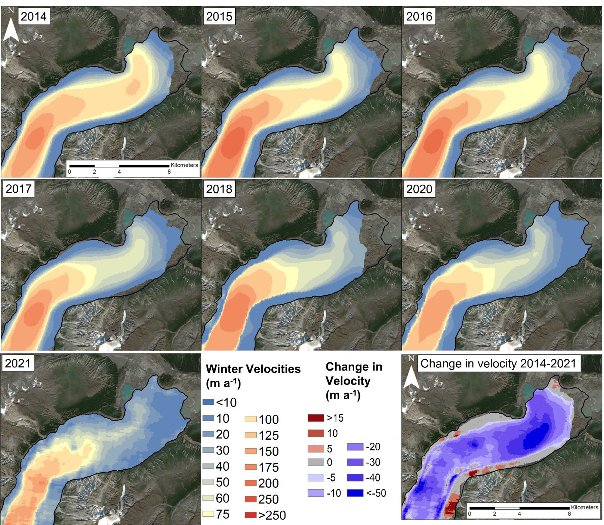
Fig. 7. Surface velocities across the terminus of Kaskawulsh Glacier for each winter from 2014–2021 derived from SAR speckle tracking, together with the long-term change in velocity from 2014–2021. The change in velocity was calculated on a cell-by-cell basis using Cell Statistics tool in ArcGIS between the 2014/2015 and 2020/2021 mean. Note different scale for positive vs negative changes. Projection: UTM 7N, base image: Sentinel-2, August 3 2019.
The terminus of Kaskawulsh Glacier has lost substantial thickness since 1899, with the ice surface sitting approximately 227 m lower at the western edge of the glacier at location I (Fig. 1) in 2020 compared to 1899/1900, with a range of ice loss from 186 to 279 m. Thinning rates have been particularly high over the past two decades, with losses exceeding 70 m at some locations across the terminus between 2003 and 2020 (Fig. 8). The mean total surface elevation loss from 2003–20 was 26.6 ± 1.7 m, or 1.56 m a−1 over the terminus region as a whole. The loss was greatest for the south (Kaskawulsh Lake) lobe, thinning at an average rate of 2.1 ± 0.1 m a−1, compared to the north (Slims Lake) lobe at 1.1 ± 0.1 m a−1 (Fig. 8).

Fig. 8. Elevation change across the terminus of Kaskawulsh Glacier between 2003 and 2020, clipped to the 2020 glacier outline. The black 2020 polygon delineates the terminus region, where a total ice loss value was calculated. Projection: UTM 7N, base image: Sentinel-2, August 3 2019.
Elevation change profiles along the H-H′ cross-section (Fig. 1), ~6.5 km up-glacier from the terminus (Fig. 9a), also demonstrate a marked reduction in glacier surface height from 2003–20. Losses at this location have been most pronounced along the north (Slims Lake) side, with average elevation loss of 22 ± 1.7 m (1.3 m a−1) north of the medial moraine on H-H′. On the south side of the medial moraine the average elevation loss was 13.3 ± 1.7 m (0.78 m a−1). The I-I′ cross-section (Fig. 9b), which is within 2.5 to 4 km from the terminus, experienced a loss of 25–30 m (1.47–1.76 m a−1) across most of the glacier from 2003–20, aside from a narrow region of elevation increase north of the medial moraine.

4.4 Terminus velocities
A comparison of the glacier velocities derived from the dGPS record and RADARSAT-2 speckle-tracking for the same dates found generally strong agreement between the two methods, in terms of both magnitude and direction of motion (Fig. 10). The RADARSAT-2 velocities were often slightly lower than the point velocities derived from the dGPS station, likely due to the ~500 m averaging area that the speckle-tracking velocities are derived from. However, the magnitudes only varied by <10% between the methods and the relationships were all highly statistically significant at p < 0.001.

Fig. 10. Comparison of RADARSAT-2 derived ice motion (a) magnitude and (b) direction values with in-situ velocities from the Kaskawulsh dGPS Station (location shown in Fig. 1). Solid blue line shows the 1:1 relationship between the two measurement methods.
Long-term (1995–2018) annual velocities from the ITS_LIVE dataset point to variations which occur over multi-year periods, particularly for the north lobe (Fig. 11a) compared to the south (Fig. 11b). For the north lobe, highest velocities occurred a distance of 8–10 km from the terminus. From 1995–99, glacier velocities at this location for the north lobe reduced from ~120 to ~90 m a−1, then increased through the 2000's, peaking in 2012 at ~160 m a−1, after which they dropped from ~155 m a−1 in 2015 to ~120 m a−1 in 2018. While the velocity signal is dominated by the high velocities up-glacier, there is also a clear signal in the lowermost ~3 km of the terminus, where average velocities ranged from a low of ~20 m a−1 in 1998/1999, and increased dramatically through the 2000's to a peak of ~125 m a−1 in 2013. They then decreased from 105 m a−1 in 2015 to 55 m a−1 in 2018, a 48% loss at a rate of 12.5 m a−2. While the south lobe exhibits a weaker signal (Fig. 11b), average glacier velocities followed a similar pattern to the north lobe.

Fig. 11. Annual average velocity profiles in m a−1 created from ITS_LIVE data along the (a) north and (b) south lobe centrelines of Kaskawulsh Glacier, 1995–2018. See Figure 1 for location of centrelines and distance markers.
From the detailed patterns provided by the RADARSAT-2 data since 2014 it is clear that the north and south lobes behaved differently (Fig. 7), with the centerline profiles indicating that the north lobe experienced the largest velocity changes at ~3 km up-glacier from the terminus (Fig. 12a). Velocities decreased from ~100 m a−1 in 2014–2015, to 75 m a−1 in 2016–2017 and finally to 50 m a−1 in 2017–2021. The south lobe experienced the largest change in velocities at 5–7 km up-glacier from the terminus, where they decreased from ~100 m a−1 in 2014, to ~75 m a−1 in 2015/16, 50 m a−1 in 2017 and finally to 25 m a−1 in 2021 (Fig. 12b). Velocity data in 2021 is more noisy than other years due to the change in data source from RADARSAT-2 to RCM, and associated change in spatial resolution and reduction in number of scenes available for averaging (Table S4).

Fig. 12. Velocity profiles in m a−1 derived from speckle-tracking of Radarsat-2 data for centrelines along the (a) north and (b) south lobes of Kaskawulsh Glacier, 2014–2021. Cross-profiles of velocity measurements in m a−1 at cross-profiles (c) G-G′, (d) H-H′ and (e) I-I′ on Kaskawulsh Glacier from 2014–2021. Locations for all centrelines, cross-profiles and distance markers are shown in Figure 1.
At the cross-profiles since 2014, velocities are consistently higher up-glacier near cross-profile G-G′ (16–18 km up-glacier from the terminus; Fig. 12c), and have shown little recent slowdown. In comparison, velocities at profiles H-H′ and I-I′ (within 7 km of the terminus; Figs 12d, 12e) are lower and have slowed dramatically over 2014–2021, with the highest velocities decreasing from ~90 to 50 m a−1 near the glacier centreline, and to near stagnation at the glacier margins.
4.5 Terminus floatation
Comparison of the ratio of ice thickness to water depth in 2015, 2016 and 2021 allowed for determination of the location of terminus flotation along line A-A′ to be calculated for these years (Fig. 13a; with ranges provided for 2015 and 2016 to account for the variability in ice thinning of 1 to 2 m a−1 (Young and others, Reference Young, Flowers, Berthier and Latto2020) compared to the 2021 ice thickness measurements). In 2015, both the high and low estimates for floatation were below 0, which indicates that the ice was floating for the lowermost ~350 m of the terminus as it entered Slims Lake. In contrast, after the drainage of Slims Lake in May 2016, no section of the terminus was floating in summer 2016, with 0.8 to 10.1 m of ice loss needed to induce floatation over the lowermost ~200 m at that time. In 2021 there was also no evidence of floatation, with at least 2.7 m of thinning required to induce floatation over the lowermost 27 m of the terminus, and more needed up-glacier of there.

Fig. 13. (a) Ice in excess of floatation at Kaskawulsh Glacier terminus in 2015, 2016 and 2021, along a section of radar line A-A′ (see Fig. 4a for ice thicknesses). The vertical dashes represent the terminus extent for 2015 (coral), 2016 (green) and 2021 (dark blue). (b) Zone of likely floatation at the terminus of Kaskawulsh Glacier as it entered Slims Lake in 2015, based on ice surface elevation and presence of water-filled crevasses in RapidEye-3 imagery. Projection: UTM 7N; base image: RapidEye-3, 8 September 2015.
Figure 13b indicates the region of the terminus that was likely floating, based on extrapolation of the 2015 floatation zone along line A-A′ and ice surface elevation contours, verified with the presence of water-filled crevasses and ponded water on the glacier surface in 5 m resolution RapidEye-3 imagery from September 8, 2015. This region accounts for the upper range in surface melt in Figure 13a and covers an area of 1.13 km2, extending ~100 to 800 m inland from the terminus. In addition, the presence of large, tabular icebergs in Slims Lake are indicative of a floating terminus, as this is the condition typically required to produce these features.
5. Discussion
5.1 Long-term changes in terminus position
The long-term photographic record highlighted in this study (Figs 2, 3) demonstrates that Kaskawulsh Glacier was still near its Little Ice Age maximum extent in 1899/1900. Previously, Borns and Goldthwait (Reference Borns and Goldthwait1966) suggested that the glacier began advancing in the 1500s, reaching its maximum Little Ice Age (LIA) limit by ~1690. However, radiocarbon dating of tree fragments in the outermost terminal moraine by Reyes and others (Reference Reyes, Luckman, Smith, Clague and Van Dorp2006) place the timing of maximum extent from 1717–1750. Their outline represents the maximum LIA extent of the glacier, with the north (Slims Lake) lobe dated to the mid-1750s, and the southern (Kaskawulsh Lake) lobe to 1717. The relative proximity of the 1899/1900 terminus position to the 1717/1750 moraines, along with a Geological Survey of Canada map of the glacier terminus from 1900 to 1904 (McConnell, Reference McConnell1905; see Fig. 2a in Flowers and others, Reference Flowers, Copland and Schoof2014) indicate that there were only minor changes in the terminus position of Kaskawulsh Glacier from ~1750 until the start of the 20th century. The expansion of Kaskawulsh Glacier occurred concurrently with that of the coastal Gulf of Alaska glaciers, which reached their LIA maximum extent (or maintained their maximal positions) from 1790–1900 (Gaglioti and others, Reference Gaglioti2019).
Kaskawulsh Glacier has been retreating since the beginning of the 20th century, with rates increasing since the start of the 21st century (Fig. 5). The glacier has been experiencing long-term thinning in the terminus region compared to the LIA maximum extent, with estimated ice thickness loss from 1899 to 2021 ranging from 186 to 279 m, with an average of 227 m, based on a comparison of ice-free DEMs with 1899/1900 terminus extent along bedrock outcrops (i.e., ice marginal locations in Figs 2, 3). The total volume loss of the terminus from 2003–20 (extent of black polygon in Fig. 8) was 0.38 ± 0.005 km3, at a mean thinning rate of 1.56 m a−1, equivalent to 0.35 ± 0.005 Gt of ice. The formation of substantial proglacial lakes occurred at Kaskawulsh Glacier between 1900 and 1956, as they were not present in the 1899 or 1900 historical photos (Figs 2a, 3a). There was significant growth in Slims Lake after 1990, when it had drained completely, to a maximum of 3.6 ± 0.2 km2 in 2015. Lake area grew steadily from 1995–2009, varied little between 2010–14, and then increased sharply in 2015 before draining in 2016 (Fig. 6). The size and location of Kaskawulsh and Slims lakes have evolved (Fig. 6a) simultaneously with terminus retreat (Fig 5), with the lakes growing and changing location to occupy regions previously covered by glacier ice. This glacier-lake evolution has also been observed across the Southern Alps in New Zealand, as demonstrated by Carrivick and others (Reference Carrivick2022).
5.2 Long-term changes in terminus velocity
The velocity patterns indicate that ice flow at the terminus is dominated by the north lobe (Figs 7, 11), which flows into Slims Lake, compared to the south lobe, which terminates in Kaskawulsh Lake. This velocity pattern has been evident since the mid-1990s, and along with ice thickness observations (Fig. 4a), indicates that significantly more ice is funnelled through the north lobe towards Slims Lake, whereas the south lobe has been relatively stagnant in comparison.
Borns and Goldthwait (Reference Borns and Goldthwait1966) estimated glacier velocity near the terminus to be ~215 m a−1 for 1953–55, although the exact location is not known, precluding any detailed comparisons with our measurements. Waechter and others (Reference Waechter, Copland and Herdes2015) reported a peak winter velocity at cross-profile H-H′ of approximately 180 m a−1 in 1987–88, 60 m a−1 in 1997–98 and 80 m a−1 in 2011–12, which align with the winter RADARSAT-2 velocities reported here (Fig. 7). Average annual ITS_LIVE velocities decreased at H-H′ and I-I′ from 1995–99, from ~45 to ~20 m a−1 and ~30 to 15 m a−1, respectively (Fig. 6b). From 2000–13, average velocities increased at cross-profile H-H′ from ~25 to ~75 m a−1 and at I-I′ from ~20 to ~70 m a−1. The highest velocities observed at both H-H′ and I-I′ occurred in 2013, at ~135 m a−1.
To understand the drivers of more recent changes of the velocity of the north lobe, analyses were undertaken of the relationship between the mean velocity at profiles G-G′, H-H′ and I-I′ and the changes in area of Slims Lake (Supplementary material, Fig. S1). R 2 values demonstrate that ~30% of the variance of the combined winter and annual average velocities at H-H′ and I-I′ is explained by Slims Lake area (p < 0.05), while the relationship at G-G′ is not significant. More variability is explained when average winter velocities are excluded (~50 and ~40%, for H-H′ and I-I′, respectively) (Fig. S1). This indicates that there is a relationship between changing ice velocities and Slims Lake extent close to the terminus, whereas up-glacier the influence of the lake size is minimal, and that this relationship is significant only when considering annual average velocities.
5.3 Rapid change in velocity after 2016 Slims Lake drainage and loss of floatation
Analysis of velocities over the 5-year periods before (2010–15), and after (2016–21), the Slims Lake drainage for each of the terminus lobes are shown in Table S5. Pre-drainage (2010–15) there was no significant change in velocity change for either lobe, nor within the combined terminus region. After the 2016 drainage, there was a statistically significant slowdown (p ≤ 0.05) across the terminus at a mean rate of 3.5 m a−2, with the slowdown dominated by the north lobe, decreasing at 4.0 m a−2 compared to the south lobe decreasing by 2.9 m a−2.
Our analysis shows that, while Kaskawulsh Glacier winter velocities have been slowing prior to the May 2016 proglacial lake drainage, the velocity decreased markedly after 2016 to a low of <50 m a−1 in 2021 (Fig. 12b). The effect is most pronounced over the lower 5 km of the north lobe terminus, where velocities decreased from ~75 to <50 m a−1, a 33% decrease. Annual average ITS_LIVE velocities (Fig. 11), while temporally limited up to 2018, indicate a similar drop in velocities from ~100 m a−1 in 2015, to ~60 m a−1 in 2018 within 5 km of the terminus, a 41% loss. From 5–10 km up-glacier, the signal is weaker, where velocities decreased from ~130 m a−1 in 2015 to 100 m a−1 in 2018, a 22% deceleration. This indicates that the effect of the proglacial lake might be localised, as beyond ~7 km up-glacier from the terminus the friction from the valley sides and the distance from the floating section can limit any additional dynamic thinning and acceleration.
The floatation data (Fig. 13) suggests that the last 325 to 375 m of the glacier terminus was floating in 2015, but that floatation has not occurred since then despite continued retreat, an increase in the lake size, and continued ice thinning. This suggests that the May 2016 drainage event and associated loss of floatation was a primary driver of the recent reductions in velocity across the glacier terminus, in combination with the ongoing reduction in ice thickness due to surface melt.
5.4 Lake theory: hydrology and flow dynamics
An additional possible driver slowing ice flow following lake drainage is adjustments to the basal hydrology. Channels form at the base of glaciers when there is a strong gradient in hydraulic potential which allows sufficiently fast water flow to melt the overlying ice (Röthlisberger, Reference Röthlisberger1972; Shreve, Reference Shreve1972). This is influenced by the baseline or outlet potential; when a lake is present that is floating the terminus of a glacier, the outlet hydraulic potential is the same as the ice overburden pressure. However, when that lake drains, the outlet pressure is atmospheric, immediately steepening the hydraulic gradient. The change in gradient would encourage faster water flow underneath the ice and therefore growth of larger and more efficient channels that can become lower pressure, and can draw more water from the distributed subglacial system, slowing down the ice further (Fountain and Walder, Reference Fountain and Walder1998).
If we take the ice thickness and surface elevation from near the centreline along radar line A-A′, and from near the terminus along radar line B-B′, we can calculate the hydraulic potential for both a full lake and drained lake scenario. We use the Shreve (Reference Shreve1972) hydraulic potential equations with the assumption that water pressure underneath the ice is at overburden pressure:

where ρw is the density of water (1000 kg m−3), ρi is the density of ice (917 kg m−3), g is the acceleration due to gravity (9.81 m s−2), z is the elevation of the bed (m), and H is the ice thickness (m). We calculate the average gradient of hydraulic potential using the following:

where z1 and H1 are the basal and ice thickness values (m) at the upper site, z2 is the basal elevation (m) at the terminus, D is the distance between the upper site and terminus (m), and Pw2 is the outlet water pressure either at overburden pressure (if the lake is full) or 0 if the lake is empty. This gives a value of 339.7 Pa m−1 when the lake is full and 440.6 Pa m−1 when the lake is empty, demonstrating a significant increase in hydraulic potential gradient that would directly impact flow rates of subglacial water. Even when water is at pressures lower than overburden, depending on the volumes entering the system, the change in hydraulic gradient will impact the rates that water flow to the outlet at atmospheric pressure.
Longitudinal stretching is another process which may have been influenced by the growth of Slims Lake (Fig. 6) as the glacier terminus thinned (Figs 8, 9) and the ice started to float (Fig. 13). When floatation occurs, there is a reduction in basal friction and increased velocities cause thinning to propagate up-glacier (Benn and Evans, Reference Benn and Evans2010). This can also impact subglacial hydrology by reducing the overburden pressure and steepening the hydraulic gradient. This process was documented at Glaciar Upsala, in Southern Patagonia, where, once floatation and enhanced basal sliding was induced, longitudinal stretching rates reached 0.22 a−1 (Naruse and Skvarca, Reference Naruse and Skvarca2000); as well as at Yakutat Glacier, Alaska, where 17% of total ice thinning was attributed to dynamic thinning from 2007–10 (Trüssel and others, Reference Trüssel, Motyka, Truffer and Larsen2013). A dGPS study in the Himalaya found that ice thickness loss was 3 times greater for a lake-terminating glacier compared to land-terminating, with numerical modelling indicating that this was driven by dynamically induced ice thinning along with a negative surface mass balance (Tsutaki and others, Reference Tsutaki2019). Similarly, Pronk and others (Reference Pronk, Bolch, King, Wouters and Benn2021) found that ~50% of the lake-terminating glaciers in their study area experienced a velocity acceleration towards the glacier termini, which they attributed to dynamic thinning.
Thinner ice is more easily able to crevasse and to calve into a lake, thus increasing terminus retreat and allowing Slims Lake to grow (Warren and Kirkbride, Reference Warren and Kirkbride2003; Benn and others, Reference Benn, Warren and Mottram2007; Tsutaki and others, Reference Tsutaki2019). During the 2000–15 period of lake growth and velocity acceleration, crevassing at the terminus increased in both intensity and extent (Fig. S2). The frequent presence of large, tabular icebergs in Slims Lake suggests that calving is a more common process at the north lobe terminus, compared to the south lobe at Kaskawulsh Lake, where significantly fewer and much smaller icebergs are observed, and the ice is much thinner (Fig. 4a). This increase in longitudinal drag pulls ice at an accelerated rate from upstream until friction from the valley walls and the distance from the floating segment mitigate the additional dynamic thinning and acceleration (~5 km from glacier terminus), thus limiting the impact on up-glacier velocities.
The presence of a reverse bed slope (Fig. 4a), particularly over the northern portion of the terminus, indicates that as Kaskawulsh Glacier continues to retreat (up to 23 km as suggested by Young and others, Reference Young, Flowers, Berthier and Latto2020), deeper topography will be exposed. While a substantial portion of Slims Lake drained in 2016, it has started to grow again, and it will continue expanding as it infills exposed space vacated by retreat. Schoof (Reference Schoof2007) has shown that steady grounding lines cannot be stable on reverse bed slopes because retreat into deeper water enhances ice flux, promoting additional terminus recession; however, Schoof's study does not account for lateral support, such as from valley walls, which may impact the degree of instability and be an influence for Kaskawulsh Glacier. As Slims Lake expands into the exposed trough, it will become easier for floatation to occur, which may cause velocities to increase, and for the grounding line to rapidly retreat (Sutherland and others, Reference Sutherland2020). For example, rises in bedrock topography were found to strongly control glacier terminus fluctuations at Glaciar Upsala, Argentina (Naruse and Skvarca, Reference Naruse and Skvarca2000). Field and others (Reference Field, Armstrong and Huss2021) also suggest that proglacial lake geometry and topographic setting (e.g., the ability for the surrounding basin to accommodate lake growth, as is possible under a reverse-slope regime) exert a key influence on glacier stability.
5.5 Comparisons with velocity changes at other proglacial lakes
The influence of proglacial lakes on glacier terminus velocities and glacier dynamics have previously been examined in locations such as Switzerland, New Zealand, Nepal and Iceland (Tsutaki and others, Reference Tsutaki, Sugiyama, Nishimura and Funk2013; Haritashya and others, Reference Haritashya, Pleasants and Copland2015; Baurley and others, Reference Baurley, Robson and Hart2020). For example, Robertson and others (Reference Robertson, Brook, Holt, Fuller and Benn2013) found that an increase in the size of a proglacial lake adjacent to Hooker Glacier, New Zealand, occurred simultaneously with an increase in terminus retreat, as ablation changed from melting to calving. Modelling of Yakutat Glacier found that while proglacial lake presence has a substantial immediate influence on glacier retreat rates via calving, this is subsequently compensated for through an increase in surface melt, leading to near-equal glacier volume loss over time (Trüssel and others, 2015). Haritashya and others (Reference Haritashya, Pleasants and Copland2015) reported that the lowermost ~3 km of Tasman Glacier, New Zealand, experienced a steady acceleration from near-stagnation to 40–50 m a−1 during the 2000's which coincided with the rapid growth of a proglacial lake, while a study of Rhonegletscher, Switzerland also demonstrated an increase in annual velocity by a factor of 2.7 at the glacier terminus during the formation of a proglacial lake over a 5-year period (Tsutaki and others, Reference Tsutaki, Sugiyama, Nishimura and Funk2013). In the central and eastern Himalaya, Pronk and others (Reference Pronk, Bolch, King, Wouters and Benn2021) found that velocities of land-terminating glaciers were on average less than half those of lake-terminating glaciers.
Numerical modelling has suggested that the presence of a proglacial lake caused the glacier to retreat more than 4 times further up-glacier, and ice acceleration 8 times higher, compared to the modelled glacier with the same climatic parameters terminating on land (Sutherland and others, Reference Sutherland2020). In simulations of Pukaki Glacier in New Zealand, lake presence contributed up to 82% of the grounding line recession and 87% of ice velocity for the first 5000 years before influence declined, suggesting that the largest impact on glacier dynamics is during the transition between a land-terminating and lake-terminating environment (Sutherland and others, Reference Sutherland2020). The relationship between proglacial lake size and glacier velocities is more moderate at Kaskawulsh Glacier compared to those predicted by numerical modelling, possibly due to complicating environmental/structural factors including the irregular bed shape and additional proglacial lake. Regardless, this study provides a basis to investigate further the implications of increasing proglacial lake size on glacier dynamics.
6. Conclusions
This study has extended the photographic record of Kaskawulsh terminus changes to 120 years, almost doubling the length of the previous record of Foy and others (Reference Foy, Copland, Zdanowicz, Demuth and Hopkinson2011), demonstrating that terminus retreat since the end of the LIA continues, but has been increasing in recent years. The glacier has experienced fluctuations in annual and wintertime average velocities from 1995–2021, but two main trends are common between the velocity datasets. From 2000–15, annual average glacier velocities increased at a rate of ~5.5 m a−2, while from 2010–15 average winter velocities increased by ~2 m a−2. Associated with increasing velocities was the expansion of proglacial Slims Lake at the northern terminus, from ~0.2 km2 in 1995 to ~3.6 km2 in 2015. The spring 2016 drainage of Slims Lake instigated a major reduction in both winter and annual average terminus velocities through a loss of floatation along the northern terminus. Average winter velocities decreased at a rate of ~3.5 m a−2 from 2016–21 across the terminus zone, dominated by reductions in the northern lobe. From 2016–18, annual average velocities along the lowermost ~10 km of both the north and south glacier centrelines (Fig. 1) decreased by ~8 m a−1. Approximately 45% of the change in annual average velocity is explained by the size of Slims Lake. Glacier velocities were mainly influenced within ~7 km of the glacier terminus, suggesting a localised control on glacier dynamics, although further studies are needed to understand if these controls will impact up-glacier velocities over time.
Although the 2016 drainage of Slims Lake ended terminus floatation and locally reduced glacier velocities, the probability of a new, even larger, lake forming is high as the glacier enters a reverse bed slope regime through continued terminus retreat (Young and others, Reference Young, Flowers, Berthier and Latto2020). As such, this scenario provides an opportunity to further study the projected retreat of Kaskawulsh Glacier and its application to glacier dynamics. Representing the mid-point on the climate sensitivity continuum between least-sensitive (tidewater glaciers) to highest sensitivity (land-terminating glaciers) (Warren and Kirkbride, Reference Warren and Kirkbride2003), the impacts of various factors on lake-terminating glaciers are not yet fully understood and require further examination. Such linkages will likely be of increased importance in the coming decades as it has been hypothesised that there may be an increase in proglacial lake formation with climate warming (Zhang and others, Reference Zhang, Yao, Xie, Wang and Yang2015; Cook and others, Reference Cook, Kougkoulos, Edwards, Dortch and Hofmann2016; Furian and others, Reference Furian, Maussion and Schneider2022).
Supplementary material
The supplementary material for this article can be found at https://doi.org/10.1017/jog.2022.114
Data
The photogrammetry dataset (DEM and Orthomosaic) generated for this study, together with our RADARSAT-2 wintertime glacier velocities, are available from the Polar Data Catalogue (https://polardata.ca/) under CCIN reference numbers 13285 and 13292, respectively. Original RADARSAT-2 data is available through MDA Geospatial Services (https://www.asc-csa.gc.ca/eng/satellites/radarsat2/order-contact.asp). Historical terrestrial photos are available from the Mountain Legacy Project website (https://mountainlegacy.ca). All satellite imagery (Landsat, Sentinel-2 and ASTER), air photos, and ITS_LIVE annual velocity mosaics are publicly available from data sources listed in the methods.
Acknowledgements
We thank Kluane First Nation and Parks Canada for permission to undertake field measurements at Kaskawulsh Glacier. Support for this research has been provided by the University of Ottawa, Natural Resources Canada (Canada Centre for Earth Observation and Mapping), the Northern Scientific Training Program, the Canadian Space Agency (Radarsat Constellation Mission Data Utilization and Application Plan), Montana State University, NSERC, the Weston Family Foundation, Canada Foundation for Innovation, Ontario Research Fund, Parks Canada, Kluane Lake Research Station and Polar Continental Shelf Program. Support for travel to conferences and attendance of courses was generously provided by the ArcticNet Network of Centres of Excellence Canada Student Training Fund, GlacioEx and RemoteEx. We thank the Mountain Legacy Project and Library and Archives Canada / Bibliothèque et Archives Canada for providing the historical imagery. We are grateful for the thoughtful and constructive comments provided by editor L. Andreassen, and by reviewers M. Truffer and J. Sutherland.
Author contributions
BM and LC designed the study. BM processed the velocity/lake datasets, completed the analysis and wrote the initial draft of the manuscript with input from LC, MS, CD, WVW and WK. SS, JD, CD, LM, WK, DM, BS, EH and WVW all provided processed datasets. All authors revised the paper prior to submission.


 Open access