Nomenclature

• a _s Specific surface of the snow

• C _p Specific heat

• D _a Diffusivity of water vapor in air

• D _s Diffusivity of water vapor in snow

• d _p Particle diameter

• h _m Mass-transfer coefficient for vapor

• J _i Vapor flux i-direction

• k _ij Permeability of snow

• L _v Latent heat of vaporization

• Ρ Pressure

• Q _T Source term in temperature equation

• S Source term for vapor density

• Τ Temperature

• t Time

• ʋ Characteristic velocity of air flow through snow

• ʋ _i Darcy velocity in i-direction

• x _i Coordinate direction, i = 1,2,3

Greek Symbols

• α Ratio of the diffusivity of water vapor in snow to that in air

• φ Porosity

• λ Thermal conductivity

• ρ Density

• μ Molecular viscosity

• ν Kinematic viscosity

Subscripts

• a Air

• h High

• i Ice

• l Low

• m Matrix

• o Reference value

• s Snow

• v Vapor

Superscript

• s Saturated

Dimensionless Numbers

• Pe Peclet number

• Re Reynolds number

• Sc Schmidt number

• St Stanton number

Introduction

The study of macroscopic heat and mass transfer through snow has important applications in infrared thermography, snow hydrology and contaminant transport. In this paper we consider the heat-transfer effects associated with the flow of air and the transport of water vapor through dry snow. In Nature, air movement through snow may occur as free convection, where the driving force is temperature gradient, or as forced convection, where the driving force is pressure gradient. Studies have illustrated that free convection, sometimes termed natural convection, may sometimes occur in snow; when it occurs, it has the effect of enhanced heat transfer within the snow (Reference Powers, Colbeck and O’NeillPowers and others, 1985; Reference Sturm and JohnsonSturm and Johnson, 1991). There have been field and analytical studies (Reference ReimerReimer, 1980; Reference Clarke, Fisher and WaddingtonClarke and others, 1987; Reference ColbeckColbeck, 1989; Reference Clarke and WaddingtonClarke and Waddington, 1991; Reference Albert and McGilvaryAlbert and McGilvary, 1991) which note possible effects of forced convection, e.g. that there sometimes occurs a significant disruption in the thermal regime of the snow when windy conditions prevail, an effect sometimes termed windpumping. Thus, it is possible that both free and forced convection may occur in Nature. It is the forced flow of air through seasonal snow covers that motivates the investigation presented here.

Several laboratory studies have been conducted on ventilation of snow. (Reference Yen Yin-Chao.Yen 1962, Reference Yen Yin-Chao.1963) reported on laboratory experiments where air saturated with vapor was forced through a column of snow subjected to an imposed temperature gradient. While the experimental results are interesting, the results were lumped into “effective” parameters that confounded effects of convection and conduction; important differences in the physics of diffusion and convection were ignored in the presentation of results. Reference Sackly and LambrinosSackly and Lambrinos (1989) documented experiments on global mass transfer associated with air flow around (and presumably through) a cylindrical snow sample. They presented a mass-transfer coefficient that is valid for snow cylinders in cross flow, but unfortunately will not be adequate for air-circulation patterns within the snow.

This paper has two objectives. The first is to describe a theory for predicting macroscopic thermal effects associated with the advection of heat and vapor by air movement through snow, including the possibility that the snow is not saturated with vapor. Previous analyses of thermal processes in snow (e.g. Reference AndersonAnderson, 1976; Reference Powers, Colbeck and O’NeillPowers and others, 1985) have assumed saturated vapor conditions in the snow. The present analysis is new in that we allow the air in the snow to be supersaturated, saturated or unsaturated with vapor; thus, we account for the effects of sublimation.

The second objective is to examine, for air flow through snow, the heat-transfer roles played by the sensible heat transferred by conduction and advection, and the latent heat associated with sublimation and condensation. We seek to clarify the magnitude of the effect of each phenomenon in determination of the final temperature profiles, and for this paper we focus on the simple case of the ventilation of a snow sample subject to fixed temperatures at the boundaries of the sample. It is our objective to examine each of the important effects in a comprehensive theory, and then to isolate each effect to determine its importance in the overall problem. This approach differs markedly from many snow thermal models developed in the past, which lumped physical effects through the use of “effective” parameters. In the process of developing our theory, we make note of experiments that will be necessary for determination of some of the parameters involved.

In the following sections, we detail the mathematical theory for this heat-, mass-and momentum-transfer problem. The equations necessary to calculate forced air flow through snow, the transport of vapor through snow and the associated heat transfer with each are detailed. The resulting set of coupled, non-linear partial differential equations is solved numerically using the finite-element method. We compare the results of the numerical solutions with analytical and experimental results. We use the model to investigate and isolate the various thermal effects incurred by the forced convection of air through the snow sample. Finally, we generalize the results and discuss their implication for the thermal effects of windpumping in snow.

Governing Equations

Air Flow

The equations for forced flow of air through a porous medium are first presented. The dry air is treated as an incompressible medium, where conservation of mass follows

(1)

where x _i is a coordinate direction (i = 1,2,3). Repeated indices imply summation over three orthogonal directions. For cases considered here of flow through an unconstrained sample in the absence of shocks, compressibility effects are negligible. Viscous dissipation effects will also be negligible, since the heat loss due to viscous shear in an incompressible laminar flow is equal to the flow rate times the pressure change (Reference Streeter and WylieStreeter and Wylie, 1979). This heat loss is several orders of magnitude below the conductive-and advective-heat fluxes considered here.

The air flow is assumed to follow Darcy‘s law, where the Darcy velocity or volumetric flux of the air, ʋ_i, is given by

(2)

where buoyancy effects are neglected, Ρ is pressure, k_ij is permeability and μ is viscosity. By combining Equations (1) and (2), the single equation to be solved for the air flow is

(3)

Vapor Transport

The theory incorporated in past snow thermal models assumes that the local vapor density in the snow is equal to the saturation density at the local snow temperature. The development which follows represents the first treatment of snow which is not limited by that assumption. The transport of water vapor through snow is described by the advection-diffusion equation:

(4)

where the source term, S, is the source of vapor due to sublimation or condensation. It is evident from the equation that the vapor density at a given location may change in time due to advection of vapor by the air flow, diffusion of vapor by vapor-density gradients and generation or dissipation of vapor by the source term. Since the vapor density is small compared to the density of the air, the advection term assumes that the vapor is carried by the air flow.

Because this is a new method for determining the effects of vapor transport, we will discuss in detail some of the parameters and terms in Equation (4). Following mass-transfer theory, the diffusion coefficient for water vapor in snow is assumed to be proportional to the diffusion coefficient in air:

(5)

For non-reactive materials, α is the ratio of porosity to tortuousity (Reference Sherwood, Pigford and WilkeSherwood and others, 1975), in which case α is less than one. However, because the ice matrix of snow reacts with water vapor, it has been found (e.g. Reference YosidaYosida, 1955; Colbeck, 1991) that α for snow may lie between 4 and 7. There is uncertainty in the determination of α for snow; clearly this is an area which warrants further study.

For both heat and mass transfer, the source term, S, in Equation (4) is an important quantity and requires explanation. The source of vapor responds to sublimation which is driven by two phenomena: a change in vapor concentration due to the diffusion of vapor which is induced by temperature gradients alone, and a change in vapor concentration due to the advection of vapor by air flow through the pore space. The theory presented here includes both phenomena, although the primary concern of this paper concerns situations involving significant air flow.

It is well known that the flow of a fluid or gas through a medium results in mass-transfer rates that can be considerably higher than those which occur by diffusion alone. We describe the source of vapor due to phase change enhanced by air flow through the snow by

(6)

The specific surface of the snow, α_s, is the surface area of the ice matrix per unit volume of snow. The saturation vapor density, ρ_v ^s, is given by the following curve fit to psychrometric data (Reference AshraeASHRAE, 1989), which takes on the form of the Clausius–Clapeyron equation of state:

(7)

where ρ _v0 and T ₀ are reference vapor density and temperature, respectively, and C₁ = 6145 K. Technically, the saturation vapor density varies with both the mean radius of curvature of the ice-vapor interface and with temperature gradient; however, the temperature effect dominates (Reference ColbeckColbeck, 1982), and we neglect curvature effects in this macroscopic model.

The mass-transfer coefficient in Equation (6), h _m, has not yet been determined for snow, and the authors plan to conduct laboratory studies for the determination of this parameter. In the absence of data on snow, we employ a correlation of Reynolds, Schmidt and Stanton numbers developed by Reference Chu, Kalil and WetterothChu and others (1953) for mass transfer in gas-solid and liquid-solid systems in fixed and fluidized beds of porous media for spherical and cylindrical particles. This correlation was derived from a wide variety of materials and particle sizes:

(8)

where the Stanton number is St = h _mϕ/ν, the Reynolds number is defined by Re = d _pυ/v_a (1 − ϕ), the Schmidt number is Sc = v _a/D _a porosity is ϕ = 1 − (ρ_s/ρ_i), d _p is the particle diameter, v _a is the kinematic viscosity of air (1.596 × 10⁻⁵ Ν s m⁻¹), ρ is density, and subscripts s and i denote snow and ice, respectively. This correlation was developed by those with an interest in optimizing mass transfer, and was determined from data on many materials and Reynolds numbers between 1 and 30. The Reynolds number for correlation (8) is plotted as a function of air velocity, with snow type as a parameter, in Figure 1. Note that the above definition of Reynolds number includes porosity in the denominator, unlike the usual convention for Darcy flow. Reference BearBear (1972) indicated that Darcy‘s law is valid so long as the ratio d _pυ/υ_a does not exceed “some value between 1 and 10”. Then correlation (8) holds at least for flow velocities which fall in the upper regions of the Darcy-flow regime. For higher flow rates, one would replace the Darcy flow Equation (3) by an equation including inertial effects. Correlation (8) holds for the velocities investigated in the present work.

Fig. 1. Reynolds number versus air velocity for five snow types.

We hypothesize that correlation (8) may be valid for lower air-flow velocities, and we take a brief digression to investigate this possibility. For a situation with no air flow, the sublimation process provides a source of vapor that is limited by the rate that diffusion can transfer vapor away from the source. Now, when air flows through the system, vapor is transported away from the source by advection, enabling a higher mass-transfer rate at the source. Since the relationships for advection of vapor presented above might hold down to a flow rate sufficiently low that diffusion dominates, it is possible that correlation (8) may be valid down to a Reynolds number such that the velocity of the vapor movement due to diffusion (“diffusional velocity”) equals that due to advection. From Fick‘s law, the diffusive velocity is

(9)

where ρ_vave is a local average value of the vapor density. Using the results of the simulations of the experimental situations investigated in this paper, diffusive velocities were calculated according to Equation (9), and an upper limit on the diffusive velocities, when inserted into Equation (8), gave mass-transfer coefficients on the order of h _m = 0.09 ms⁻¹. The mass-transfer coefficient given by Equation (8) is plotted as a function of Reynolds number in Figure 2. The horizontal line depicts the mass-transfer coefficient for the diffusive limit as derived above. We believe that the lower limit of applicability of the mass-transfer correlation may lie as low as that line. In that case, the lower limit of applicability of correlation (8) is probably closer to a Reynolds number on the order of 0.2, rather than a Reynolds number of 1. This means that the correlation may be valid for lower air velocities and will thus increase the extent of applicability of the correlation to snow. Further laboratory studies are required in order to verify this hypothesis and to firmly establish h _m for snow.

Fig. 2. Mass-transfer coefficient as a function of Reynolds number.

In the investigations which will be described below, we compare results to published laboratory tests. Because the snow characterization in those tests did not cover some of the parameters required in the analaysis presented here, we are forced to make some basic assumptions about the snow. For the current work, we assume that the snow particles are spheres, and that reported grain-size of snow represents the sphere diameter. The surface area per unit volume of snow may then be obtained from

(10)

In the present analysis, we further assume that α for water vapor in snow is unity, i.e. that the diffusivity of vapor in snow is the same as that in air (2.2 x 10⁻⁵ m s⁻¹). This is acceptable, given the uncertainty in existing data on the diffusivity of vapor in snow, and further warranted because numerical experiments associated with the results presented below showed that the current investigations are not highly sensitive to α.

The mass-transfer coefficient for vapor given by Equation (8) is intended for use when air is flowing through the snow. In Nature, when the air flow in the snow is stagnant, sublimation/condensation mass transfer occurs because of temperature gradients in the snow. The vapor diffuses from warmer snow with a higher vapor density to the lower vapor-density regions in colder snow. To a good approximation, under stagnant conditions, the vapor comes into local equilibrium at each time step. For steady-state solutions this condition is achieved, in the current work, by assigning a high value to the mass-transfer coefficient, h _m, when the velocity of the air is zero. Future laboratory and theoretical work will further investigate effects of situations involving very low air-flow velocities and the matching to higher flow regimes.

Heat Transport

For the prediction of macroscopic heat transfer, the ice-vapor-air system known as snow is assumed to be in local thermal equilibrium. Heat transfer through the snow follows an advective-diffusive equation:

(11)

where

(12)

Here Τ is temperature, C_p is specific heat, λ_ij is thermal conductivity and Q_T is the thermal source term. Equation (12) contains no term involving the vapor because the density of water vapor is much less than that of air, although their heat capacities are similar; thus, we assume that the sensible-heat effects are borne by the air. The source term, Q_T, includes latent-heat effects due to sublimation:

(13)

where S is the vapor source defined in Equation (6) and L is the latent heat (2.83 x 10⁶ J kg⁻¹). For simplicity in the present analysis, we neglect changes in snow density and structure created by phase change.

The coupled set of Equations (3), (4) and (11) are solved on a Vax, using a three-dimensional finite-element code developed by the authors. The code is based on the Galerkin method and uses linear tetrahedral elements. In the following sections we compare the computed results with analytical and experimental results. The method is applicable in three dimensions but a one-dimensional situation serves well for illustrative purposes, and also allows us to compare results with published experimental data. Thus, for the current work, we will focus our attention on one-dimensional investigations.

Comparison with an Analytical Solution

We first consider the case where no air is flowing through the snow. In the absence of air flow, non-linear temperature profiles are expected because of the latent-heat effects due to vapor diffusion through the stagnant medium. In an analytical solution, this may be accommodated in the heat-conduction equation by assigning a temperturc-dependent thermal conductivity. For the case of one-dimensional, steady-state heat conduction subject to constant temperature boundary conditions, a solution is derived (paper in preparation by W. R. McGilvary and M. R. Albert) for the non-linear temperature field. Reference ColbeckColbeck (1982) also derived quasi-linear temperature fields but used constant temperature and vapor-density fluxes at the lower boundary and a constant thermal conductivity. For comparison with analytical results, the air-flow velocity was set to zero in the model, a large mass-transfer coefficient was implemented, and temperature fields were computed for one set of constant temperature boundary conditions for each of two snow types. The input data for both analytical and numerical solutions are detailed in Table 1.

Table 1.

Note that, in the absence of vapor effects, the solutions for these cases are just that of the steady-state heat-conduction equation, which results in a linear temperature profile between the high and low temperatures. The latent-heat effects of vapor make the profiles slightly nonlinear, as depicted in Figure 3a. In Figure 3b, for each case, the departure from the straight-line solution is plotted as a function of location; the solid line is the analytical solution and the symbols denote the computed solution. It is evident from the plots that the analytical and computed solutions show excellent agreement, indicating that the implementation of the mass-transfer coefficient for steady-state, no-flow conditions, is acceptable. It is also evident that the heat transfer due to vapor transport contributes less than 2% to the overall temperature profile as per the infinity norm. (That is, when one compares the temperature profiles due to heat conduction including sublimation to those without sublimation, the maximum temperature difference at any location, divided by the overall temperature difference between the boundaries, is less than 2%.)

Fig. 3. a. Temperature profiles due to heal conduction and vapor transport but no air flow. b. Comparison of analytical and computed results for temperature deviations from linearity due to vapor transport with no air flow.

Comparison with Published Experimental Data

Published data exist for laboratory studies on steady-state, one-dimensional forced air flow through a snow sample subject to fixed temperatures at the air inlet and outlet (Reference Yen Yin-Chao.Yen 1962, Reference Yen Yin-Chao.1963); these laboratory studies were also motivated by field observations of windpumping. A schematic of the experimental situation is depicted in Figure 4. The inlet air is saturated at a fixed, low temperature below freezing, T _in. The outlet temperature is fixed at a higher, but still sub-freezing temperature, T _out. A constant-velocity air flow is maintained through the sample. Since the inlet air is saturated with water vapor, ρ _v at the inlet is known. However, the vapor density (level of saturation) at the outlet was not measured in the laboratory study, and so is not forced to a particular level in the numerical work presented here. (Reference Yen Yin-Chao.Yen 1962, Reference Yen Yin-Chao.1963) reported the resulting steady-state temperature distribution in the snow at several locations along the sample for various flow rates. We will compare the numerical results with those of the laboratory study and also assess what factors most affect the heat transfer in the study.

Fig. 4. Schematic of the experimental and numerical situation.

The situation is modeled by assigning a constant flow velocity throughout. The inlet and outlet temperatures are assigned constant values. The air is saturated with vapor at the inlet but a Neumann boundary condition (zero vapor-density gradient) is assigned to the vapor at the outlet, so that the relative humidity is not forced to a particular value there. A finite-element grid with 400 elements, graduated so that the grid is finer in regions of steeper gradients, is employed. The model was run for two sets of temperature and flow-boundary conditions. The parameters used and details of the boundary conditions for both cases are given in Table 2.

Table 2.

All of the above data except thermal conductivity have been documented in the presentation of experimental results (Reference Yen Yin-Chao.Yen, 1962, Reference Yen Yin-Chao.1963). For the thermal conductivity, we chose values for each density that are the averages of the spread of values for that density listed in Reference MellorMellor (1977). These experimentally determined thermal conductivities already include vapor effects but represent reasonable estimates, since conductivities without vapor effects have not been reported. Figure 5 illustrates the predicted (line) versus measured (symbols) temperature profiles. The model predicts the experimental results to within one-half degree, which is probably within the experimental uncertainty of the determination of the temperatures and inlet saturation of the experiment. This is very good agreement, especially given the uncertainty in the basic parameters such as thermal conductivity. In this situtation, the temperature gradients over the entire sample perhaps seem high relative to those found in Nature. However, the high gradients pose a challenging test of the model and it is believed that the model will perform well when compared to results of upcoming multi-dimensional field tests.

Fig. 5. Comparison of experimental and computed temperatures for two air-flow rates and several values of thermal conductivity.

While the experimental values of thermal conductivity cited above confound the effects of vapor with those of the ice matrix, there is evidently no published determination of the thermal conductivity that separates the two effects. By conducting numerical experiments with varying thermal conductivities, it is possible to determine for these experiments what the thermal conductivity of the ice matrix must have been. This is, in effect, solving the inverse problem using a trial-and-error method. In Figure 5, the predicted temperature distributions with adjusted thermal conductivities are plotted against the experimental results. We see improved agreement between experiment and theory, using thermal conductivities of 0.50 W m⁻¹ K⁻¹ for the snow in case A, and 0.60 W m⁻¹ Κ ⁻¹ for the snow in case B. It is relevant to note that these thermal conductivities, determined by numerical experiment, both lie within the range of conductivities summarized in Reference MellorMellor (1977). We also note that additional improvements in agreement between the model and experimental results for case Β could be had if the inlet temperature were 1/2° higher, or if the inlet air was not exactly at saturation. However, the results show very good agreement and we choose to remain true to the boundary conditions as reported in the experimental work (Reference Yen Yin-Chao.Yen, 1962, Reference Yen Yin-Chao.1963).

In Figure 5 it is evident that the snow near the inlet is nearly isothermal for a significant part of the sample, but that a steep temperature gradient exists closer to the outlet. This is similar to the one-dimensional temperature distributions observed during windpumping events (both during the day and at night) in seasonal snow covers (Reference Jordan and DavisJordan and Davis, 1990), where near-surface temper-atures are nearly isothermal while a steep gradient occurs near the ground, although in the field the air flow probably follows a multi-dimensional pattern. The steep temperature gradients which are forced to occur near the ground in seasonal snow covers cause large vapor transport there, which in Nature may enhance snow metamorphism or growth of depth hoar at that location.

In Figure 6, the calculated vapor density is plotted as a function of location for the two cases, and the relative humidity is also plotted. At the outlet (x = 0.15 m), the relative humidity is 99.2% in case A and 98.7% in case B. It is evident that the incoming cold air had a velocity sufficiently high, and the bottom boundary temperature was sufficiently high, that the air traveled though the sample before it had time to become everywhere completely saturated with vapor.

Fig. 6. Calculated vapor density and relative humidity as a function of location.

Analysis of the Heat-Transfer Effects

We will now isolate the various heat-transfer effects that were present in the experimental investigation, in order to determine the role of each in the comprehensive theory described above.

Heat Conduction Without Vapor Transport

For the two sets of snow properties and temperature boundary conditions listed inTable 2, the model was run with air velocity set to zero and latent heat of sublimation set to zero. The steady-state temperature solutions take the form of straight lines, as depicted in Figure 7. It is clear that heat conduction alone cannot describe the temperature profiles obtained experimentally.

Fig. 7. Temperature profiles obtained with heat conduction without vapor transport.

Air Flow without Vapor Transport

The comparison of model predictions with experimental results in Figure 5 includes both the effects of the latent heat due to vapor transport and the effects of the sensible heat carried by the air. In an effort to separate these effects, the model was also run with heat conduction and advection of heat by the air flow but with no vapor transport. In that case, deviations from a linear temperature profile are due to enthalpy differences of the moving, dry air. With temperature and snow conditions as listed in the comparison with experimental results, Figure 8 depicts the model predictions with and without vapor transport. Although there is a distinguishable difference in the solutions with and without vapor transport, it is obvious that for these snow types, temperature differences, flow velocities and mean temperatures, the sensible heat advected by the air is the controling factor in the resulting temperature regime. In these cases, the heat transport due to sublimation contributes less than 5% to the overall temperature profile, as per the infinity norm.

Fig. 8. Temperature profiles obtained by advection of heat by the air flow, with and without vapor transport.

Generalization and Discussion

The above investigation isolated the effects that were present in the experimental investigations. We now expand the investigation to more general terms and discuss our observations. Many numerical experiments were performed, in which the temperature difference over the entire sample, mean sample temperature, air-flow rate and snow type were methodically varied in order to investigate the nature of the various effects.

We found that, in cases where there was no air flow through the snow, the vapor transport accounted for only a small percentage of the overall temperature gradient, so that even with lighter snows, the thermal effects of sublimation and vapor diffusion are unable to change the temperature profile appreciably from a straight line. It is worthy to note that any solution for which the governing equation is heat conduction only (either with or without sublimation) would predict a quasi-linear solution, and thus is doomed to failure in the prediction of the thermal effects of windpumping. Thus, effective thermal conductivities developed for ventilated snow have no application for predicting temperature in ventilated snow. In the case of the theory of windpumping, heat transported by the air movement plays a key role. Hence, it is important to identify the controling physical processes in thermal predictions of the behavior of snow and actually include those processes in the models rather than to employ “effective” parameters.

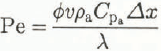
Now, from many runs of the model which included air movement, we observed that the flow rate of the air and imposed temperature difference over the sample control the temperature regime in the sample for a given snow type. The global energy balance is such that the heat carried out by the air flow is primarily balanced by the heat conducted into the sample, with a smaller contribution due to sublimation and condensation within the sample The conduction-advection effects can be characterized by the Peclet number, Pe, which is defined

where υ is a characteristic velocity (the air-flow velocity in the snow), Δx is a characteristic distance (snow sample length) and λ_s is the thermal conductivity of the snow. The higher the Peclet number, the greater the effects of advection of heat due to air flow, relative to the effects of heat conduction. The effects can be seen in Figure 9, which is a non-dimensional plot of temperature versus location, with the Peclet number as a parameter; the input parameters for the profiles illustrated are detailed inTable 3. For all of the cases plotted in the figure, the snow density is 476 kg m⁻³, the thermal conductivity is 0.52 W m⁻¹ K⁻¹, the particle diameter is 1.0 × 10⁻³ m and the mean temperature is −10° C.

Fig. 9. Non-dimensional temperature profiles with Peclet number as a parameter.

Table 3.

It is evident that, for a given imposed overall temperature difference, the greater the air-flow rate, the more curvature has the temperature profile. This means that, the faster the incoming air is moving, the further it can transport its low temperature. A less obvious result is that, for a given flow rate, the greater the temperature difference over the entire sample, the less curvature has the temperature profile. This means that a higher overall temperature difference can better mask the effect of the incoming cold air than can a lower temperature gradient. Thus, circumstances exist where the thermal effects of significant air flow through snow could be neutralized by a steep temperature gradient over the entire snowpack, i.e. there could be significant air movement in the snow that temperature measurements would not reveal, if there is a large temperature gradient over the entire snowpack. These results indicate that the thermal effects of windpumping in natural snow covers are more likely to be observed through temperature measurements when there is a greater flow rate of air in the snow and/or a smaller temperature difference over the entire snowpack than in times of lesser flow rate and steeper temperature difference. Previous investigations in windpumping (e.g. Reference ColbeckColbeck, 1989) have concentrated on the flow rate but have not considered the effect of the overall temperature difference. We will further explore the multi-dimensional thermal effects of windpumping in upcoming laboratory and theoretical investigations.

Conclusions

The thermal regime resulting from forced air flow through a snow sample has been studied numerically. It is demonstrated that the heat transfer associated with vapor transport is significant in the determination of the overall temperature profile but that the major effects are controled by the flow of dry air through the snow and the temperatures imposed at the boundaries. Thus, for applications concerned only with temperature predictions, mathematical calculations need to consider heat advected by the air movement and heat conduction, but may ignore vapor transport. It has been shown that the thermal effects of ventilation of snow are more likely to be observed when there is a greater flow rate of air in the snow and/or a smaller temperature gradient over the entire snowpack than in times of lesser flow rate and higher overall temperature differences. This indicates that there may be occasions when significant air flow through a snowpack exists, but is not detectable by temperature measurements, since the temperature difference over the entire snowpack is high relative to the advected heat. It is also concluded that effective conductivities for ventilated snow have no application for predicting temperatures in ventilated snow.

A new model for calculating vapor transport in snow is presented which allows for the determination of the effects of sublimation. Results of the model show very good agreement with analytical and experimental results. Although in ventilation situations the temperature profiles are controled by conduction and advection, the calculation of vapor transport will be important for mass-transfer considerations. The model holds promise for future developments in sublimation problems in snow-packs, such as ablation of a snowpack or mass redistribution within a snowpack due to temperature gradients.