1. Introduction
Glacier surging is a manifestation of an oscillation in glacier flow which is caused by an internally triggered instability, leading to alternating cycles of slow and fast flow. The increase in ice velocity during a glacier surge, which can be very dramatic, results from the effects of a positive feedback. Reference RobinRobin (1955) was the first to point out that such a positive feedback could be associated with the fact that thicker ice warms the bed, and thus can lead to increased velocities, either through meltwater generation and enhanced sliding1 (Reference ClarkeClarke, 1976) or through the thermal activation of shear flow in the ice (Reference Clarke, Nitsan and PatersonClarke and others, 1977; Reference Yuen and SchubertYuen and Schubert, 1979). In Reference ClarkeClarke’s (1976) description, during slow flow (quiescence) cold ice is immobile and frozen to its bed; during the surge, warm ice “slides”, and the sliding produces frictional heating, further meltwater and thus further sliding. Clearly such a mechanism cannot explain surges of temperate glaciers such as Variegated Glacier, Alaska, U.S.A. (Reference Bindschadler, Harrison, Raymond and GantetBindschadler and others, 1976). This lack of generality has led to some disregard for thermal regulation as a control for glacier surges. Despite this, many authors acknowledge that the thermal regime must influence surging (Reference Clarke and GoodmanClarke and Goodman, 1975; Reference ClarkeClarke, 1976), and indeed the presence of an internal radio-echo sounding reflector (believed to be a surrogate for a polythermal regime) seems to be related to the occurrence of glacier surging in Svalbard (Reference Hamilton and DowdeswellHamilton and Dowdeswell, 1996; Reference Jiskoot, Murray and BoyleJiskoot and others, 2000).
In this paper we present a model for thermally regulated surging of polythermal glaciers overlying extensive soft sediments. We believe that this model might be applicable to glaciers such as Bakaninbreen, Svalbard, and Trapridge Glacier, Yukon Territory, Canada. Both of these glaciers are polythermal and overlie metres thick layers of sediments, which have been shown to be actively deforming. Both glaciers have been extensively studied through borehole and other instrumentation, and these data allow verification of the baseline assumptions of the modelling exercise.
Bakaninbreen
Bakaninbreen (77°45′ N, 17°16′ E) is a 17 km long surge-type glacier situated in southern Spitsbergen, Svalbard. It attains depths of about 300 m, and is 1–2 km wide. The bed slope α is about 0.8° (at least over some of the bed (personal communication from A. Smith, 2000)), so that sin α ≈ 0.014. At about 6.5 km from the glacier front the glacier is confluent with Paulabreen and makes a 90° bend (Fig. 1). Down-glacier from this confluence, the two glaciers flow, separated by a medial moraine, to the head of Van Mijenfjorden. The glacier has been undergoing prolonged retreat, probably of 14.5 km over the past 500–600 years; more recent retreat has averaged 80–100 m a−1 between 1977 and 1990. The glacier overlies bedrock of highly erodible sandstone and friable mudstones (Reference Salvigsen and WinsnesSalvigsen and Winsnes, 1987).

Fig. 1. Propagation of surge front at Bakaninbreen. (a) Front propagation between 1985 and 1986 was associated with a radio-echo sounding internal reflecting horizon, believed to delineate the transition between cold and warm ice, coincident with the geometry and position of the surge front. (b) Propagation of the front throughout the prolonged active surge phase. After Reference Murray, Dowdeswell, Drewry and FrearsonMurray and others (1998).
Bakaninbreen began a prolonged 5–10 year surge in 1985. The surge was characterized by the passage down-glacier of a sharp surge front, approximately 50 m high, travelling at rates of 1.0–1.8 km a−1 (Reference Murray, Dowdeswell, Drewry and FrearsonMurray and others, 1998). The velocity of this front was greater than the ice velocity, which is of the same order (up to 4.5 m d−1) up-glacier from the front, but virtually stagnant below (< 2 m a−1). Down-glacier from the surge front, vertical velocities were positive, measured at up to 0.1 m d−1 (Reference Murray, Dowdeswell, Drewry and FrearsonMurray and others, 1998). Up-glacier from the front, horizontal ice velocities were high, but vertical velocities fell until some 500 m up-glacier from the front vertical velocities became negative and extensive crevassing occurred. Ice and surge-front velocities dropped systematically through the surge, except for a brief speed-up during 1988–89 (Fig. 1). Surge-front propagation is thought to have occurred by a combination of ductile and brittle deformation (Reference Murray, Gooch and StuartMurray and others, 1997, Reference Murray, Dowdeswell, Drewry and Frearson1998).
Thermal regime
The thermal regime of Bakaninbreen is not well known, although there is some suggestive evidence. In Svalbard, glacier thermal regimes seem to be largely controlled by ice thickness. A glacier needs to be thicker than approximately 100 m to be warm-based, whereas ice thinner than about 60 m is typically cold-based. For example, Finster-walderbreen is warm-based where the ice is approximately 120 m thick (Reference Ødegård, Hagen and HamranØdegård and others, 1997); Scott Turnerbreen is cold-based and has a maximum thickness of approximately 55 m (Reference HodgkinsHodgkins, 1997). The ice thickness of Bakaninbreen is such that we should expect the upper portions to be warm-based (>200 m thick; Fig. 1) and the lower portions to be cold-based (<70 m thick close to the margin).
The presence of an internal reflecting horizon (IRH) in radio-echo sounding in 1985 and 1986 (Fig. 1) suggests that the bed was warm up-glacier from the surge front at these times. An IRH is normally interpreted either as the level of the piezometric surface in the glacier or as the interface between cold, upper layers of ice and warm, lower layers (e.g. Reference Hagen and SætrangHagen and Sætrang, 1991; Reference BjörnssonBjörnsson and others, 1996; Reference Ødegård, Hagen and HamranØdegård and others, 1997). At Bakaninbreen, the first interpretation seems unlikely. The IRH occurs at a height above the bed equivalent to 20–26% of the ice thickness, and water pressures would be expected to be much higher than this in order to facilitate fast flow during the active phase of surging. It seems likely, therefore, that this horizon depicts the zero-degree isotherm within the ice (i.e. the transition from cold to warm ice (Reference Ødegård, Hagen and HamranØdegård and others, 1997)). The radio-echo sounding from 1986 shows the IRH mirroring the topography of the surge front and intersecting with the bed close to its base. This is suggestive of a thermal boundary between warm-based surging ice and cold-based non-surging ice very close to the topographic expression of the surge front.
There were no further investigations of the thermal regime until the late phases of the glacier surge. During 1994 four thermistor strings were installed in the glacier. These thermistors show typical 10 m temperatures of −5°C up-glacier of the surge front and −3°C below it where the ice is cold-based (basal temperature −0.17 ± 0.05°C). Furthermore, the apparent viscosity of basal sediments down-glacier of the surge front is sufficiently high to suggest that these sediments are frozen (Reference PorterPorter, 1997). Finally, data from ground-penetrating radar surveys have been interpreted as providing evidence of large ice lenses beneath the glacier bed in the region down-glacier from the surge front (Reference MurrayMurray and others, 2000). Up-glacier of the surge front, the same data are thought to provide evidence of a warm ice layer near the bed which results in increased scattering (Reference Murray, Gooch and StuartMurray and others, 1997, Reference Murray2000).
Thus we suggest that prior to the glacier surge the glacier was warm-based in its upper portions and had cold-based margins and snout. During the active phase of glacier surging, the fast-moving ice was warm-based, whereas ice down-glacier from the front was frozen to the bed. The propagation of the surge front appears to have been associated with the propagation of the warm–cold ice boundary down-glacier (Reference MurrayMurray and others, 2000).
Basal conditions
Only the region of the bed close to the surge front is well known, having been investigated by borehole drilling and sampling of basal sediments. In this region the bed consists of mixed till and marine muds probably greater than 1–3 m in thickness (Reference Hambrey, Dowdeswell, Murray and PorterHambrey and others, 1996; Reference Murray, Gooch and StuartMurray and others, 1997; Reference PorterPorter, 1997; Reference Porter, Murray and DowdeswellPorter and others, 1997). Up-glacier from the current position of the surge front these sediments are actively deforming to a depth of at least 0.4–0.6 m (Reference PorterPorter, 1997) . The inferred viscosity of the sediments varies between 1010 and 1013 Pa s, and their hydraulic conductivity has been measured as 7.7 × 10⁻⁸ −3.2 × 10⁻⁷ m s−1, which corresponds to a permeability of 1.4 × 10⁻¹⁴ −5.8 × 10⁻¹⁴ m2 (Reference Porter and MurrayPorter and Murray, 2001). Beneath the till layer, the bedrock probably has a somewhat lower conductivity of ∼10 m s−1 (Reference Freeze and CherryFreeze and Cherry, 1979), or a permeability of ∼ 1.8 × 10⁻¹⁵ m2.
Hydrology
Bakaninbreen currently terminates at the water’s edge, making any sampling of basal water exiting the margin, either as ground-water or as stream-flow, impossible. However, there is little evidence that surface meltwater reaches the glacier bed at Bakaninbreen: pressure transducers do not show diurnal fluctuation during summer and there are no active moulins at the glacier surface. Englacial drainage appears to be limited to water flow along the planes of faults and shear zones. During the active phase of the glacier surge, surface water presumably entered the glacier through the wide-scale crevassing that occurred up-glacier of the surge front, potentially reaching the glacier bed. More recently, despite extensive hot-water drilling in 1994 and 1995, only 10 holes of 65 that reached the glacier bed connected immediately on completion, and several of these drained through known faults. It is thought that water escapes from warm regions of the glacier bed via groundwater flow or through fractures either at the ice/bed interface or extending to the ice surface.
Trapridge Glacier
Trapridge Glacier (61°14′ N, 140°20′ W) is a 4 km long surge-type glacier situated in the St Elias Mountains, Yukon Territory. A typical thickness is 70 m, and a typical velocity 30 m a−1. The bed slope α is about 7°, so sin α ≈ 0.12. The glacier bed consists of thick sequences of unconsolidated sediments, which overlie a flood basalt, underlain by heavily fractured low-grade metamorphic carbonates (Reference SharpSharp, 1943). The boundary between these rock types is associated with weathering and contact metamorphic clays. Trapridge Glacier last surged around 1941, and by 1949 the glacier had advanced “far beyond its 1941 boundary” (Reference SharpSharp, 1951). The current glacier geometry looks similar to the geometry prior to the 1940s surge. The glacier has been extensively studied since 1969 (Reference Clarke, Collins and ThompsonClarke and others, 1984; Reference Clarke and BlakeClarke and Blake, 1991), resulting in a dataset unrivalled in both longevity and scope.
Thermal regime
Trapridge Glacier is polythermal, with typical 10 m temperatures of −5°C (Reference Jarvis and ClarkeJarvis and Clarke, 1975; Reference Clarke and BlakeClarke and Blake, 1991) . It reaches the melting point only in a central bed area bounded by cold ice. There is not thought to be any thickness of warm ice overlying the region of temperate bed. The warm–cold boundary has been associated with the development and propagation of a 60–70 m high bulge of ice. As the glacier has thickened, the bulge has propagated down-glacier at a rate of approximately 30 m a−1, and the zero-degree boundary has also migrated down-glacier. This migration of the thermal boundary is thought to have occurred at a slower rate than propagation of the geometric feature, but drilling failed to penetrate to the bed due to a thick sediment layer, so measurement of the temperature of basal ice close to the front was prevented (Reference Clarke and BlakeClarke and Blake, 1991).
Basal conditions
Basal conditions are well known in the central warm-based region of Trapridge Glacier: the bed consists of extensive deformable and somewhat permeable glacial till (Reference Clarke, Collins and ThompsonClarke and others, 1984; Reference ClarkeClarke, 1987; Reference BlakeBlake, 1992; Reference Blake, Clarke and GérinBlake and others, 1992; Reference Stone and ClarkeStone and Clarke, 1993; Reference Waddington and ClarkeWaddington and Clarke, 1995). This till has been shown to be actively deforming to a depth of at least 0.3 m beneath the region of temperate basal ice (Reference Blake, Clarke and GérinBlake and others, 1992), has an estimated viscosity of 3 × 10⁹ − 1.8 × 10¹⁰ Pa s (Reference Blake, Clarke and GérinBlake and others, 1992; Reference Fischer and ClarkeFischer and Clarke, 1994) and has a hydraulic conductivity estimated to range from 1.35 × 10⁻⁹ to 3.6 × 10⁻⁷ m s−1, corresponding to permeabilities of 2.5 × 10⁻¹⁶ to 6.5 × 10⁻¹⁴ m2 (Reference StoneStone, 1993; Reference Waddington and ClarkeWaddington and Clarke, 1995). The bedrock underlying the till is probably of a somewhat higher conductivity, around 10 ms (permeability 1.8 × 10⁻¹³ m2) (Reference Freeze and CherryFreeze and Cherry, 1979) because of its fractured nature (Reference SharpSharp, 1943). The upper till layer is considered to consist of two layers, with a low-permeability matrix-rich till underlying a more transmissive cobble-rich unit (Reference StoneStone, 1993).
Hydrology
Water pressure, turbidity and conductivity are routinely monitored beneath the warm-based central region of Trapridge Glacier (e.g. Reference Stone, Clarke and BlakeStone and others, 1993; Reference Stone and ClarkeStone and Clarke, 1996) . During the summer, basal hydrological conditions show diurnal variation, so it is assumed that surface water reaches the glacier bed freely (e.g. Reference Stone and ClarkeStone and Clarke, 1996). Under most conditions this supraglacially derived water together with water from melt of warm basal ice is continuously evacuated from the glacier. Occasionally (less than once a year) short outbursts of basal water lasting a few days appear in the marginal stream, which normally consists of supraglacial runoff only (Reference Stone and ClarkeStone and Clarke, 1996).
Hot-water drilling reveals three types of response on reaching the bed: unconnected holes which do not drain; connected holes at low pressure in which the water level drops; and occasionally, connected holes at high pressure from which artesian outflow occurs.
These observations lead to a conceptual model for the hydrology of Trapridge Glacier (after Reference StoneStone, 1993; Reference Stone and ClarkeStone and Clarke, 1996).
1. Water escapes from the warm region of the glacier bed continuously as ground-water flow passing beneath marginal permafrost and emerging in the forefield as springs. This route drains the majority of basal water spatially and temporally from both connected and unconnected regions. Drainage is probably facilitated by high-permeability regions in the till or “pipes”.
2. Input of surface water and generation of subglacial melt-water creates local “blisters” of water which are hydrologically connected to one another over distances of the order of 10 m; these blisters form the connected water system. Water pressure in these blisters is typically below that in the unconnected system (Reference Murray and ClarkeMurray and Clarke, 1995), so they must be connected to some form of outlet, presumably preferential drainage routes through the basal sediments. Typical flow rates through this system of blisters are 40–50 m h−1 (Reference Stone and ClarkeStone and Clarke, 1996). The areal coverage of blisters drops through closure by ice and sediment creep during periods of low water input (winter).
3. Sudden input of surface water can exceed the capacity of the connected blister system, causing a release event (e.g. Reference StoneStone, 1993; Reference Stone and ClarkeStone and Clarke, 1996). These events are rare and occur less than once per year. Before such events, water pressure in the connected blisters exceeds overburden; this pressure is relieved by opening an evacuation route for basal water through cold marginal ice. For example, a release event on 22 July 1990 resulted in outflow of dyed basal water over 2–3 days (Reference StoneStone, 1993). However, it is difficult to estimate the volume of water involved.
4. The areal coverage of connected blisters at the glacier bed is sufficiently low for them not to affect glacier dynamics significantly. For example, the event of 1990 is not thought to have been associated with a mini-surge (Reference Stone and ClarkeStone and Clarke, 1996), and the effect of temporal variations in water pressure is not detected in surface velocity measurements (Reference Clarke, Meldrum and CollinsClarke and others, 1986).
Thermally controlled surging
We presuppose a till layer beneath a polythermal surging glacier and assume that at the beginning of the surge cycle (at the end of a prior surge) the glacier is cold-based and frozen to its bed, at least in marginal regions and possibly over the entire bed. In the latter case, build-up of ice in the upper part of the glacier becomes sufficient to raise part of the glacier bed to the pressure-melting point. Meltwater from this warm part of the bed is evacuated through the till layer either vertically to underlying high-permeability bedrock or horizontally to the glacier margin beneath marginal permafrost. Increasing basal meltwater production and possibly surface input of water raises pore-water pressures towards flotation pressure, reducing effective pressure and weakening the till. This causes failure of the till, resulting in dilation. The dilated till acts as a reservoir for basal water. Accelerated deformation of the weakened till causes increased basal motion, resulting in an increase in heat production and thus creating further meltwater at the bed. This meltwater in turn raises pore-water pressure further. This positive feedback is the suggested surge mechanism.
Storage in the pore space of dilated till and evacuation through ground-water flow may be sufficient to cope with all of the meltwater produced at the bed, particularly if the hydraulic conductivity of the bed material is high. We might suppose (correctly, as it turns out) that a stable ice flow could then occur, where the negative feedback associated with high transmissivity is able to compensate for the positive feedback due to the ice-flow/meltwater generation loop. However, if the hydraulic conductivity of the bed is low, we expect there to be ponding of water in “blisters” at the ice/bed interface. The build-up of water pressure in these blisters will result in release of water at the ice/till interface, such as the events seen at Trapridge Glacier, or through the surface of the glacier (e.g. through faults at Bakaninbreen; cf. Reference Skidmore and SharpSkidmore and Sharp, 1999). If we suppose that the areal blister fraction is similar to the fraction of boreholes which “connect” to the water system, in other words is relatively small, then the stiffness of most of the till is controlled by the pore-water pressure, rather than the blister pressure, and it is this which therefore controls resistance offered to the ice flow by till deformation. We might suppose that this pore pressure is unrelated to the blister pressure, which presumably will respond over short time-scales to surface meltwater input.
In our model, we will begin by ignoring discharge associated with blister events, and will also assume that all the resistance to the flow is associated with deformation of the till. We will find, however, that neither of these assumptions is viable, and in particular, it is crucial in the model to account for the blister discharge events.
The rest of the paper is organized as follows. In section 2 we construct a mathematical model which represents, in the simplest way possible, the interacting components of ice flow, meltwater evacuation and till deformation. As we have found in previous surge theories (Reference FowlerFowler, 1987; Reference Fowler and JohnsonFowler and Johnson, 1995), it is extremely useful to construct from this a zero-dimensional model, and this is done in section 3, where the model is reduced in this way to two ordinary differential equations for the ice thickness and the basal effective pressure. These equations have a unique steady state (generally), which is stable for high subglacial transmissivity, but oscillatorily unstable for low transmissivity. If the transmissivity is very low, then the effective pressure decreases towards zero, and it is in this case that surge-like behaviour can occur. The violence of the surge is associated with the form drag offered by the bed, and the efficiency of the blister discharges. Section 4 offers some conclusions for the interpretation of the behaviour of Trapridge Glacier and Bakaninbreen in the light of these model results.
2. Mathematical Model
We propose a model (see Table 1 for nomenclature) which accounts for the longitudinal variation of ice depth and velocity with downstream position x, and we ignore three-dimensional effects associated with transverse flow variation and also with vertical variation of, for example, ice velocity or temperature gradient, preferring to parameterize these latter effects in a suitably realistic way.
Table 1. Nomenclature

The basic equation is that of mass conservation,
where h is the ice depth, u is the (mean) downstream velocity, A is the accumulation/ablation rate, and subscripts denote partial derivatives with respect to time t or downstream distance x. The geometry we have in mind is shown in Figure 2.

Fig. 2. The thermal geometry of the model. The frost-line rises to the ice/till interface underneath the glacier, and subglacial meltwater flows as ground-water to an outlet spring lower down.
The ice velocity is essentially supposed to be due to basal motion caused by the deformation of a water-saturated layer of till, of thickness h s, at the base. It is also properly necessary to allow for a small component of shearing in the ice. We define the “sliding” velocity to be u s and the (averaged) shear deformation velocity to be u d, so that
and we might then prescribe

where τ is the basal shear stress, and η i is a depth-averaged ice viscosity, appropriately defined to reflect the averaged nature of u d. The shear stress takes the usual ρ i gh sin α form, where ρ i is ice density, g is gravity and sin α is the down-flow slope, together with corrections reflecting variations in surface slope and longitudinal stress (Reference FowlerFowler, 1987), each of which, though small, provides diffusive terms which may be expected to be important in describing propagating surge fronts (Reference FowlerFowler, 1989):
Here η i is the vicosity of ice, taken as constant.
The “sliding” (or “basal-motion”) law takes a form popularized by Reference Boulton and HindmarshBoulton and Hindmarsh (1987),
![]() , where N is the effective (overburden minus pore-water) pressure, and p and q are dimensionless exponents with typical values less than one. This law has the advantage of simplicity (u
0s increases with τ and decreases with N) but the disadvantage of little, if any, experimental veracity. Work by Kamb and co-workers (Reference KambKamb, 1991; Reference Engelhardt and KambEngelhardt and Kamb, 1998) and field data (Reference Hooke, Hanson, Iverson, Jansson and FischerHooke and others, 1997) strongly suggest a visco-plastic law in which motion occurs at a yield stress τ
f, and we would expect such a Coulomb friction-derived flow law to have τ
f = μN, where μ is a coefficient of friction. As pointed out by Reference BoultonBoulton (1996), such a plastic law is included in the Boulton–Hindmarsh law through the limits p → 0, q → 1. We do not wish to become embroiled here in a debate about till rheology; what we have to say is not fundamentally based on the choice of a viscous rheology.
, where N is the effective (overburden minus pore-water) pressure, and p and q are dimensionless exponents with typical values less than one. This law has the advantage of simplicity (u
0s increases with τ and decreases with N) but the disadvantage of little, if any, experimental veracity. Work by Kamb and co-workers (Reference KambKamb, 1991; Reference Engelhardt and KambEngelhardt and Kamb, 1998) and field data (Reference Hooke, Hanson, Iverson, Jansson and FischerHooke and others, 1997) strongly suggest a visco-plastic law in which motion occurs at a yield stress τ
f, and we would expect such a Coulomb friction-derived flow law to have τ
f = μN, where μ is a coefficient of friction. As pointed out by Reference BoultonBoulton (1996), such a plastic law is included in the Boulton–Hindmarsh law through the limits p → 0, q → 1. We do not wish to become embroiled here in a debate about till rheology; what we have to say is not fundamentally based on the choice of a viscous rheology.
We make two modifications to the Boulton–Hindmarsh sliding law. One reflects the situation (which we refer to as a sub-temperate base) where the till is only partially melted (Fig. 3). In this case, the unfrozen till has a thickness s < h s, and it is only this part of the layer which deforms. The second modification is to allow the inclusion of what we term vestigial stress, which arises from the viscous ice flow over the undulating till layer. The reason for its inclusion is as follows. The Boulton–Hindmarsh law implies an infinite velocity at zero effective pressure. We suppose that N is determined by a consolidation relation of the form
where w is the pore-water volume fraction of the saturated till. The typical form of such consolidation laws is shown in Figure 4 (Reference HillelHillel, 1980), and in particular N reaches zero at a finite value of w, namely, w m (w m may be thought of as the value of the moisture content at which disaggregation of the particulate occurs; for a granular medium it is in the region of 0.4–0.5, but it may be higher for clayey till). In our model, w changes by virtue of meltwater produced by geothermal and frictional melting at the glacier sole, and there is no physical restriction to prevent N reaching zero. Indeed, on a smooth bed, there would therefore be nothing to prevent indefinite acceleration. However, bed undulations will lead to the classical Reference WeertmanWeertman (1957) sliding resistance. This acts additively (Reference FowlerFowler, 1981), so an appropriate sliding law is

where n is the exponent in Glen’s law, and R and R v are roughness coefficients associated, respectively, with till deformation and bed undulation. An additional reason for proposing this additive viscous stress lies in the notion that smooth till beds will spontaneously form undulations through an erosional instability (which, in ice sheets, may form drumlins) (Reference HindmarshHindmarsh, 1998), thus providing an effective roughness even where the underlying topography is very smooth. It may be the case that this viscous stickiness dominates in ice streams, for example, but in the present paper we will assume it has a relatively small effect.

Fig. 3: The three thermal regimes at the bed: warm, sub-temperate and cold.

Fig. 4. The typical form of the suction characteristic curve. w m is the value where disaggregation of the solid grains would occur.
Where the till is wet, we suppose that there is some method for the evacuation of the meltwater. If we suppose the substrate is permeable, then a simple representation for the evacuated meltwater flux U is

where ρ i gh − N is the pore-water pressure in the till, so that if h b and l d are the vertical and horizontal distances downstream to the mouth of the outlet drainage channel, (ρ i gh − N + ρ w gh b)/l d is the hydraulic gradient; k p is the substrate permeability, η w is the viscosity of water, and ρ w is the density of water. Thus Equation (2.7) is a simple representation of Darcy’s law which avoids the complexity of solving a two- or three-dimensional ground-water flow model.
The permeability k p here represents the permeability k sub of the substrate, estimated by Reference Clarke, Collins and ThompsonClarke and others (1984) as ∼10−13 m2 . If the till is much less permeable, with permeability k till, then downstream percolation through the till can be neglected, and an appropriate effective permeability is obtained by supposing water flow occurs through till and substrate in series, whence

So far, we have seven Equations (2.1–2.7) for the eight variables h, u, u s, u d , τ, N, w and U. The final equation determines the moisture content w of the till or, where the base is frozen, the depth of the permafrost boundary. We define a heat-budget velocity

where G is the geothermal heat flux, ρ w is the density of water and L is the latent heat, so that f is a velocity; q i is the heat flux into the (cold) ice above the base, and we assume a simple conductive cooling law
although more ambitious parameterizations can (and in later work will) be made; k T is the thermal conductivity, and ΔT is the temperature drop between base and surface, essentially the sub-cooling at the surface, and taken as fixed.
We now distinguish three possible basal thermal regimes.
1. Cold (C)
The base is frozen, and the thermodynamic variable is the depth of the freezing front Σ (Fig. 3). If ψ is the porosity of the substrate, then the Stefan condition for the evolution of Σ is
assuming a large aspect ratio so that Σ varies slowly with x. Note that u s = 0, and also s = 0, which is consistent with the sliding law (Equation (2.6)). To be strict, q i in Equation (2.10) should be kΔT/(h + Σ) if Σ > 0, but the effect is minor. Equation (2.11) applies so long as Σ > 0, and when Σ reaches zero, we switch to region S.
2. Sub-temperate (S)
In this region, the till is partially melted to a height s above the till/substrate interface, and contains a water volume fraction w. We expect the downstream water flux through the till to be negligible, so conservation of water mass in the till implies
in addition, energy conservation (the Stefan condition) at the freezing interface implies

where ϕ(z, x, t) is the porosity of the frozen till at height z above the bed (z > s). The second condition applies if freezing is occurring, i.e. ∂s/∂t < 0; then it is the water fraction w (implicitly assumed uniform through the till, which means that gravity-induced gradients in N are neglected) which is frozen in at s. On the other hand, when melting is occurring (f > 0), it is the previously frozen ice fraction (as water equivalent) ϕ|s which melts: ϕ may vary with s, since w will generally vary with time. Specifically, we specify ϕ(z, x, t) for s < z < h s by the relation
and we also specify the initial value of ϕ at t = 0 where s > 0.
If s reaches zero, we revert to the cold base (C); if s reaches h s, we reach conditions for a warm base (W).
3. Warm (W)
The base is warm when the till is unfrozen but the ice above the ice/till interface is below the freezing point; in this case, s = h s and mass conservation of water implies
We enter region W from S when f > 0 (melting). If f becomes negative we return to S and freezing is initiated.
Most generally, we should also include a fourth part of the base, temperate (T), where the ice above becomes temperate. This will occur if viscous heating in the ice is too strong for the conductive cooling. This appears to be the case at Bakaninbreen, as noted. This effect is, however, neglected in this model.
If ∂s/∂t < 0 in the sub-temperate region S, then the saturated till is being frozen. In this situation, frost heave can occur, and discrete ice lenses could occur. We ignore such possibilities because the lenses are often very thin, and their separate existence does not practically affect the theory. However, frost-heave theory indicates that lens formation can terminate, leading to the formation of a final massive lens, and it has been suggested that the formation of this massive lens is the cause of massive ground ice in the Canadian Arctic (Reference Fowler, Noon and KnutssonFowler and Noon, 1997) . Indeed it may also be a mechanism for entrainment of basal debris into glaciers and ice sheets. But the theory suggests that massive lens formation will take place on very long time-scales, so we neglect the possibility here.
3. A Lumped Parameter Model
We will limit our attention in this paper to the study of a simplified form of the model presented above, which is a “lumped” model in the terminology of Reference Fowler and SchiaviFowler and Schiavi (1998), insofar as it retains the essential physical processes while ignoring details, and specifically, spatial variation. One can think of obtaining this lumped model by integrating the model over the length of the glacier. In a sense, the model is already lumped through simplified prescriptions for U and q i, for example. While we had hoped in the present paper to also include solutions of the spatially varying model, extensive investigations show that it is not entirely trivial to obtain such solutions, and their presentation will be deferred to future work. Partly, the difficulty lies in the fact that extra physical mechanisms must be introduced, notably in dealing with the propagation downstream of a sub-temperate/cold transition point.
In the lumped model, conservation of ice mass is expressed as
where l is the glacier length and B is the mass balance (more specifically, we can interpret B as the yearly balance integrated over the accumulation area). The overdot denotes a derivative with respect to time. For simplicity, we choose to ignore the shear deformational velocity u d, and also the diffusive stress effects. These terms are likely to be important in the spatially varying model, however. Thus
and the sliding law for warm-based ice is
We suppose a consolidation law of the form
and that the water content satisfies
with the efflux being just
and the heat-budget velocity is

We ignore separate cold or sub-temperate regions. It is possible to modify the definition of w(N) to allow for w < 0 indicating freezing, but it will turn out that our problems are more associated with N reaching zero.
Equations (3.1) and (3.5) give two ordinary differential equations for N and h, with the subsidiary variables τ, u, w, f and U being given by Equations (3.2), (3.3), (3.4), (3.6) and (3.7). We choose scales [h], [u], etc., for the variables h, u, etc., by choosing balances in the equations as follows:

where w m is the maximum water saturation, and w′(N) = dw/dN is the derivative of w as a function of N. (If this is variable, then we should use a typical value instead.) To get useful estimates, it is better in practice to use observed values of [u] and [h] to infer sensible values of the somewhat heuristic parameters B and R.
We then write h = [h]h*, etc. The resulting dimensionless equations for N* and h* are, omitting the asterisks henceforth,

where
and the parameters are

In supposing that δ is a constant, we are really assuming that N depends linearly on w, and specifically that N = [N][1 − (w/w m)]. In reality, δ should be a decreasing function of N (Reference ClarkeClarke, 1987). We use values

and from these we infer

Using Equations (3.12) and (Reference Clarke, Collins and Thompson3.13), we find typical values of the parameters as follows:

and we use these as guides. For a wavy bed, we could expect ε ∼ 1, but if the undulations are smooth, then ε ≪ 1. We shall assume ε is non-zero but small, and consider its effect only when it is necessary (when N ≈ 0).
Note that the parameter β is proportional to the permeability k p Reference Freeze and CherryFreeze and Cherry (1979) quote ranges 10−13 − 10−19 m2 for subglacial till, while their range for fractured rock is 10−11− 10−15 m2. Evidently, effective values of k p given by Equation (2.8) may vary widely, so that values of β may be large or small; β thus stands out as the most obvious behavioural bifurcation parameter. As we shall see, the other crucial parameter is δ. In this context, our comments above on its variability with N require some consideration.
The simple model (Equation (3.9)) which we have derived for h and N implicitly assumes that the basal till is warm, whereas we should in reality allow for freezing to occur. Simplistically, Equation (2.11) can be used to extend the applicability of Equation (3.5) to negative values of w if we interpret these as representing depth of the frost-line below the glacier. In terms of N, with constant δ and dimensionless N = 1 when w = 0, freezing then corresponds to N > 1, and the only modification we need to make to the lumped model is to force u = U = 0 when N > 1. This is easily, if artificially, done, and we make some comments on the effect on numerical results below.
It is less easy to cater for a more realistic consolidation law in the simple lumped model, since for laws in which N → ∞ as w → 0, we would have δ → 0 as N → ∞, but no switch to a frozen base can occur unless we include the sub-temperate description (2.12), and we resist this until we treat the spatially varying case. We do, however, recognize that effective values of δ may be substantially lower than that given in Equation (3.14).
Analysis of the lumped model
Eliminating the algebraic variables and putting ε = 0 for the moment, we have

where
If p = q = 1/2, then c = 3 and b = 1, whereas the Coulomb plastic law where p = 0, q = 1 would be obtained if c = 1 + b, and c → ∞. We aim to construct the phase portrait of the solutions in the (h, N) plane. The h nullcline (where
![]() ) is N = hc
/b
(Fig. 5). The N nullcline (i.e. where
) is N = hc
/b
(Fig. 5). The N nullcline (i.e. where
![]() ) is given by the solution of
) is given by the solution of

Fig. 5. The nullclines
![]() and
and
![]() of Equations (3.15). The values used are β = 0.1, v = 0.5, c = 3, b = 1, and γ = 0.15. The arrows on the diagram reflect the direction of evolution of N if δ is small; the upper branch of the N nullcline is stable, but as h increases on it, there is a crisis at the nose, when the trajectory falls off it and N decreases abruptly.
of Equations (3.15). The values used are β = 0.1, v = 0.5, c = 3, b = 1, and γ = 0.15. The arrows on the diagram reflect the direction of evolution of N if δ is small; the upper branch of the N nullcline is stable, but as h increases on it, there is a crisis at the nose, when the trajectory falls off it and N decreases abruptly.
Denote the lefthand side of this equation by L, and the righthand side by R R is a convex function of h, with a minimum at h = (λ/β)1/2. For fixed h, L is a convex function of N. Therefore for a fixed value of h, there are generally two values of N. In particular, two branches exist for small h and these have N ∼ 1/βvh, N ∼ h (c+1)/b as h → 0 (Fig. 5).
It is possible that there could be another branch of the N nullcline, since R is convex. Further study of Equation (3.17) indicates that this is unlikely for the present parameter values, and in any case it does not interfere with our analysis below. We thus suppose the nullclines are as shown in Figure 5.
Writing
![]() ,
,
![]() , the stability of the (unique) fixed point where the nullclines intersect is determined by the trace and determinant of the community matrix
, the stability of the (unique) fixed point where the nullclines intersect is determined by the trace and determinant of the community matrix

evaluated at the fixed point (e.g. Reference MurrayMurray, 1993). It is straightforward to show that the fixed point is stable if it lies on the upper branch of the N nullcline, which is if ∂F 2/∂N = (b/N − βv)/δ < 0. Also (at the fixed point)

and the conditions for a Hopf bifurcation (and thus the generation of a limit cycle) are that
On the lower branch, the slope of the N nullcline is positive and greater than that of the h nullcline, and it follows from this that det M > 0; hence instability occurs precisely if tr M > 0. Since tr M = ∂F 2/∂N − c/h, this condition automatically implies (since then ∂F 2/∂N > 0) that the steady state is on the lower branch. The condition for instability can be written
Roughly speaking, instability occurs if β and δ are low enough; in particular, when β is small, then h ≈ λ/(1 + γ) at the fixed point, and Equation (3.21) is approximately

and for small β, this in turn is approximated by

where δc is defined by this equation. For the values in Equation (3.14), δc ≈ 2.9; if instead λ = 1 (as in some numerical illustrations below), δc ≈ 0.44. These conclusions are qualitatively unaltered in the plastic limit of the Boulton–Hindmarsh flow law, where p = 0, q = 1, so that c/b = 1 and δc = 1.
Now suppose that β and δ are both small. As a function of N,
![]() has negative slope on the upper branch, which is therefore quasi-stable, and thus for δ ≪ 1, N rapidly approaches the upper branch as shown in Figure 5. It then follows this branch down as h increases until it reaches the nose; at this point, N decreases rapidly, and with the model (3.15), N reaches zero in finite time and the model breaks down.
has negative slope on the upper branch, which is therefore quasi-stable, and thus for δ ≪ 1, N rapidly approaches the upper branch as shown in Figure 5. It then follows this branch down as h increases until it reaches the nose; at this point, N decreases rapidly, and with the model (3.15), N reaches zero in finite time and the model breaks down.
We therefore have to consider what happens when N reaches zero. The inclusion of non-zero ε in the sliding law

allows u → (h/ε) n as N → 0, the effect of which on the N nullcline
is to depress it, so that it would intersect the h axis at h ≈ λ 1/(n+2) εn /(n+2). This does not affect the breakdown of the model as N → 0, however.
We have already discussed what we believe can and does happen if N reaches zero. Ponding occurs at the ice/till interface, and these “blisters” grow until at some critical excess pressure a fracture-like event enables the blisters to become connected and discharged. Such a discharge might occur at the snout, or as a blow-out through faults in the glacier. In any event, the existence of such discharges suggests that an additional term to represent blister discharge should be added to the model. There are various ways we might choose to do this. If we retain the second equation in (3.15) as it is, we cannot allow N < 0, and this can be effected by prescribing a dimensionless blister flux C/Nr , where C is a small dimensionless coefficient, and r is a suitable exponent. In addition, it is numerically convenient, and essentially equivalent for N ≥ 0, to represent Equation (3.24) as

where we should choose

to be consistent with Equation (3.24) at N = 0, but will generally take it as constant. The modification of Equation (3.15) 2 which we propose is thus

What is the effect of this on the phase portrait? Nothing is altered for N = O(1), but for small N it is clear that
![]() , so that the N nullcline must be bent round. The resulting nullcline is shown in Figure 6. More complicated situations can occur, but this is the simplest.
, so that the N nullcline must be bent round. The resulting nullcline is shown in Figure 6. More complicated situations can occur, but this is the simplest.

Fig. 6. Nullclines of Equation (3.28). Parameters as for Figure 5, and also
![]() , C = 0.1, f = 0.1. When δ is small, a relaxation oscillation will occur as shown. Note the logarithmic scale for N.
, C = 0.1, f = 0.1. When δ is small, a relaxation oscillation will occur as shown. Note the logarithmic scale for N.
The resulting oscillation when δ ≪ 1 is also illustrated in Figure 6. The quiescent phase is when N is on the upper branch, and u = O(1). On the lower branch, N is low, and blister discharge occurs; u will be large if the form drag (ε) is small, though this is not essential; and the surge terminates when h decreases below a critical value. Finally we note that the suddenness of the surge is associated with the relaxation parameter δ. Recalling Equation (3.11), δ is given explicitly as

The value of δ depends primarily on till thickness. Avalue of h s = 5 m together with [τ] = 0.9 bar gives δ = 0.7. A 1 m thick layer gives a smaller value of 0.14, but one might expect that the vestigial resistance term would be more important in this case. In general, this suggests that even if the motion is oscillatory, it is unlikely to be relaxational.
Numerical results
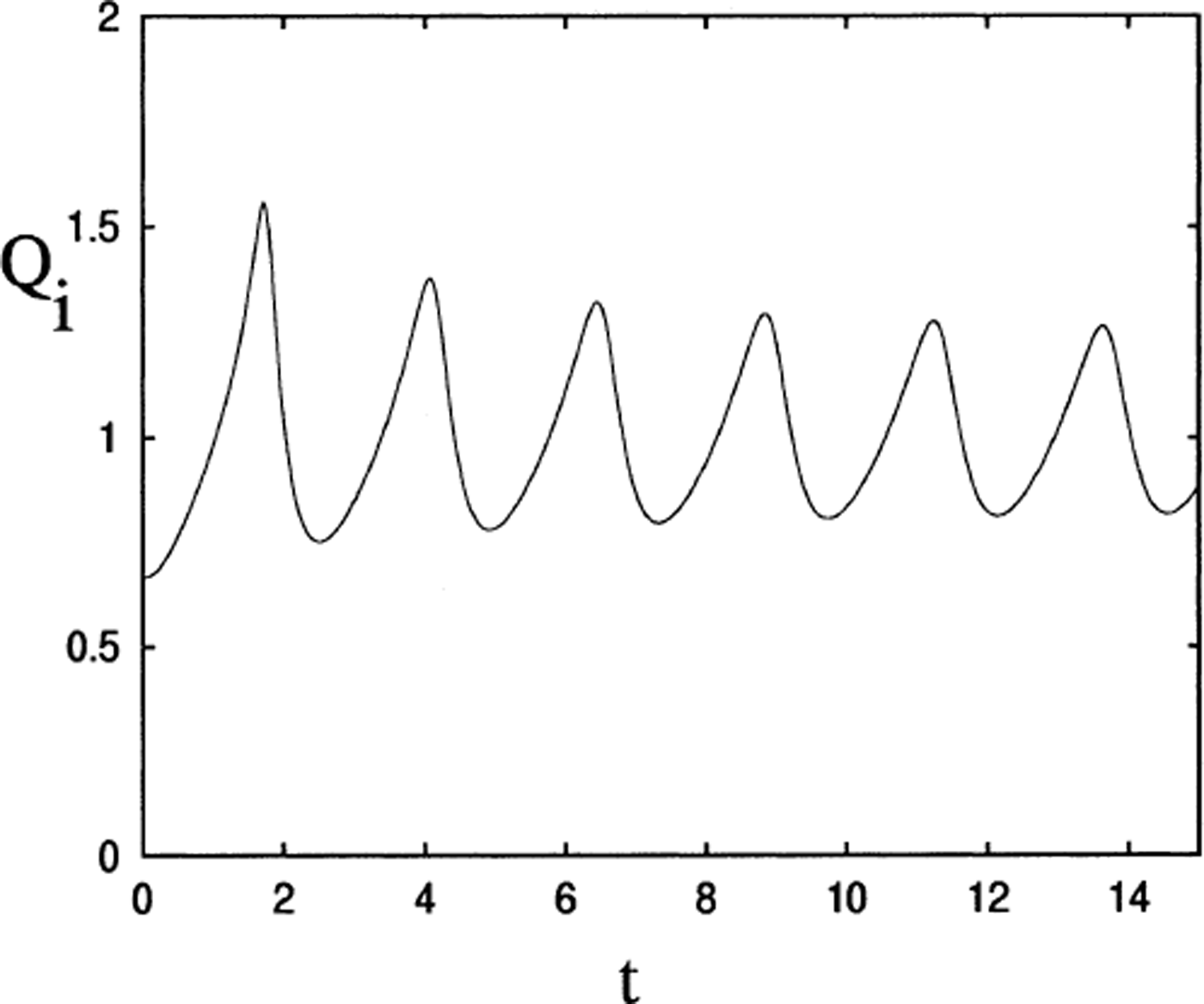
It is straightforward to integrate Equations (3.28), although awkward if C is too small. Figures 7–10 show, respectively, the phase portrait of N vs h, and time series of ice flux Q
i = uh, effective pressure and ice thickness. Note that the variables portrayed are in dimensionless, scaled form. The figures confirm that the lumped model will oscillate if β and δ are small enough. Numerical solution with the same parameters, except that β = 0.5, gives a stable steady state. As discussed above, the dimensionless parameter β, a measure of substrate permeability, is critical in determining whether oscillations occur or not. If β (in this model) is less than a critical value of about 0.315 (other parameters being as in Figure 7), then oscillations occur; and with relatively low values of δ and
![]() , these appear generally to have the form shown in Figure 8, with a rapid surge occurring when the effective pressure reaches zero. However, if
, these appear generally to have the form shown in Figure 8, with a rapid surge occurring when the effective pressure reaches zero. However, if
![]() is larger, oscillations will occur, but without the violent surge. Figure 11 shows an example of this.
is larger, oscillations will occur, but without the violent surge. Figure 11 shows an example of this.

Fig. 7. Phase portrait of N vs h for values of β = 0.1, δ = 0.2, with the remaining parameters being c = 3, b = 1,
![]() , v = 0.5, γ = 0.15, C = 0.1, and r = 1. Note the logarithmic scale for N.
, v = 0.5, γ = 0.15, C = 0.1, and r = 1. Note the logarithmic scale for N.

Fig. 8. Ice flux vs time. Same parameters as Figure 7.

Fig. 9. Effective pressure vs time. Same parameters as Figure 7.

Fig. 10. Ice thickness vs time. Same parameters as Figure 7.

4. Conclusions
We have constructed a simple model to represent the thermal control on the dynamics of a glacier “sliding” (see footnote in introduction) on a layer of deformable till at its base. The model embodies a representation of an idea essentially due to Reference RobinRobin (1955) and subsequently elaborated by Reference ClarkeClarke (1976): increasing thickness of a glacier causes warming at the bed, increased water production and thus enhanced sliding. This positive feedback can lead to surging behaviour, represented here by the instability of the steady state and the existence of periodic flow behaviour. The cyclicity is due to the recovery which occurs following drawdown of the ice.
In our simple model, there are two critical dimension-less parameters which determine instability, denoted by δ and β. Of these, δ is a dimensionless measure of till thickness, while β is a dimensionless measure of effective substrate permeability. Estimates of these parameters, using values of basal shear stress (1 bar), length (10 km), velocity (100 m a−1) and slope (sin α = 0.1) which are typical of Trapridge Glacier, Bakaninbreen and many other glaciers, are found to be of O(1) for values of till thickness 5 m and substrate permeability 10−14 m2. In this simple model, instability and consequent periodic behaviour occurs if both δ and β are sufficiently small, precise criteria being variously Equation (3.21), (3.22) or (3.23). We infer that the current model provides a realistic mechanism for oscillatory surging behaviour of both these glaciers.
Reference Meier and PostMeier and Post (1969) pointed out that surging glaciers come in all shapes and sizes, and that surging covers a range of behaviours. However, there is a common perception that surging should generally be a violent and thus also relatively short-lived phenomenon; Variegated Glacier is perhaps the archetypal example of this (Reference KambKamb and others, 1985), and the expectation of similar behaviour in the surge-type Trapridge Glacier has led to the notion that the advancing front is the precursor to surging behaviour.
pt› We want to suggest a different interpretation here. First we must consider how we expect a spatially dependent version of our current model to behave. We had hoped to include numerical solutions of the spatial model here, but that turns out to be more complicated than one might have expected, and is deferred to future work. However, Reference FowlerFowler (1987, Reference Fowler1989) has solved this problem in a related model, and we can use his results to make an informed guess as to the spatially dependent behaviour. There are two critical parameters which govern the behaviour of the surge (assuming that β is small enough). In the present model these may be taken to be δ and
![]() . (The corresponding roles are taken by ε and δ in Reference FowlerFowler (1989).) The parameter δ represents the thermal transition time, and it determines how fast surge activation occurs. Specifically, when h reaches the righthand nose of the N nullcline in Figure 6 (on the cold, slow branch), we expect that in the spatially dependent model, activation waves will propagate up- and down-glacier, transferring the ice in the central reservoir area to the fast (lower) branch of Figure 6. These activation waves have been observed (e.g. Reference BjornssonBjornsson, 1998). In a temperate glacier, the parameter corresponding to δ represents the transition time between drainage states (channelized or distributed) and is very small, so that activation occurs before any significant ice motion can occur (Reference RaymondRaymond, 1987). This is followed by the surging slump forward of the fast-moving ice; the speed of the ice is controlled by the second parameter, which in our model is the vestigial roughness
. (The corresponding roles are taken by ε and δ in Reference FowlerFowler (1989).) The parameter δ represents the thermal transition time, and it determines how fast surge activation occurs. Specifically, when h reaches the righthand nose of the N nullcline in Figure 6 (on the cold, slow branch), we expect that in the spatially dependent model, activation waves will propagate up- and down-glacier, transferring the ice in the central reservoir area to the fast (lower) branch of Figure 6. These activation waves have been observed (e.g. Reference BjornssonBjornsson, 1998). In a temperate glacier, the parameter corresponding to δ represents the transition time between drainage states (channelized or distributed) and is very small, so that activation occurs before any significant ice motion can occur (Reference RaymondRaymond, 1987). This is followed by the surging slump forward of the fast-moving ice; the speed of the ice is controlled by the second parameter, which in our model is the vestigial roughness
![]() . If
. If
![]() , then the surge is rapid and consequently short-lived.
, then the surge is rapid and consequently short-lived.
It is important to realize that oscillations do not rely on the value of these two parameters being small, so that surging (oscillatory) behaviour is not required to be relaxational in character. The parameters δ and
![]() of the current model and their equivalents ε and δ in Reference FowlerFowler’s (1989) temperate surge model also carry different physical interpretations, although they have equivalent mathematical effects. In a temperate glacier model, the resistance to ice flow is due to bed roughness. In surge conditions at elevated water pressure, this resistance is reduced through the effects of subglacial cavitation. In the present model of thermally controlled surging, however, the primary resistance is provided by till stiffness. At the high water pressures which occur in the surge state, this till stiffness effectively disappears, and the bed roughness provides the vestigial resistance which limits ice velocity. There is nothing which requires this to be small, however.
of the current model and their equivalents ε and δ in Reference FowlerFowler’s (1989) temperate surge model also carry different physical interpretations, although they have equivalent mathematical effects. In a temperate glacier model, the resistance to ice flow is due to bed roughness. In surge conditions at elevated water pressure, this resistance is reduced through the effects of subglacial cavitation. In the present model of thermally controlled surging, however, the primary resistance is provided by till stiffness. At the high water pressures which occur in the surge state, this till stiffness effectively disappears, and the bed roughness provides the vestigial resistance which limits ice velocity. There is nothing which requires this to be small, however.
A comment on this vestigial roughness should be made here. In our (two-dimensional) model, bed roughness was introduced to provide resistance at elevated water pressures. In certain geometries however, this roughness may be more realistically provided by the side-walls. A case in point is Variegated Glacier, where the onset of transition (to high velocities) when the central effective pressure becomes low is postponed because of the higher levels (due to ice buoyancy) of the effective pressure at the bed away from the central drainage artery. The reduction in basal shear stress is supported by an increased lateral shear stress supported at the side-walls, and, in the case of Variegated Glacier, transition is finally associated with a lateral shear rupture of the flow at the walls. A related occurrence is at the margins of the rapid Siple Coast ice streams. We feel that the assumption of two-dimensionality may be less critical for a glacier such as Trapridge, whose aspect is more like that of a (locally) two-dimensional flow.
The activation time-scale parameter δ represents thermal transition in the subpolar case, but drainage transition time in the temperate case. A principal difference between the thermally controlled model and the hydraulically controlled model would seem to be that this parameter will generally be of O(1) in the thermal case.
What then is the consequence of the slower thermal control? Suppose that δ ∼ O(1) (as we infer) but that the bed is vestigially smooth
![]() . Then the thermal activation waves propagate up- and down-glacier relatively slowly (as we see on Trapridge Glacier and Bakaninbreen), but behind the advancing thermal front the activated ice wants to move very fast. However, it is unable to do so, as this would require very fast advance of the surge front, which is prevented by the thermal control. Consequently, the ice behind rapidly flattens out, allaying its propensity for rapid velocities by reducing the basal shear stress. (We have seen this behaviour in some simulations of the spatial model.) Only if the front reaches the glacier snout, and the forefield is warm, will a rapid acceleration then occur.
. Then the thermal activation waves propagate up- and down-glacier relatively slowly (as we see on Trapridge Glacier and Bakaninbreen), but behind the advancing thermal front the activated ice wants to move very fast. However, it is unable to do so, as this would require very fast advance of the surge front, which is prevented by the thermal control. Consequently, the ice behind rapidly flattens out, allaying its propensity for rapid velocities by reducing the basal shear stress. (We have seen this behaviour in some simulations of the spatial model.) Only if the front reaches the glacier snout, and the forefield is warm, will a rapid acceleration then occur.
We think that the front propagation on both Trapridge Glacier and Bakaninbreen is thermally controlled in this way, but we also think that the vestigial roughness is not small, because the long profiles of these glaciers did not flatten out in the way described above. Therefore we infer that the sliding velocities attained on the warm branch of Figure 6 are not large, and therefore that no rapid acceleration will occur. The thermal activation front is also the surge front.
Suppose now that the activation wave speed (controlled by δ) is of similar magnitude to (but less than) the ice velocity on the fast branch. As the activation waves spread out, the ice behind the forward wave develops a growing front. After the thermal wave reaches the snout, the front continues to move forward as a shock wave, and no terminal acceleration occurs. This behaviour appears to be consistent with the recent behaviour of Trapridge Glacier. On Bakaninbreen, the front simply stopped short of the terminus; such behaviour cannot be portrayed within the confines of our model.
We summarize as follows: in thermally controlled surges, activation waves due to warming of the bed spread up- and down-glacier, with the forward front causing an advancing wall of ice to propagate down-glacier (if the surging ice speed is greater than the activation wave speed). This behaviour is what we see onTrapridge Glacier and Bakaninbreen, and is to be interpreted in the present framework as indicating that the value of δ is not small; this indication is consistent with the model (since our estimated typical value of δ is 0.7; see Equation (3.14)). The propagation of the fronts on Trapridge Glacier and Bakaninbreen is an integral constituent of the oscillation which is a glacier surge.
Figures 8 and 11 show two forms of the oscillatory ice flux which can occur in our model, one gentle and the other violent. It is not possible to state precisely from historical evidence which of these two might more closely correspond to the behaviour of Trapridge Glacier. The glacier surged some time between 1941 and 1951, since a photograph by R. P. Sharp on 7 July 1941 and Canadian Government photograph A13136–44 of 9 July 1951 (see Reference Clarke, Collins and ThompsonClarke and others, 1984, fig. 3a) indicate an advance of about 1000 m in the intervening 10 years, apparently due to the advance of the central one of three prominent lobes which are apparent in the 1941 photograph, and also in a 1996 photo by G. K. C. Clarke. This represents a threefold increase in average mean speed over the current front-advance rate of 30 m a−1. Based on the theoretical framework of the present paper, we would surmise that a repeat of the 1941 surge would take the form of a gradually accelerating front, with the crevassed state indicated in the 1951 photograph perhaps indicating that Figure 8 is more relevant, and an identifiable rapid last “surge” may occur. Our main thesis is that the current slow front propagation is an essential part of this process.
Acknowledgements
We are grateful for information and comments from A. Hubbard, who provided copies of Trapridge photographs of 1941 and 1996. We thank U. H. Fischer for his comments on the behaviour of Trapridge Glacier, and R. Le B. Hooke for his diligence as Scientific Editor.