


List of Symbols

1. Introduction
The increase in the offshore drilling operations which has taken place in the last decade in the Arctic Ocean has placed demands for a more detailed sea-ice prediction model.
Presently, the methods applied for the prediction of sea ice fall within three main categories: the thermodynamic approach, the statistical approach, and their hybrid combination. Notably among the thermodynamic formulations is Reference MaykutMaykut and Untersteiner's (1971) model and its simplified version by Reference SemtnerSemtner (1976). These earlier models lacked a detailed formulation of the oceanic processes leading to freeze-up. In a later version, Reference MaykutMaykut (1978) looked into some of the aspects of the atmosphere-ocean interactions. Among the statistical methods, the one proposed by Reference AndersonAnderson (1961) contained three parameters: the water temperature, the ice thickness, and the air temperature. The total absence from the ice growth-rate equation of solar radiation made the model inadequate during the melt season. A semi-statistical approach was used by Reference HiblerHibler (1979) in his numerical dynamic–thermodynamic model of sea ice. Growth and ablation rate were extracted from climatological tables of Reference Thorndike, Thorndike, Rothrock, Maykut and ColonyThorndike and others (1975). These were based on the calendar date and on existing ice thicknesses. The lack of explicit ocean–atmosphere interaction in the model did not allow for the prediction of freeze-up date to vary from one geographical location to another.
This work is intended to extend the model of Reference Maykut and UntersteinerMaykut and Untersteiner (1971) and to highlight those areas in which further research and development is warranted.
The model is first assessed diagnostically by studying its sensitivity to changes in air temperature, in solar radiation, in surface winds, and in snow cover. The results are analyzed for internal consistency with observational evidence and, where applicable, with results from other studies.
Finally, the model is applied to three Arctic locations and hourly integrations are applied to the model for a total of 13 months to simulate the annual cycle of the first-year ice.
2. General Outline of the Model
Thermal interactions between the atmosphere and the ocean are calculated in this model to study its viability in simulating processes leading to freeze-up, ice accretion, and ice ablation. The thermal impact of snow cover on sea ice is included. Structurally, the oceanic layer extends from the air–ocean interface down to a maximum depth of 60 m. The actual depth of this “oceanic–mixed layer” is determined in the model by the intensity of turbulent mixing, unstable water-density stratification, and by tidal mixing. The vertical resolution in the ocean is represented by 12 vertical levels each 5 m apart (Fig. 1). For the calculation of the thermal processes in the ice, the latter is divided into four equally spaced layers. The thermal conductivity of the ice is salinity-dependent. The ice responds to solar-radiation penetration and to conductive heat flux. For snow covering sea ice, the model assumes a linear temperature profile in the former where temperature changes are also governed by the penetration of solar radiation and by conductive heat flux.

Fig. 1. Schematic illustration of the five-level sea-ice thermodynamic model.
Atmospheric thermal forcing includes solar and atmospheric radiation in the short- and long-wave spectrum. To achieve a fairly realistic formulation of the thermal energy exchange, the model includes an elaborate derivation of the albedo of ocean, ice, and its snow cover. Some effects of cloud in the energy balance at the surface are also included. Work which is presently under way to improve further this part of the model will be mentioned in the concluding remarks.
The model also calculates the sensible-heat flux, the latent-heat flux, the long-wave thermal emission from the surface (ocean, ice, or snow cover, as appropriate), and the conductive-heat flux. During open-water conditions, the contributions from these fluxes are used to produce a rate of temperature change in the oceanic mixed layer.
During sea-ice condition, the application of the heat-flux balance produces a new temperature profile in the ice (and its snow cover, where applicable), from which the ice- accretion and ablation rates are calculated.
2.1 The oceanic mixed layer
Among the various studies which treat oceanic mixing stemming from convection and turbulence are those of Reference Kraus and TurnerKraus and Turner (1968), Reference Deardorff, Deardorff, Willis and LillyDeardorff and others (1969), Reference Geisler and KrausGeisler and Kraus (1969), Reference Pollard, Pollard, Rhines and ThompsonPollard and others (1973), and Reference DenmanDenman (1973).
This model includes a formulation of three processes in the derivation of the upper oceanic mixing: convection, turbulence, and tidal effects. The initial water density ρ w(z) is obtained by means of a regression equation developed by Reference Friedrich and LevitusFriedrich and Levitus (1972). It reads:

The regression coefficients ci(z), i = 1, … 7 are also determined by means of a relation of the form
where (a i, b i, d i) are regression coefficients and T(z), S(z) are respectively the temperature and the salinity at depth z. In the simulation of the first-year ice at the three Arctic locations, the values of ρw(z) are checked initially and at each time-step for hydrostatic stability. When instability is found, a convective adjustment is made. The layers (Fig. 1) are successively mixed to arrive at a neutral (or stable) stratification. The mixing process is salinity and thermal energy conserving.
2.2 Turbulence-induced mixing depth
The derivation of the depth of turbulent mixing used in this study is similar to that given by Reference Pollard, Pollard, Rhines and ThompsonPollard and others (1973). The basic assumptions made are:
-
(a) A wind stress
applied to the water surface results in the erosion of the stably stratified oceanic layer below.
-
(b) The stress at the bottom of the upper oceanic layer
is used entirely to bring the momentum of the entrained water below to that of the mixed layer. -
(c) The water layer is well mixed and moves as a slab, i.e. the horizontal velocity
and temperature are independent of depth.i.e. the horizontal velocity
= (u, v) and temperature are independent of depth.
The basic momentum equations related to the horizontal flow are then (Reference Pollard, Pollard, Rhines and ThompsonPollard and others, 1973)


wheref is the Coriolis parameter.
The solution of this system of differential equations when a constant


where N is the Brunt–Vaissala frequency given by
and where g, ηw and Г are respectively the gravity acceleration, the coefficient of expansion of water, and the temperature lapse-rate.
The surface stress used in the model is given by (Reference HaltinerHaltiner, 1971)
By way of illustration, taking characteristic values of the terms which appear in Equations (5), (6), and (7):
2.3 Convection-induced mixing
From the air–ocean interface and down to a depth, initially set at 10 m, the water-temperature rate of change is governed by the differential heat-flux divergence:

The first term in the right-hand side of Equation (8), F T(Z), represents the penetration of the solar radiation flux in the oceanic mixed layer and its derivation is given in section 2.11. The second term represents the heat flux of conduction from the water at a depth taken initially as 10 m. Details on the derivation of the thermal conductivity k w are also given in section 2.11.
When the temperature change calculated by means of Equation (8) is introduced into Equation (1), a new water- density stratification results. If this is found to be unstable (∂ρ w/∂ z < 0), the depth of the oceanic mixing is increased by 5 m (Fig. 1), and Equations (8) and (1) are iterated. This increment in the water depth and the iterative application of the above equations is terminated at that depth Zc which satisfies the neutral or stable density stratification condition (∂ρw/∂z ≥ 0).
Next, Z c is compared with
2.4 Tide-induced mixing
In formulating the tidal effect in increasing the depth of the oceanic mixed layer, recourse must be made to heuristic arguments and to related studies. The works of Reference OfficerOfficer (1976, p. 464), Reference Maykut and UntersteinerNeumann and Pierson (1966, p. 402–03), and Reference DefantDefant (1961) strongly suggest that, even during stable density stratification in the oceanic mixed layer, the superposition of the tidal water mass on the resident water ultimately leads to oceanic mixing. This effect spreads from the interface of these water masses outwards and is strongly enhanced by the alternating high and low tides, and by the currents they generate. In particular, at Frobisher Bay, the tidal currents which are often erratic in direction and strong in their intensity cause a considerable stirring in the oceanic mixed layer. The heights of the tide used in the model simulation for Cambridge Bay, Frobisher Bay, and Alert are 1, 10, and 1 m, respectively.
For unstable density stratification, the superposition of the tidal water mass on the resident water will bring about overturning, resulting in convective mixing. In terms of the change in the temperature in the oceanic mixed layer, these tidal effects are equivalent to an increase in the depth of the oceanic mixed layer. Equivalently, this implies a decrease in the cooling rate of the mixed layer and in a delay in the freeze-up date.
Lacking climatological data on the extent of this tidal effect on the depth of the mixed layer, the determination of the latter is given in our model by the relationship
where h t, is the height of the maximum tide and h D is the depth of the oceanic mixed layer used in the calculation of the temperature and salinity changes caused by heat-flux divergence.
2.5 Determination of freezing temperature of sea-water
The temperature at which sea-water freezes is assumed to be governed by the relationship
where T ff is the freezing temperature of fresh water (Tff = 273.16 K), γs . is the coefficient of salinity dependence (= 0.0555 K m3/kg), and S is the ocean salinity expressed in kg/m3.
2.6 Calculation in the rate of accretion—ablation of ice
Ice growth and ablation are allowed at the bottom of the ice, while at the ice top only ablation is allowed. Ice and snow melted at the ice top are assumed to be removed immediately. The rate at which ice grows or melts at the ice bottom is assumed to be governed by the equation

where h i is the ice thickness, F w is the heat flux from the water at the water–ice interface (Appendix), L i is the latent heat of fusion of sea ice (Reference ListList, 1971). The Fbi term expresses the heat flux by conduction in the ice at the water–ice interface and is given by

where T b is the water temperature at the ice bottom, zb; T i2 is the temperature at level z i2 inside the ice, and k i2 is the thermal conductivity at level zi2 (Fig. 1).
The procedure used in deriving T i2 is given later in the paper (Equation (34)), The “melt” or “no-melt” conditions are determined by the ice-surface temperature, T 0, which is solved for by an iterative application of the surface-heat equation for F T = 0 and where
The F J terms are surface-energy fluxes which do not depend on T 0. Details on the terms of Equation (13) are given in sections 2.8–2.15. This derived solution T 0 is subsequently compared with T fs, the freezing or melting temperature of sea ice (a function of ice salinity). For T 0 ≥ T fs, ice melt occurs, T fs replaces T 0 in Equation (13) and, for the latter to be balanced, a melting-rate term must be introduced. The equation then reads

An analogous procedure is used in the calculation of the melt of snow when the ice is snow-covered. The derivation of the heat fluxes appearing in Equation (13) is now presented.
2.7 The solar radiation flux
At the top of the atmosphere the flux of solar radiation, F TA, has been given by (Reference SellersSellers, 1965, p. 271)
where S c, d, d and ξ are, respectively, the solar constant (1380 W/m2), the instantaneous and mean solar distance, and the zenith angle. The latter is related to the Sun’s declination δ and the latitude γ by the relationship
and η is the hour angle.
The model was applied at approximately lat. 70 oN. At sunset or sunrise, cos ξ = 0. One then obtains that, with η = η a, the angular half-day length is (Reference SellersSellers, 1965, p. 271)
The solar declination is extracted from Reference ListList (1971) with the ratio
2.8 Calculation of the short-wave radiation in the model
Equation (15), combined with Equations (16) and (18), yields the relationship
Expressing the transmittance τ A by means of Beer’s law, one has:

where t A represents the total effective optical depth for depletion due to absorption and back-scattering.
Defining the atmospheric effective transmittance along a vertical path by
one has
from which
Measured values of F s, extracted from solar-radiation observations at 12.00 h local time under clear-sky conditions in the Arctic, were used to derive a linear regression for q as a function of the Julian day, J:
and one has
Table I shows the transmittance τ A derived by the model for 12.00 local hour, under clear-sky conditions, as a function of the zenith angle ξ and for specific Julian days. By way of comparison, Table 1 includes τ A values calculated by means of Equations (19) and (25) and that produced by Reference Bird and HulstromBird and Hulstrom (1981), τBH. Except for the period extending from mid-autumn to late winter (J = 293 to J = 54), a comparison of τA with τBH yields an over-estimation by the model of less than 15%. To reduce this over-estimation and introduce, at least partly, the effect of cloudiness and of aerosols, F s was subsequently linearly related to the corresponding quantity observed under different cloudiness conditions at 12.00 local hour for the three Arctic locations under study.
Table 1. (lat, 70oN.; 12.00 local hour)

The regression found to fit best reads
where a c is the cloud transmittance (= 0.06). The cloud amount C L is expressed in tenths of cloud coverage. Figure 2 is a scatter diagram of observed versus calculated solar radiation at the three Arctic locations as obtained by means of Equation (26). As a measure of fitness, an index of scatter, λ, is defined

where

Fig. 2. Observed versus calculated mean hourly short-wave flux at the three Arctic locations. (Units: 0.036 J/m2.)
Other processes which attenuate the solar radiation need to be considered. Denoting the fraction of the solar-radiation flux penetration into the ice or its snow cover by x *, and the surface albedo by α, one can formally express the short-wave flux available at the air–ice interface or at the air–snow interface, (z = 0), as appropriate, by
The derivation of the surface albedo is given in sections 2.9 and 2.10. The determination of the fractional part of solarradiation penetration follows broadly the work of Reference Maykut and UntersteinerMaykut and Untersteiner (1971) and of Reference SemtnerSemtner (1976), and is given in section 2.11 together with the rationale used in the determination of the extinction coefficients for ice and snow.
For the ocean, the mixing caused by turbulence (Equation (5)), by convection (Equation (8)), by tides Equation((9)), and the 5 m vertical distance between grid points (Fig. 1) suggest regarding the upper first layer in the ocean as thoroughly mixed and that the short-wave radiation flux available at the air–ocean interface (z = 0) be given by
2.9 Albedo of water surface
For open water, the surface albedo αW (Fig. 3) is expressed by means of the incidence angle i (= zenith angle), the refraction angle r, and the index of refraction n*, which is salinity-dependent. In this study, the value of n* was set at 1.34 and corresponds to a salinity of 35 kg/m3 (Reference ListList, 1971).

Fig. 3. Albedo for open water versus angle of incidence.
The Fresnel equation reads:

and from Snells’s law, the index of refraction n* is given by
2.10 Albedo of the ice surface
Using a method suggested by Reference Maykut and UntersteinerMaykut and Untersteiner (1971), and within the ice-thickness range
A number of refinements and constraints are applied:
-
(1) For sea ice in the thickness range of
0.05 m, the regression coefficients in Equation (32) are calculated by imposing both an upper and a lower bound on the albedo (0.72–0.26) (Fig. 4). The lower bound is identical to that used by Reference MaykutMaykut (1978) in his study of young sea ice and is also set on the basis of aerial observations which indicate that, aside from a relatively higher reflectivity, thin ice is often visually indistinguishable from open water. The upper value of 0.72 is also applied to ice of thickness greater than 1 m. -
(2) The albedo of snow, αs, covering the sea ice ranges linearly from the corresponding albedo (Fig. 5) of the underlying ice surface to a maximum of 0.8 m which is assigned to snow of 0.05 m and deeper.
where z s is the depth of snow (in metres) covering the sea ice of albedo αi.(33) -
(3) Close to the melting temperature of the ice surface, T m, and for T such that
, the maximum value of the albedo which corresponds to an ice thickness of 1 m or more is reduced linearly from 0.72 to 0.47. This is consistent with the upper value of the ice albedo used by Reference MaykutMaykut (1978) for young sea ice. A linear decrease is also applied to the albedo of thinner icewhenever the surface temperature of the latter falls within the range of T m and T m − 3 (Fig. 4). -
(4) The albedo of thin ice
is a linear function of its thickness and is not temperature-dependent. Finally, a linear decrease, which is temperature-dependent and similar to that applied to the sea ice, is also imposed on the albedo of the snow as the surface temperature of the latter approaches the melting point.


Fig. 4. Dependence of ice albedo on ice thickness and melt-temperature deficit.

Fig. 5. Albedo of ice and snow (no melt conditions).
2.11 Thermal conductivity and transmittance of solar radiation
Temperature changes in the sea ice, snow cover, and in the ocean are governed by the tendency equation of the form (see also Equation (8)):

The terms x * and v are, respectively, the transmittance and the extinction coefficient of the appropriate medium. From Reference Maykut and UntersteinerMaykut and Untersteiner (1971), x * is set at 0.17 for ice. Reference GeigerGeiger (1965) showed that radiation penetrates in the snow, which often undergoes considerable modifications caused by wind-induced compactness, melt, and regelation. Geiger’s study suggests using a transmittance of 0.17 for the snow. For the ocean, the uppermost layers are often characterized by turbulent mixing and by convective overturning. In addition, the vertical grid spacing of 5 m and the extinction coefficient of 0.8 m−1 taken for the ocean (Reference GeigerGeiger, 1965) allows only about 2% of the direct solar radiation to penetrate below the first 5 m depth. This, incidentally, highlights the effect of the solar-radiation scattering in the water and suggests that x * = 1. The extinction coefficient, v, for the ice was set at 1.5 m−1 and 15 m−1 for the snow (Reference GeigerGeiger, 1965).
Turning, next, to the thermal conductivity ki and to the volumetric heat capacity (ρc)i, the values for the ice (Reference Maykut and UntersteinerMaykut and Untersteiner, 1971) were determined by the relations (see list of symbols)
where k i, f = 2.03 W/m K; β = 0.117 W m2/kg; ρi,f = 916 kg/m3; c i,f = 2093 J/kg K; γ * = 17.2 × 10⁶JK/kg, and Si, the ice salinity, is expressed in kg/m3, T i the ice temperature (K).
For the snow, the thermal conductivity is extracted from Reference ListList (1971) and is given as a quartic polynomial in ρ s, the snow density, with ρ s = 150 kg/m3, ks = 0.19 W/m K; and cs = 2093 J/kg K. For the ocean, k w = 0.562 W/m K; c w = 3984 J/kg K, and ρw is given by Equation (1).
2.12 Calculation of the long-wave radiation flux
A simple parameterization of the long-wave atmospheric radiation downward flux under clear-sky conditions suggested by Reference Idso and JacksonIdso and Jackson (1969) is used. This formulation appears to be applicable for all latitudes and seasons, and was found to fit data with a correlation coefficient of 0.992.
It reads
where F L, σ, and T A are, respectively, the long-wave atmospheric radiation flux, the Stephan-Boltzman constant, and the screen-level air temperature (K). The upward flux of long-wave radiation is
where ϵ = 0.9 for snow and ice and 0.95 for the ocean surface; σ = 5.68 × 10⁸ W/m2 K, and T is the temperature of the emitting surface (K).
2.13 Sensible- and latent-heat fluxes
A bulk formulation is applied in the derivation of F SH, the sensible-heat flux (see list of symbols):
The eddy coefficient C s is determined for various atmospheric stabilities and is expressed in terms of the Richardson’s number, Ri, g the gravity acceleration, and θ the potential temperature of the air (Reference Businger, Businger, Wyngaard, Izumi and BradleyBusinger and others, 1971; Reference DeardorffDeardorff, 1972)
C s values are given by
C s is linearly interpolated for
The latent-heat flux is calculated by (see list of symbols)

where C E, the eddy coefficient for water-vapour flux, is set equal to C s, above. The latent heat L of vaporization or sublimation, as appropriate, and the saturation vapour pressure eSA of the air and eSO, and that at the surface are extracted from Reference ListList (1971); R H is the relative humidity.
2.14 Heat flux of conduction
The flux of heat of conduction (for snow, ice, or water) is given by

where the thermal conductivity k of the appropriate medium is given in section 2.11.
2.15 Derivation of the surface temperature
The application of Equations (28), (37), (38), (39), (43), and (44) into Equation (13) yields

The last four terms depend on the surface temperature, T 0. Setting F T(T0) = 0, the equation is solved for, iteratively, by the bisectional procedure.
2.16 Numerical integration
The derivation of the ice-temperature profile, Equation (34), requires the application of a finite-differences time-marching scheme. The solution is subsequently applied to Equations (12) and (11) to derive the ice-growth rate (Equation (11)). The boundary conditions used in Equation (34) are: T = T w at the ice–water interface and T = T 0 which is obtained by setting F T(T 0) = 0 in Equation (13).
Since the model may be applied for a long time period (13 months in the climatology simulation presented later in this paper), it is essential that the numerical scheme applied to Equation (34) is not only numerically stable but also with as small truncation errors in both t and z as possible. The Crank–Nicholson implicit finite-differences time-marching scheme (Reference Dingle and YoungDingle and Young, 1965, p. 48), which satisfies both of these requirements, is used in the model. Its application in Equation (34) at the three internal ice levels z il, z im, and z i2 (Fig. 1) yields a system of three equations in the three unknowns T i, T im, and T i2 at time t + Δt. This system of equations forms a tridiagonal matrix which has a unique inverse (Reference Dingle and YoungDingle and Young, 1965), Gaussian elimination is used to retrieve the temperatures at the three levels.
Now, it will be shown in section 3.1 that the surface temperature of thin sea ice (say
It is worthwhile noting that, while the application of this simple equation produces reasonably good results for thin ice and by-passes the rather time-consuming application of the Crank–Nicholson numerical scheme, the Anderson equation produces progressively poorer results as the snow covering ice increases in depth.
3. Assessment of the Model
The criteria on which this model is assessed are:
-
(1) Results obtained from diagnostic applications of the model must be realistic. When these are obtained in response to changes applied separately to some of its physical parameters, these results must be consistent with those obtainable from basic physical principles, be in harmony with observational evidence and, where applicable, also with similar studies.
-
(2) Reasonably good results obtained from the model’s integration over a long period are to be inferred as strongly suggestive of the soundness of the physical formulation of the model and of its numerical scheme.
3.1 Model’s self-consistency
To gain some insight into the model’s self-consistency, it is useful to derive first some fundamental relations on the temperature profile of the ice when the latter is snow-covered.
Consider the application of Equation (34) under the assumptions of: (1) steady-state temperature condition applied to both the ice and its snow cover, (2) no penetration of solar radiation into the ice or its snow cover, and (3) constant thermal conductivity in the ice. Equation (34) then reduces to a Laplacian in T and z which has a linear solution. When the steady-state condition is applied at the snow–ice interface, one obtains
(see Figure 1 and list of symbols). Next, recalling that k i/k s ≈ 8, the ice–snow interface temperature, T in, is given by
from which one obtains that T in → T w whenever z s → ∞ and/or zi → 0. In addition, one finds that, in the determination of T in, 0.01 m of snow corresponds to 0.08 m of ice. These results will be used next in the model’s evaluation.
3.2 Snow cover, ice thickness, and ice-growth rate
The model’s response obtained under assumptions (1)–(3) above are now presented. We begin by analyzing Figure 6, where two sets of ice-temperature profiles are shown, each related to two different ice thickness: 0.3 and 1.5 m, respectively. In addition, each set contains four profiles, each related to four snow covers (zero, 0.05, 0.10, and 0.15 m). Other values of the meteorological and oceanographic parameters used in this run are shown in Figure 6. Broadly, from the analysis of Figure 6 one obtains:
-
(1) T in, the ice-surface temperature does tend towards T w the water temperature (= 272 K) as the snow cover increases, in agreement with our previous result (Equation (48)), and as can be gleaned from the results of Reference Maykut and UntersteinerMaykut and Untersteiner (1971) (see also Reference GeigerGeiger, 1965, p. 205-10).
-
(2) T in is about 10 K higher for sea ice of 0.3 m thickness compared with its value at 1.5 m ice thickness. This is, again, in qualitative agreement with our previous results (Equation (48)).
Turning next to the impact of snow depth on ice-growth rate, Figure 7 shows that:
-
(3) In the ice-thickness range of 0.5–1.0 m, the ice-growth rate at zero snow depth is about 2.5 times larger than when the ice is covered with snow 0.15 m deep. This result is consistent with the decrease in the temperature gradient in the ice as the snow depth increases (T in → T w) as implied by Equation (48), and by the growth-rate Equation (11).

Fig. 6. Dependence of the temperature profile in the ice on the snow cover and on ice thickness.
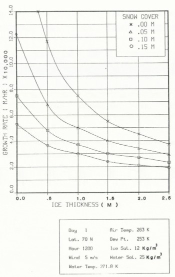
Fig. 7. Dependence of the ice-growth rate on snow cover and ice thickness.
3.3 Air temperature, solar radiation, and ice-growth rates
The impact of the air temperature on ice-growth rate produced by the model is, as should be expected, substantial (Fig. 8). At 0.5 m ice thickness, zero snow cover, and air temperature of 263 K, one finds a mere 0.001 m/h ice-growth rate. As the air temperature drops to 233 K the ice-growth rate increases to 2.5 times that value, which is not too dissimilar to that given by Reference Thorndike, Thorndike, Rothrock, Maykut and ColonyThorndike and others (1975) for the same time of the year.

Fig. 8. Dependence of the ice-growth rate on the air temperature and on ice thickness.
The effect of the solar radiation on the ice-growth rate, as produced by the model, is shown in Figure 9. By way of comparison, a winter and a summer day (Julian day 1 and 200) are selected. The latitude is set at 72°N. Zero snow cover is assumed. Selecting the 0.5 m ice thickness, one finds that in the winter night the growth rate of the ice is approximately twice that in summer day.

Fig. 9. Dependence of the ice-growth rate on solar radiation and on ice thickness.
3.4 Wind speed, ice temperature, and ice-growth rate
The effect of the wind speed on the ice-surface temperature and on the ice-growth rate may be studied by the application of Equations (39), (43), and (47), and of the assumptions made in its derivation. The vertical profile of the temperature in the ice, as produced by the model in response to atmospheric conditions, is shown in Figures 10 and 11, and the ice-growth rates are given in Figures 12 and 13. The impact of the wind speed is studied during a summer and a winter day, and under various snow depth covering the sea ice. For the sake of comparison, the air temperature and the dew point are kept constant in these runs: (T,TD) = (250,230) K (Figs 10 and 11).

Fig. 10. Dependence of the temperature of a snow-free ice surface on the surface wind.

Fig. 11. Dependence of the temperature of a snow-covered ice surface on the wind speed for a summer and a winter day.

Fig. 12. Dependence of the ice-growth rate on the ice thickness and on wind speed for a summer and a winter day.

Fig. 13. Dependence of the ice-growth rate on the ice thickness and on the wind speed (summer day, ice snow-covered).
Broadly, in terms of the vertical temperature profile in the ice and its growth rate, the model’s responses are:
-
(a) The thinner the ice, the more the ice-surface temperature approaches that of the ocean (272 K) for both wind speeds. This same conclusion can be inferred from Equation (48).
-
(b) Under the same oceanic and atmospheric conditions, thinner ice grows more rapidly than thicker ice (Fig. 12). This is in agreement with the results of Reference Thorndike, Thorndike, Rothrock, Maykut and ColonyThorndike and others (1975).
-
(c) The larger the wind speed, the lower is the ice-surface temperature produced by the model (Fig. 10). In view of the dependence of the heat and moisture exchange coefficients (Equations (39)–(43)) on the surface wind speed, this response can be derived from basic physical principles.
-
(d) The stronger the wind, the larger is the ice-growth rate (see Figs 11 and 12). This response is traceable to the physical processes described by Equations (39)–(43) and (11). Suffice it to add that the increase in heat loss by the ice surface with increasing wind causes larger thermal gradients in the ice which, in turn, increases the ice-growth rate.
Next, the effects of snow cover on the ice vertical temperature profile and on the ice-growth rate is examined for the two wind speeds.
Broadly, the main responses of the model are:
-
(e) The low thermal conductivity of the snow and the loss by the latter of heat through the sensible- and latent-heat fluxes result in the ice-surface temperature being substantially higher than when no snow covets the ice surface (Reference GeigerGeiger, 1965, p. 205–10).
-
(f) This insulating effect is also expressed in a smaller gradient of temperature in the ice and by Equation (11) in smaller ice-growth rates for both wind speeds. In particular, the temperature profiles in the ice produced by the model for both wind speeds do not differ substantially from one another (Figs 12 and 13).
To conclude, this diagnostic assessment has shown that the model is self-consistent, it responds reasonably well to atmospheric and oceanic forcing, and that its results are fairly comparable with those from other studies.
The viability of the model in predicting the sea-ice evolution over a fairly long time-scale is next examined.
4. Simulation of Sea-Ice Climatology
To test the extent of the numerical stability of the model’s algorithms and its ability to simulate the climatology of the first-year ice, three Arctic locations were chosen. These are: Frobisher Bay (lat. 63° 45′ N., long. 68°33′ W.), Cambridge Bay (lat. 69° 06′ N., long. 105° 07′ W.), and Alert Inlet (lat. 82° 30′ N., long. 62° 20′ W.) (Fig. 14). The choice was also based on the need to test the model at sites with diverse geographic, oceanic, and sea-ice climatologic characteristics (i.e. bay depth and its orientation, heights of tides, tidal currents, sea-ice seasonal accumulation, freeze-up, and total melt dates).

Fig. 14. The eastern Canadian Arctic showing Frobisher Bay, Cambridge Bay, and Alert Inlet.
4.1 Input data sources
The data required to run the model (Appendix) were extracted mainly from:
-
(1) Climate normals (1951–1980), Vol. 8. Downsview, Ontario, Environment Canada, 1984.
-
(2) Temperature and precipitation (the North), 1951–1980. Downsview, Ontario, Environment Canada, 1982.
-
(3) Water temperature and salinity at Cambridge Bay (1954–1967), Frobisher Bay (1951–1976), Alert Inlet (1967–1975). Downsview, Ontario, Fisheries and Marine Services, Environment Canada, 1980.
-
(4) Climatological studies. 1965, No. 3. Snow cover, Downsview, Ontario, Environment Canada, 1965.
-
(5) Monthly means of the oceanic flux F w (Appendix), initially based on Reference Maykut and UntersteinerMaykut and Untersteiner (1971) were modified to take into account the decrease in the thermal lapse-rate due to tidal mixing.
-
(6) Sea-ice thicknesses were extracted from Reference AllenAllen (1977) and processed in a manner described next.
4.2 Reduction of the sea-ice data
The original climatological sea-ice data set obtained from Reference AllenAllen (1977) was compiled into weekly averages of sea ice thickness in which the averaging number used was the total of the cases in which sea ice was actually observed Now, while for the middle of the sea-ice seasor the total of these events is nearly equal to the total of years of data availability (i.e. 26 years), the number of cases of early freeze-ups and late melts is much smaller and is located at either end of the sea-ice season. Thus the averaging technique used by Reference AllenAllen (1977) statistically emphasizes unduly these singular events; it stretches artificially the sea-ice season and it introduces distortions into the climatological trend of the seasonal sea-ice thickness. For example, Figure 15 shows a relatively high peak in the ice-thickness graph in mid-July, at the height of the melt season. This peak is traced to a single occurrence in the 26 years of data and one in which broken ice was transported northward to Frobisher Bay by persistent southerly winds during the week of 9–15 July. Similar, but less pronounced peaks, were found in the Alert Inlet and Cambridge Bay data (not shown in this paper).

Fig. 15. Ice thickness for Frobisher Bay extracted from the average weekly records (——); broken lines (----- ) indicate ice thickness after data reduction; dotted lines (….) show standard deviations.
Another type of forcing which can locally have considerable effect on the date of freeze-up and break-up is due to oceanic tides. Often, the onset of the sea-ice season is preceded by the breaking up of newly formed ice by wind waves, swells, and tides. This process, which can recur several tunes before the sea-ice season is finally established, delays the freeze-over date. This tide-enhanced delay was parameterized in our model by increasing the depth of the oceanic mixed layer. By contrast, the break-up of newly formed ice by the oceanic waves falls within the higher frequency mode of the synoptic scale. The averaging technique adopted by Reference AllenAllen (1977), then, tends to emphasize these scales particularly at the beginning and towards the end of the ice season (Fig. 15). Thus, for the climatological thermodynamic trend to be more clearly seen and compared with the model’s output, it is necessary to identify and eliminate these higher frequency modes. Accordingly, the dates of freeze-up and of total melt appearing in the weekly based climatological data (see for example Figure 15) were modified slightly by extrapolating linearly from the third week in which ice was first observed to the point where the accumulated sea-ice thickness curves intersect the zero ice-thickness lines. These curves were similarly adjusted prior to total observed melt. As is evident from Figure 15, these adjustments are minor, particularly during the ice-accretion period. In addition, the method was found capable of eliminating the climatologically unacceptable features of peaks in ice-thickness curves during the melt season and zero ice-accretion rates following freeze-ups found in the initial input data (Fig. 15).
4.3 Output verification in climatology simulation
The climatological simulation by the model of the yearly cycle was initialized on 1 August and run for 13 consecutive months.
Starting with open-water conditions, the model produces hourly changes in temperature and in salinity in the oceanic mixed layer leading to freeze-up. Following freeze-up, the model produces hourly rates of ice accretion, the total accumulated ice, the date of initial melt, the ice-ablation rate, and the date of open-water conditions.
The adjusted climatology of the first-year ice and the corresponding simulation by the model for the three Arctic locations under study are shown in Figures 16, 17, and 18. These graphs also serve as the basis to assess the model’s performance. Parameters used in the comparative analysis are: the maximum seasonal sea-ice thickness, the length of the ice-accretion and ice-ablation periods, ice-accretion and ice-ablation rates, dates of freeze-up, and of the onset of open-water conditions.

Fig. 16. Ice thickness for Frobisher Bay: model, climatology, and Thorndike and others.

Fig. 17. Ice thickness for Cambridge Bay: model, climatology, and Thorndike and others.

Fig. 18. Ice thickness for Alert Inlet: model, climatology, and Thorndike and others.
A note of caution is in order. While the average ice-ablation rate can be roughly defined as that ratio obtained by dividing the amount of the ice melted by the period during which this melt has occurred, a fundamental flaw may exist if, for the first-year ice, such a definition is carried beyond a fairly long period of substantial ice melt. Roughly, and depending on the initial thickness of the ice and its physical properties, it is at this point in time that the non-thermodynamic effects may become very important contributions to the seasonal change in the sea-ice thickness. Mainly, these processes are: the deterioration of the sea ice which generally accompanies the ice melt and which causes a decrease in its strength, the flexural torque and the break-up of the sea ice by waves and tides, and, finally, the removal of the broken-up ice by surface winds. These are the processes which contribute to the abrupt change noticeable in Figure 15 in the third week following the initial melt. This point will be further elaborated upon in the concluding remarks.
4.4 Maximum seasonal ice thickness
The maximum seasonal ice thickness produced by the model at the three Arctic locations differs from the corresponding climatological value by 10% or less (Figs 16–18). For Frobisher Bay, the difference is less than 5%. Particularly faithfully reproduced by the model is the difference that exists in this parameter from one location to another. By way of illustration, the minimum value in the seasonal ice thickness occurs in Frobisher Bay. Alert Inlet and Cambridge Bay have comparable thicknesses. Both the minimum at Frobisher Bay and the comparable quantities at the other stations are very well simulated by the model.
4.5 Length of ice-accretion period
In general, the climatological curves (Figs 16–18) show that the period of ice accretion is substantially longer than that of ice ablation. The model simulates this very faithfully. In addition, for all the three locations, the difference in the dates of maximum seasonal ice thickness, as produced by the model vis-à-vis the corresponding climatological value, falls well within the time resolution of 1 week inherent to the data base.
4.6 Length of the ice-ablation period
For Frobisher Bay and for Cambridge Bay (Figs 16 and 17), the length of the ice-ablation period produced by the model is in very good agreement with the corresponding climatological value. For Alert Inlet (Fig. 18), a difference of approximately 2 weeks is discerned. In addition, a change in the ablation rate is found for Frobisher Bay and for Cambridge Bay approximately 2 weeks prior to the onset of open-water conditions in the climatological curve. Such a difference is not produced by the model. An explanation of the source of these differences is given in the concluding remarks later in this paper.
4.7 Ice-accretion rate
The initialization procedure used by Reference AndersonAnderson (1961) to avoid numerical instability in the calculation of the ice-accretion rate at small ice thickness
4.8 Ice-ablation rate
Figures 16, 17, and 18 show that the ablation rate produced by the model in the first 3 weeks of ice ablation is realistic. In particular, for Frobisher Bay and Cambridge Bay the climatological and modeled average ablation rates are in very good agreement throughout the entire melt period. For Alert Inlet, however, the model produced, on average, ablation rates which are smaller than the corresponding climatological value. This point will also be analyzed later in the paper.
4.9 Freeze-up dates
The difference between model-produced and climatological freeze-up dates (Figs 16–18) is well within the resolution provided by the frequency of data availability. In particular, for Frobisher Bay and for Cambridge Bay, the correspondence is excellent. Particularly significant is the good reproduction by the model of the difference in the freeze-up dates which exists between the three Arctic locations under study. For Alert Inlet, this is found to be in early September, for Cambridge Bay it is in early October, and for Frobisher Bay in early November.
4.10 The onset of open-water conditions
Comparison between the dates of the onset of open-water conditions as produced by the model vis-ὰ-vis the corresponding climatological dates shows that very good correspondence exists for Frobisher Bay and Cambridge Bay (Figs 16 and 17), while for Alert Inlet (Fig. 18) the model is about 2 weeks late in predicting the event.
4.11 Comparison between sea-ice models
Compared with both climatology and this model (Figs 16–18), Reference Thorndike, Thorndike, Rothrock, Maykut and ColonyThorndike and others’ (1975) growth rates, at 1 m ice thickness or less, are found to be unrealistically large. Similarly, at 1 m ice thickness or more, Thorndike and others’ growth rates are found to be substantially smaller than those obtained from this model or from climatological data.
In addition, the seasonal maximum sea-ice accumulation is found from Thorndike and others’ table to occur substantially later. This deficiency has the further effect of maintaining the sea ice through the entire year. This is contrary to the observed open-water conditions which occur during summer.
Turning next to Anderson’s equation, its application in this study has been found to be useful following freeze-up and ice thicknesses of up 0.10 m. Despite this usefulness, Anderson’s Equation (46) breaks down whenever the air temperature becomes equal to the water-surface temperature, regardless of the solar-radiation flux. In addition to this deficiency, Anderson’s equation was derived under the assumption of no explicit snow cover.
5. Conclusion
The sensitivity tests with this model and its subsequent application to three Arctic locations have fairly conclusively shown its potential applicability as a predictive tool.
The elaborate treatment of the short-wave radiation, the impact of cloudiness on the latter, and of the albedo of the different surfaces have contributed to the good performance of the model, The impact of cloudiness on the long-wave radiation formulation remains to be adequately treated. Work is under way to derive some climatological values of cloud ceilings and their water content for the Arctic. The model has also highlighted the importance of the solar-radiation scattering process in the ocean, in the ice and in snow.
The inclusion of tidal mixing in the oceanic mixed layer, though crude, has proven its effectiveness in the prediction of the freeze-up date. The need of a more systematic formulation of this process remains.
The removal of the high-frequency mode in the yearly cycle of the sea ice (Fig. 15), though applicable in climatological studies, has highlighted the importance of other physical processes. Broadly, these are: melt percolation in the ice, the deterioration of sea ice due to melt, and the break-up of sea ice by flexural stress caused by ocean swell (Reference WadhamsWadhams, 1973; Reference Squire, Allan and PritchardSquire and Allan, 1980; Reference Ashton and LunardiniAshton, 1984), A study of the impact of these processes is presently under way.
Finally, more observational evidence is required to assess adequately any formulation of the evolution of brine pockets in the ice and of the oceanic heat flux.
Appendix
Meteorological and oceanographic climatology input data


