

1. INTRODUCTION
The changing extent and increased seasonality of Arctic sea ice due to anthropogenic climate change will have important effects on feedback mechanisms within the Earth's climate system (IPCC, Reference Pachauri and Meyer2014). Not only is the areal extent of Arctic sea-ice cover diminishing in summer, but the composition of that ice is also changing; as the sea ice becomes more seasonal rather than perennial, larger amounts of first-year ice are present compared with multi-year ice (Weeks, Reference Weeks2010; Maslanik and others, Reference Maslanik, Stroeve, Fowler and Emery2011).
These changes will be important as the rejection of brine from growing and decaying sea ice influences the distribution of salt in the ocean and therefore global thermohaline circulation (Gill, Reference Gill1973; Aagaard and others, Reference Aagaard, Coachman and Carmack1981; Morison and others, Reference Morison, McPhee and Muench1993; Ohshima and others, Reference Ohshima2013), while nutrients and dissolved gases are entrained in the moving brine and sea water (Vancoppenolle and others, Reference Vancoppenolle2013; Zhou and others, Reference Zhou2013). Therefore, the identification of mechanisms involving brine transport, and how they change under different conditions, is necessary to allow a better understanding of the possible effects on ocean circulation, the evolving sources and sinks of climatically important gases such as carbon dioxide, and of the nutrient cycle and algal concentrations within the sea ice (Notz and Worster, Reference Notz and Worster2009; Wells and others, Reference Wells, Wettlaufer and Orszag2011; Jardon and others, Reference Jardon2013).
The mechanisms of sea-ice formation have been well described previously: as pure ice freezes from sea water, the salts initially dissolved in the water are expelled from the ice crystals. As the bulk ice layer grows, dissolved salt remains trapped within the liquid inclusions of increasingly saline brine. However, it has been known for a long time that bulk sea ice is less saline than sea water (Weeks and Ackley, Reference Weeks, Ackley and Untersteiner1986; Weeks, Reference Weeks2010), and therefore that most of the salt is removed from the system over time. Previous observations have proposed that desalination of sea ice takes place through a variety of mechanisms during its growth and decay: e.g. salt segregation at the growing ice–ocean interface, brine diffusion, brine expulsion, gravity drainage and flushing (Cox and Weeks, Reference Cox and Weeks1975; Weeks and Ackley, Reference Weeks, Ackley and Untersteiner1986; Notz and Worster, Reference Notz and Worster2009; Weeks, Reference Weeks2010 and references therein).
For the sake of clarity, we will briefly redefine here some of these processes and associated terminology: (1) salt segregation at the growing ice/ocean interface (‘initial entrapment’ in Weeks and Ackley, Reference Weeks, Ackley and Untersteiner1986 and Weeks, Reference Weeks2010) refers to a process by which most of the salts are rejected from the newly growing pure ice crystals, along the ice/water interface due to the fact that the crystal lattice can only accommodate a limited amount of impurity. This process increases the salt concentration (and therefore water density) in the interfacial boundary layer below the ice/water interface. The difference in concentration drives both diffusion of the salt toward the less saline bulk sea water and buoyancy-driven interfacial convection in the water below the interface. (2) Gravity drainage, as defined by Eide and Martin (Reference Eide and Martin1975), refers to processes within the ice layer caused by the fact that the greater density of the brine relative to that of the sea water drives the brine down and out of the ice into the underlying sea water. From mass balance considerations, gravity drainage also implies upwelling of sea water compensating for the brine loss. Such convection in the ice generally occurs as the ice cools from the top, and some of the liquid in the brine inclusions freezes as pure ice, increasing the salinity (density) of the remaining brine. Provided that the brine network is sufficiently interconnected, a buoyancy-driven instability will initiate the downward drainage process within brine channel structures. These conditions will typically occur continuously in the lower centimeters of actively growing sea ice (Notz and Worster, Reference Notz and Worster2008), or episodically throughout the sea ice cover on Spring warming (e.g. Jardon and others, Reference Jardon2013; Zhou and others, Reference Zhou2013 and references therein).
The structure of sea ice has also been described as a mushy layer: ‘a rigid matrix of pure solid (ice) bathed in its impurity rich melt (brine)’ (Feltham and others, Reference Feltham, Untersteiner, Wettlaufer and Worster2006). This structure is not unique to sea ice, but is also found in other solidifying systems, e.g. metallic alloys (Worster, Reference Worster1991, Reference Worster1997; Tait and others, Reference Tait, Jahrling and Jaupart1992; Chen, Reference Chen1995). A ‘mushy layer’ can be considered as a dynamic heterogeneous medium, in which the melt phase can move in the gravity field as the solidification interface migrates away from the heat sink. Extensive experimental and theoretical works on directional solidification of metallic alloys and equivalent media such as aqueous ammonium chloride solutions have led to a well-developed theory of convection during mushy layer evolution (Worster, Reference Worster1992, Reference Worster1997 and references therein).
It is now understood that two independent buoyancy-driven modes of convection can develop: (1) the large-scale mushy-layer mode, which leads to convection inside the mushy zone, responsible for the occurrence of chimneys and defects in alloys, and of brine channels in sea ice, and (2) the small-scale boundary-layer mode, induced by unstable density profiles (local denser region above a less dense region) in a boundary layer zone inside the liquid phase close to the solid/liquid interface. This mode leads to smaller size convection in the liquid, which does not change the solid fraction distribution inside the mushy layer. Either mode can be the dominant mode depending on the values of the describing parameters. In this mushy layer description for sea ice, the interfacial boundary layer convection mode corresponds to the so-called salt segregation, while the mushy layer mode is that responsible for gravity drainage.
The mushy layer theory has been successfully applied to brine transport within sea ice (see e.g. the review by Hunke and others, Reference Hunke, Notz, Turner and Vancoppenolle2011). The discussion of Notz and Worster (Reference Notz and Worster2009) concluded, in accordance with previous work that (of the set of mechanisms described above) the dominant mechanisms of salt flux to the ocean are gravity drainage through the brine channels during growth and flushing during melting.
In the field, brine channel drainage structures, indicative of internal convection, have been observed (e.g. Lake and Lewis, Reference Lake and Lewis1970; Wettlaufer and others, Reference Wettlaufer, Worster and Huppert1997; Weeks, Reference Weeks2010), but studies of the brine content of ice cores are hampered by draining during collection (Notz and Worster, Reference Notz and Worster2009). Avoiding this problem, in situ measurements in growing sea ice have enabled time-dependent measurements of the evolution of the ice bulk salinity at different depths to be made (Notz and others, Reference Notz, Wettlaufer and Worster2005; Notz and Worster, Reference Notz and Worster2008). These measurements led to the conclusion that no segregation could be observed in the melt at the mushy layer–liquid interface (at least at the scale of the measurements) therefore suggesting that salt segregation at the interface is not a significant desalination process (Notz and Worster, Reference Notz and Worster2009). Although these measurements have added much needed quantification to these processes, there are still unknowns associated with these methods. The measurements give an average salinity at each given depth over tens of centimeters, which does not, therefore, allow consideration of the finer internal structure of the ice. An important qualification made by Notz and others (Reference Notz, Wettlaufer and Worster2005) is that the resolution of their measurements may be lower than necessary to observe the salinity increases below the interface.
In more controlled conditions, laboratory studies have been performed in 3-D tank experiments. In these experiments, salt water is cooled from above to replicate conditions during natural sea-ice formation, and the brine rejection processes are observed or measured. In the work of Cottier and others (Reference Cottier, Eicken and Wadhams1999), ice was grown in a large, meter scale tank, and sampling of the ice was combined with high-resolution measurements of salinity. These results show that brine channel structures are associated with localized increased salinity below them in the underlying water, and significant brine depletion in the ice surrounding these channels, thereby showing that the brine channels are a major path for brine rejection in growing sea ice. Experiments in smaller scale tanks have also been conducted, allowing tighter controls on the starting parameters of experiments and higher resolution observations. For example, the work of Wakatsuchi and Kawamura (Reference Wakatsuchi and Kawamura1987) has shown that brine channel position may be controlled by the ice crystal structure, and that brine pockets move between the intercrystalline lamellae. Sampling underneath the ice layer has also shown that the salinity and volume flux of brine rejections is dependent on the ice growth rate (Wakatsuchi and Ono, Reference Wakatsuchi and Ono1983; Wakatsuchi, Reference Wakatsuchi1984).
Experiments combining visual observations of the evolving ice/water interface and brine dynamics with measurements in the water layer have also been carried out. Wakatsuchi (Reference Wakatsuchi1984) used Schlieren imaging methods to visualize the movement of brine under a growing sea-ice layer, observing fine sinking brine streamers whose dynamics were dependent on the growth rate of the ice. Wettlaufer and others (Reference Wettlaufer, Worster and Huppert1997) combined shadowgraph observations of brine rejection in the water layer with measurements of salinity and temperature in the bulk water reservoir in their tank. These authors observed two distinct sets of streamers during ice growth: earlier weaker streamers interpreted as being ejected by interfacial convection, and later, stronger streamers interpreted as internally driven convection, resulting in a detectable increase of the bulk water salinity.
The images obtained by Schlieren and shadowgraphy methods in experiments such as these result from the projection of 3-D information onto a 2-D plane, therefore the interpretation of these results is sometimes difficult. All the 3-D experiments also suffer from the important drawback that internal structure in the ice can only be investigated after growth in post-mortem investigations. Aussillous and others (Reference Aussillous, Sederman, Gladden, Huppert and Worster2006) combated this problem during growth of a mushy layer in an aqueous sucrose solution using magnetic resonance imaging. Similarly, Chen (Reference Chen1995) mapped the internal structure of a solidifying aqueous ammonium chloride solution using X-ray tomography. However, these (and similar) methods can only show information on the dynamics in the mushy layer, and connections to what happens in the liquid layer must be extrapolated (e.g. Wettlaufer and others, Reference Wettlaufer, Worster and Huppert1997).
Along with X-ray tomography, Chen (Reference Chen1995) used injection of a dye at discrete intervals as an easy method to follow transport processes in solidifying aqueous ammonium chloride solutions. Depending on the experimental parameters used, both interfacial and mushy layer modes of convection were visualized by tracing the dye motion. Movement of the dye within the mushy layer zone due to the fact that it has a density different than that of the interstitial liquid was also evidenced. The monitoring of interfacial convection could not be visually followed through time, given the dye penetration in the mushy layer, but repetition of dye injection at a later stage of growth (when chimneys were already active) again showed interfacial finger convection. Disadvantages inherent to this method are, however, the inability to continuously track the dynamics, the low resolution of the boundary convection tracking and also the potentially active influence of density of the dye on the buoyancy-driven convective processes.
One option which allows visualization directly through the solid layer is the use of a quasi-2-D tank. Chen (Reference Chen1995) used this method to visualize within a mushy layer formed from aqueous ammonium chloride, while Eide and Martin (Reference Eide and Martin1975), as well as Niedrauer and Martin (Reference Niedrauer and Martin1979), pioneered this method to analyze sea-ice growth, visualizing processes above and below the ice/water interface with the aid of a dye. Due to the dye introduced, brine plumes were visualized sinking into the water from brine channels in the ice (Eide and Martin, Reference Eide and Martin1975). Niedrauer and Martin (Reference Niedrauer and Martin1979) also observed dye rising into the mushy layer, fresher water rising to replace the rejected brine, an equivalent observation to the movement of dye observed by Chen (Reference Chen1995) in the ammonium chloride system. Occasionally, upward flow of fresher water has been reported as occurring in the brine channels themselves, where a switching mechanism, including an evolving geometry of the channels, operates to control downward and upward flows (Eide and Martin, Reference Eide and Martin1975). This switching is thought to be similar to the ‘salt oscillator’ of Martin (Reference Martin1970), where the downward flow competes with the upward buoyancy force. As flow continues, the structure of the channel changes, so changing the ratio of downward-to-upward buoyancy factors, allowing the less dense water upwelling to override the denser salt-driven downwelling (Weeks, Reference Weeks2010).
However, as already suggested by Chen (Reference Chen1995), the use of a dye to enhance the visualization of the flow and the entrainment of liquids may in itself affect the dynamics of the system. Niedrauer and Martin (Reference Niedrauer and Martin1979) specifically state that in their experiment the negative buoyancy of the dye with respect to the sea water enables it to rise to the interface to be entrained in the ice layer, without then considering whether that negative buoyancy has an effect on their observations within the ice. More recent work in fluid dynamics has demonstrated that the introduction of a colorant can in fact change buoyancy-driven flows, and should therefore be used with caution (Almarcha and others, Reference Almarcha2010; Kuster and others, Reference Kuster2011; Thomas and others, Reference Thomas, Lemaigre, Zalts, D'Onofrio and De Wit2015).
From the above literature survey, it is clear that there are still a certain number of unknowns concerning impurity transport processes within the sea-ice system. In particular, there is no combined approach that simultaneously follows the processes occurring both within and underneath the ice layer, at a high resolution, without the addition of an external compound, which may affect the observations. In this context, we present here two adaptations of non-invasive optical Schlieren imaging methods used to visualize brine channel development and convective processes during ice growth in a quasi-2-D ice–salt water system. These methods: (1) allow visualization of the processes present, at a high spatial resolution, without introducing a perturbing dye, (2) allow continuous observation of all processes simultaneously within the sea-ice layer and in the water, and (3) show, in situ, the links between the convective dynamics in ice and in water. These techniques pave the way to a non-invasive high-resolution characterization of sea-ice growth dynamics, which will be useful for future quantitative comparison with modeling.
The paper is organized as follows: first, in Section 2, we present the experimental setup and methods: a Hele-Shaw cell (Section 2.1) and a description of Schlieren imaging, which allows visualization of density differences (Section 2.2). Two visualization methods are used: a traditional Z-type Schlieren imaging system (Section 2.3) and a synthetic Schlieren imaging system (Section 2.4). Then the results are presented in Section 3, with descriptions of the major observations made. A discussion of the observational methods and the results obtained, including an evaluation of the limitations of the visualization systems, is found in Section 4. In Section 5, we summarize the conclusions from this study and the challenges which remain.
2. EXPERIMENTAL METHODS
2.1. Hele–Shaw cell
To visualize the convective flows and the evolution of structures within a growing sea-ice layer, we use a quasi-2-D experimental setup known as a Hele-Shaw cell, similar to that previously used by, e.g. Eide and Martin (Reference Eide and Martin1975) or Chen (Reference Chen1995). The cell consists of two vertically oriented, parallel Plexiglas plates of thickness 10 mm, separated by a small gap. The space inside the cell has a vertical height of 64 cm, a horizontal width in the plane of the images of 34 cm, and a depth (perpendicular to the plane of the images, i.e. parallel to the light path) of 3 mm. Throughout this paper, the vertical growth of the ice will be referred to as the thickness of the ice. An expansion burette is attached to an outlet at the base of the cell, so allowing water to leave the cell as ice freezes, avoiding an increase in internal pressure.
The cell is filled with an aqueous NaCl solution of starting concentration 35 ppt, and is mounted within an optical imaging system in a temperature controlled environment. We apply a vertical temperature gradient to the cell by flowing alcohol at a fixed temperature through its lid. This alcohol is in contact with a copper plate, which is in turn in contact with the cell, so transmitting the controlled temperature and cooling the cell from above. With a lid temperature below the ice freezing point, a quasi-2-D model of the freezing front, which develops in natural sea ice, can then form as ice grows downwards from the cooled lid. As salt is rejected from the ice layer, the salinity in the remaining water will increase, so changing the dynamics of the system. However, as we are here interested in the visual observations that are possible, we do not consider the ramifications of this salinity increase further, although it would be important to include in full quantitative studies.
The use of a Hele–Shaw cell, although an advantage for imaging purposes as it allows light to pass through the ice, has certain potential drawbacks: the inherently 3-D process of brine channel formation (Lake and Lewis, Reference Lake and Lewis1970; Galley and others, Reference Galley2015) is confined in a quasi-2-D geometry. A discussion of the advantages and disadvantages of this method will be presented in Section 4.6 in connection with the results obtained.
2.2. Schlieren imaging
In order to image the movement of brine both within the ice and under the ice/water interface at high resolution, we use Schlieren visualization techniques. Schlieren methods exploit the fact that the physical properties of a liquid affect its optical properties, in particular its refractive index. By observing the effect of these refractive differences on light rays which are shone through the cell, we are able to visualize areas of different composition. We can therefore observe the downward flow of denser brine through fresher water as the sea-ice freezing front progresses.
A quasi-2-D system, as used here, inhibits superposition of brine streamer information, while also allowing simultaneous observation within the ice layer (impossible in visualization of 3-D systems). Large improvements in camera and computer technology also allow us to increase the spatial resolution of Schlieren images compared with previous work. Two distinct Schlieren techniques have been used in this study: traditional Schlieren imaging (Settles, Reference Settles2001) and synthetic Schlieren imaging (also known as background-oriented Schlieren imaging) (Dalziel and others, Reference Dalziel, Hughes and Sutherland2000). We will discuss the detailed methodology of these two techniques separately.
2.3. Traditional Schlieren imaging
As the composition and temperature of a liquid influences its refractive index, a gradient of salinity will generate a gradient of refractive index. A passing light ray will therefore be refracted, as seen in Figure 1, the degree of refraction being proportional to the local gradient of refractive index. The traditional Schlieren imaging system captures this refraction through the use of two parabolic mirrors mounted in a Z-type configuration (Wakatsuchi, Reference Wakatsuchi1984; Settles, Reference Settles2001). A light-emitting diode light source (LED in Figure 1) illuminates a slit placed at the focal distance of the first mirror (Fig. 1), and the resultant parallel rays pass perpendicularly through the area of interest (our Hele–Shaw cell). Unperturbed rays which continue parallel are refocused by the second mirror, at this second focal point a razor blade is positioned such that half of these rays are blocked. Therefore, any light rays that have been deviated from parallel due to the gradients of refractive index induced by the dynamical processes inside the Hele-Shaw cell are either fully blocked, or pass the razor (Fig. 2). A video camera is placed behind the razor blade, allowing digital images of the cell to be taken at controlled intervals during experiments. Gradients in the refractive index are therefore imaged directly in the digital photos as changes in luminosity, and density differences can be inferred. These images are enhanced in post-processing by subtracting a reference image, which is taken before cooling begins, then adjusting the brightness and contrast of the resulting images to best highlight the dynamics, which develop below the ice. The enhancement process has various advantages: uneven light distribution can be balanced, and marks or scratches on the cell are minimized (due to their interaction with the changing light, they cannot be removed entirely).
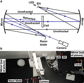
Fig. 1. Traditional Z-type parabolic mirror Schlieren assembly: (a) Schematic showing light paths of parallel rays (solid lines) and rays that are refracted by a refractive index gradient within the Hele–Shaw cell (dashed lines); (b) Adapted Schlieren assembly in an environmental chamber, set up as that of the schematic. The additional torch is used for extra illumination through the ice in the ‘adapted Schlieren’ method; parabolic mirrors not shown.

Fig. 2. Detail of Figure 1, schematic of light paths between second mirror, razor blade, and camera. Parallel light is blocked by an amount proscribed by the placement of the razor blade (black and gray solid lines). Light disturbed by a refractive index gradient can either be refracted onto the blade (red dashed-dotted line), resulting in a darker area in the image, or refracted away from the blade (blue dashed line), resulting in a lighter area in the image.
Due to the low-level light required for Schlieren imaging, and because of the refraction of light by ice crystal boundaries, the ice layer is obscure in traditional Schlieren images. To improve observations of the brine channels in the growing ice layer, an additional light source (the torch seen in Fig. 1b), was added behind the ice layer and focused on the upper centimeters of the cell. This additional light beam was placed at a slight angle to the incident parallel rays and was directed above the ice/water interface, to avoid affecting the Schlieren imaging within the liquid. We refer to this method as the ‘adapted Schlieren’ method from here on.
2.4. Synthetic Schlieren imaging
A cheaper, and often simpler, method to visualize density differences and flow in liquids is synthetic (or background oriented) Schlieren imaging, where the spatiotemporal evolution of the refractive index in the cell is reconstructed from images taken of a pattern placed behind the cell. A random pattern of points is mounted in front of a lightpad and imaged through the Hele–Shaw cell, firstly before the experiment begins, as a reference image, then at regular intervals during the experiment (Fig. 3). As refractive index changes occur due to convection and density differences, light paths will deviate (Fig. 3a) and the pattern imaged by the camera will be deformed with comparison to the reference image. By tracking these changes and subtracting the reference image from the refracted image, the convective motions inside the cell can be reconstructed (Dalziel and others, Reference Dalziel, Hughes and Sutherland2000). The image is further improved by adjustment of the brightness and contrast of the subtracted image. To assess brine channel movements above the interface, and brine streamer movement below the interface, the processed and unprocessed images can be used together – unprocessed images allowing details within the ice layer to be observed, processed images highlighting movement in the underlying water.

Fig. 3. Synthetic Schlieren assembly: (a) Schematic of setup, showing unrefracted (solid lines) and refracted (dashed lines) light rays. (b) Apparatus in environmental chamber; camera, cell and lightpad are visible. The pattern that is imaged is only present at the top right-hand section of the light pad, to allow comparison between synthetic Schlieren imaging, and imaging of the ice growth with plain illumination from behind. (c) Close-up view with ice growing in top few centimeters of cell, pattern is present on the left-hand side of the light pad.
3. RESULTS
3.1. Observations with both traditional and synthetic Schlieren techniques
A diagram representing the two experimental paths, i.e. those of the traditional and synthetic Schlieren techniques, is shown in Figure 4. This figure shows the details of the imposed experimental conditions, the timing of each stage of the experiment, and the format of the results obtained.

Fig. 4. Schematic of experimental procedure for both traditional and synthetic Schlieren experiments. The timing of experiments, and a summary of the results presented in the rest of the paper are shown. Breaks in data collection due to adjustment of the optical systems are noted.
An example image obtained using the traditional Schlieren method is shown in Figure 5; a non-processed Schlieren image (Fig. 5a) is shown with the equivalent processed image (Fig. 5b) for comparison. The original cell temperature was set to −1 °C and cooling initiated from the top of the cell at a temperature of −20 °C. The top of the cell is ~1 cm above the observed field of view (FOV). In the original image, brine rejection features are visible sinking from the ice layer. By processing the image, these features become more obvious and further details become evident, such as their internal structure. Particularly apparent is the difference in the right-hand side of the FOV, where features that are not clearly visible in the unprocessed image due to uneven lighting become visible in the processed image. Figure 6 and Video 1 (supplementary material) show the evolution of the dynamics as imaged with the traditional Schlieren technique.

Fig. 5. Traditional Schlieren images of brine rejection from a growing ice layer. (a) Unprocessed image, ice is the dark area at the top of the image. Brine rejection is visible due to areas of differing luminosity, which outlines thin streamers sinking from the ice/water interface into the underlying water layer. (b) Processed image, normalized to a reference image (taken before cooling began) and enhanced in post-processing. More details of the streamers are visible. FOV is 9.5 cm × 12.5 cm.

Fig. 6. Time series of processed traditional Schlieren images during cooling and ice growth. The starting temperature of the cell was −1 °C, the temperature imposed at the top of the cell was −20 °C. Ice is visible as the dark area at top of image, which increases in thickness over time. Brine rejection features are visible under the ice layer, with short fingers (a) joined by longer streamers over time. The average distance between the streamers increases with time. Multiple generations of streamers are visible in (e) and (f), with more dissipated streamers (i.e. wider and less luminosity difference) followed by tighter streamers with higher luminosity differences. Highlighted features in (b–d) show mushroom shaped heads of the streamers, as well as merging and tip splitting events. The images are normalized by subtracting a reference image and the contrast enhanced in post-processing. FOV is 9.5 cm × 12.5 cm.
With the addition of an extra light source, as detailed in Section 2.3 (the adapted Schlieren technique), even more details become apparent. As seen in Figure 7 and Video 2 (supplementary material), the dynamics below the ice are still visible, but now we are able to simultaneously visualize within the ice layer, highlighting structures that develop (Section 3.4).
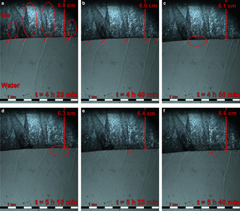
Fig. 7. Time series of adapted traditional Schlieren images of ice, with an additional torch illuminating the ice layer. The starting temperature of the cell was −1 °C, the temperature imposed at the top of the cell was −20 °C. Arrows in (a) show brine exit points from well-developed channel structures (circled). These channels are fairly stable in spacing, although there is some lateral movement of the exit points (e.g. an extra brine streamer has drifted in from the right-hand side of the image in (b), exit points indicated by arrows). Shorter brine rejections are visible between brine channels, becoming more apparent with time (circled areas in (c) and (d)). Arrows in (e) and (f) show the exit point of one brine channel from which brine stops flowing. The experiment imaged here is the same experiment as Figs 5 and 6. Due to the change in the optical imaging system, the first image was taken approximately 1 h 25 min after Fig. 6f. As the imaged FOV is at the top of the area illuminated by the circular mirror, some dark areas are visible at the top of the images, particularly the top right-hand corner, due to the limits of the mirror. FOV is 10 cm × 12.5 cm.
An experiment under the same conditions was carried out using the synthetic Schlieren technique. Example images obtained, using this method are shown in Figure 8, both before and after image processing. In the unprocessed images, some structure can be seen in the growing ice layer, which is lost in the processed image. However, under the ice/water interface, details, which were not apparent in the unprocessed image, have become visible: brine rejections sinking from the ice layer, discernable as white areas on the black background. These images do not show the brine features as clearly as the traditional Schlieren images, a point we will discuss further in Section 4.5.

Fig. 8. Time series of synthetic Schlieren images. Unprocessed (a, c, e) and processed (b, d, f) images. The starting temperature of the cell was −1 °C, the temperature imposed at the top of cell was −20 °C. Features in the ice layer, such as ice crystals and brine channels, are highlighted in the unprocessed images; features in the water layer are visible in the processed images. Brine streamer dynamics change during the course of the experiment, e.g. an extra streamer is circled forming between (d) and (f). Less well-defined rejections are visible between the larger streamers in (f) (right-hand oval). Arrows indicate the position of brine ejection points identified in (b, d, f), and seem to be related to the cross-cutting lamellae crystal structure identified in (a, c, e). The reference image for processing was taken 15 min after ice growth began and 45 min before (a, b). FOV is 4.3 cm × 4 cm.
3.2. Shallow reaching fingers
The brine rejections visualized using these methods manifest first as short fingers sinking from the cooled upper boundary (Fig. 6a, Video 1). These are visible from the top of the observed FOV (1 cm below the top of the cell) after ~20 min of cooling. These fingers are first seen at the left-hand side of the images, but this is likely to be an artifact of the imaging method, as the top right-hand corner is not imaged due to the shape of the parabolic mirror. After image processing, as described in Section 2.3 (Fig. 6), these fingers become much more obvious. Ice growth is visible as the dark area at the top of Figure 6b, which grows downwards in the next panels. The short fingers remain present throughout ice growth, independent of additional longer streamers, which appear later in the experiment (described in the next section). The fingers have a small wavelength of the order of 0.5 cm and extend in a short vertical convective zone that remains of the order of 1 or 2 cm throughout the experiment (Figs 6, 7; Videos 1, 2). These short fingers, clearly seen in videos, are not very well defined on the unprocessed static images (Figs 5a and 7), suggesting a low refractive index gradient between them and the surrounding salt water. There is also evidence of short, less well defined, rejection fingers at the interface, accompanied by longer streamers from the synthetic Schlieren imaging shown in Figure 8f (right oval). From the examination of images taken with the adapted traditional Schlieren technique (Fig. 7; Video 2), these short fingers do not seem to be associated with movement within the ice, but rather originate from the irregular-shaped interface in which the orientation of ice crystals is clearly visible.
3.3. Deep reaching streamers
After ~24 min of cooling, longer, more well-defined streamers emerge from the background of shorter fingers (Video 1; Fig. 6b). These brine streamers extend much further in the bulk water reservoir with time (tens of centimeters), some with distinctive mushroom shaped heads (Figs 6b and c). These streamers can also be seen to be well defined in the adapted Schlieren images (Fig. 7; Video 2), and are also visible in synthetic Schlieren observations (Fig. 8). The position and importance of these rejections vary with time, e.g. two streamers are present in the area highlighted in Figure 8f (left oval), whereas there was only one in Figure 8d (oval). Typical nonlinear dynamics of buoyancy-driven fingering such as merging, tip splitting and coarsening (e.g. Figs 6c and d) are observed. Rejection sites are approximately evenly spread across the ice width, and the distance between them increases with time (Videos 1 and 2; Section 3.5).
3.4. Brine channels inside the ice
Using the adapted Schlieren technique, the dynamics both above and below the interface can be connected (Fig. 7; Video 2). As well as ice crystal structures, such as intracrystalline lamellae, we are able to observe brine channel drainage structures (highlighted in Fig. 7a). These channels are associated with the long brine streamers identified in Section 3.3, brine originating from these drainage features being expelled in the long streamers. The structures in the overlying ice layer are more difficult to distinguish in the unprocessed synthetic Schlieren images than in the adapted Schlieren images, but a potential channel structure is also highlighted in Figure 8 (ovals in Figs 8c, e), which connects to the streamers highlighted in the processed images (ovals in Figs 8d, f). Close observation of the brine channel structures in Video 2 shows movement of ‘speckles’ – brighter spots which appear to move within the channel.
3.5. Streamer dynamics and ‘on/off’ behavior
The number of long streamers varies over the course of one experiment, and the average wavelength of the streamers increases with time (Figs 6, 7; especially clear in Videos 1 and 2). Therefore the overall position of the brine channels changes slowly with time. Analysis of the movement of one channel shows this drift to be on a timescale of ~0.02 mm min−1. Quantification of the change in number of streamers, and by implication brine channels, will be presented in Section 3.6.
The long streamers do not reject brine continuously. For instance, one streamer, sinking at the exit location of a brine channel observed in the ice (indicated by arrows in Figs 7e, f) can be seen to die out over time. Figure 9 shows the on/off behavior of this channel over a much shorter time period. This behavior is typical of the long streamers, some of which are seen to stop for a period of time, and then restart with a rapid ejection into the water layer (e.g. Video 2; t ≈ 6 h 30 min, central left finger; t ≈ 8 h, central right finger). Multiple generations of long streamers are seen over the course of time with, later, well-defined streamers following the same path as older, more dispersed, streamers (e.g. Figs 6e, f). Figure 10 shows this on/off behavior schematically for 5 of the major brine streamers that exist during the time period 4 h 10 min–8 h, where the local growth rate (ice thickness increase per unit time) ranges between 0 (just after cooling restarted at the beginning of the adapted Schlieren imaging) and 6.6 mm h−1. It can be seen that, for most of these streamers the ‘active’ period is longer than the ‘inactive’ period. Although the timings of these periods vary considerably between the fingers (e.g. streamer 5 is almost constantly active throughout the time period shown), the average activity of these five major streamers gives an ‘active’ period of 81% and ‘inactive’ period of 19% during this time window.

Fig. 9. Finer temporal resolution of brine streamer on/off behavior visualized with the adapted traditional Schlieren system. Arrows show a channel which is not releasing brine in (a), where a streamer begins to be visible in (b), and becomes stronger in (c and d). The streamer then slows and stops between (e) and (f). The dashed line in (a) shows the position of the ice/water interface in Fig. 7f. FOV is 10 cm × 12.5 cm.

Fig. 10. Schematic of streamer activity and local growth rate in the adapted traditional Schlieren experiment during the time period 4 h 10 min–8 h. Five representative streamers are shown, breaks in lines represent breaks in downwelling seen in images. There is a large range of ratios of activity (downwelling) and inactivity (inferred upwelling) between streamers.
3.6. Growth rate/streamers relationship
As mentioned in Section 3.5, the local growth rate of the ice thickness can be characterized from the images, along with other quantities such as the temporal evolution of the thickness of the ice layer, and the number of long brine streamers present in the 10 cm width of ice imaged in Figs 6 and 7. (We take long streamers to be those which persist at a depth of at least 2 cm below the ice layer, avoiding inclusion of the short fingers discussed in Section 3.2. We exclude the data from early in the experiment, where there are ambiguities in the number of streamers due to the shape of the mirror). The ice thickness increases with time (Fig. 11a), although the local growth rate diminishes with time (Fig. 11b) as expected from the insulation provided by the previously grown ice (decreasing the temperature gradient through the ice). In parallel, the number of streamers (Fig. 11c) decreases with time. The relationship between the local growth rate and number of streamers can be seen to be linear as a first approximation in Figure 11d. We discuss these results further in Section 4.3.

Fig. 11. Quantitative measurements from the traditional and adapted traditional Schlieren experiments: (a) ice thickness (mm), (b) local growth rate (mm h−1), (c) number of streamers per 10 cm ice width vs time (hours) and (d) number of streamers per 10 cm ice width vs local growth rate (mm h−1). Ice thickness increases with time, while local growth rate and the number of streamers decrease. The number of streamers correlates linearly to a first approximation with the local growth rate (thick solid line for linear regression). A representation of the relationship of Tison and Verbeke (Reference Tison and Verbeke2001) (adjusted for the different geometries used) is also plotted (thin black line). The break in data at time ≈ 5 hours in (a) is due to the adjustment of the optical system between traditional and adapted Schlieren methods, a corresponding drop seen in the growth rate is due to the resulting atmospheric warming in the environmental chamber.
3.7. Meandering of brine channels
In addition to the drift of brine channel position with time (Section 3.5), the local shape of the brine channels also changes. The channels show a meandering behavior as the ice grows, aiding to identify them in the videos (Figs 7 and 12; Video 2). Brine channel meandering can also be observed in Figure 12 and Video 3 (supplementary material), a zoom of one channel, imaged without the synthetic Schlieren pattern. We see that the channel ‘snakes’ within the ice layer and shows kinks that migrate both horizontally and vertically over time (~0.05 mm min−1 horizontally, 0.12 mm min−1 vertically). The kinks in the channel often orient quasi-parallel to the intracrystalline lamellae. New crystal growth is associated with the brine channel movements; as the ice layer grows, randomly oriented linear features can be seen to be concentrated around the position that the brine channel occupied (Figure 12; Video 3). The fine parallel intracrystalline structures at the right-hand side of the FOV are gradually replaced by these irregular features. The channel eventually stops moving and freezes after ~16 h. The replacement of lamellae by irregular features can also be seen in Video 2. The brine channel structure highlighted second from left in Figure 7a shows a cross-cutting relationship with the lamellar crystal structures in the ice. Over time, the parallel lamellae become more irregular, the light being refracted in more directions.

Fig. 12. Direct imaging of the temporal evolution of one brine channel. Arrows in the water layer show the exit point of the channel, which moves over time. Arrows in the ice layer show the joining point of two branches of the channel which also migrates, and a tight bend in the left-hand branch of the channel. The diagonally oriented lines visible on the right-hand side are ice lamellae similar to those seen in the ice in Fig. 7. In the area through which the channel migrates, these organized crystals have been replaced by recrystallization, shown by the randomly oriented black lines (crystal boundaries). FOV 1.7 cm × 7.9 cm.
3.8. Summary of main observations
To summarize, the main observations that can be made with the Schlieren techniques presented here are:
-
(1) Adapting the traditional Schlieren optical method with the addition of an extra light source allows simultaneous visualization of transport processes within the sea-ice layer, and in the water below the interface, giving more information than previously seen in Schlieren images of growing sea ice.
-
(2) Movement within the brine channels is shown by ‘speckles,’ changes in the luminosity within the channels that may be useful for future quantification of internal brine flow rates.
-
(3) Synthetic Schlieren imaging, not previously applied to sea-ice growth, allows observations of structures in ice and of rejected brine underneath the ice layer, after processing of images.
-
(4) Short convection fingers, which are not connected to the channels observed, persist throughout observations made with the traditional Schlieren method.
-
(5) Brine channel structures are observed within the ice layer, along with the associated long streamers that emanate from the channels into the underlying water layer.
-
(6) Long streamers emanating from the brine channels demonstrate on/off behavior.
-
(7) The number of long brine streamers and the local growth rate of the ice both decrease as the ice thickness increases. The number of streamers correlates linearly with the local growth rate.
-
(8) The average ice growth rate over an ice thickness of 10 cm is not necessarily representative of the local growth rate, which has been shown to vary widely in this experiment.
-
(9) Brine channels meander from side-to-side over time, following the intracrystalline microstructure.
4. DISCUSSION
With regard to the visualization of processes, we have shown that observations under the water layer can be improved when compared with the previous imaging studies, and also combined with observations above the interface by using both ‘adapted traditional Schlieren’ and synthetic (background oriented) Schlieren techniques. In addition, some observations we have made are of interest in the understanding of desalination of sea ice, which demonstrates the future possibilities of these techniques. These observations are discussed below, in the light of previously published work.
4.1. Internal and interfacial convection
Both traditional and synthetic Schlieren methods show higher density convective features sinking through the underlying sea water from very early in the experimental run (<2 cm of ice growth). These are interpreted as brine rejection from the growing ice layer. There are two populations of convective features: short fingers (Section 3.2) and long streamers (Section 3.3). Later, in the adapted Schlieren experiment (Fig. 7, Video 2), when brine channels can be identified within the ice layer, the deeper penetrating brine streamers are seen to originate from these channels, while short fingers seem to be independent of any channels in the ice (e.g. Figs 7c–f; Video 2). The diameter of the channels observed in the ice is ~1–1.5 mm. Assuming radial symmetry and considering the 3 mm depth of the Hele–Shaw cell, it is unlikely that the brine channels could be sufficiently obscured by ice so as not to be observed at all points where these shorter rejections are present.
To consider further whether these short fingers are likely to originate from hidden channels, we can calculate the number of brine channels that would be expected in our cell, based on literature values. A review of the number of brine channels present in columnar ice for various average growth rates is given by Tison and Verbeke (Reference Tison and Verbeke2001), where a quadratic relationship between the average growth rate and the number of brine channels present per unit area was found. From the beginning of our traditional Schlieren experiment, 10 cm of ice grew in 22 h; an average growth rate of ~4.5 mm h−1. Assuming that the quadratic relationship discussed by Tison and Verbeke (Reference Tison and Verbeke2001) can be translated into our quasi-2-D environment (see also Section 4.3; Fig. 11d), we find that ~4 streamers are predicted in the volume of ice imaged in our FOV for this average growth rate. This number matches well with the 4-5 large streamers identified in Figure 7, and also with the number of channels identified by Eide and Martin (Reference Eide and Martin1975) under similar experimental conditions. It does not however match with the larger number of shorter fingers (~15) that develop just below the interface in Figs 7b–f.
The large number of hidden channels required to explain the large number of shorter rejections is therefore unrealistic in the context of the well-established growth rate/brine channel relationship described above and discussed further in Section 4.3. These shorter fingers are therefore likely to be due to interfacial convection driven by salt segregation, as described by the boundary layer convection mode of Worster (Reference Worster1992), observed at discrete times in the experiments of Chen (Reference Chen1995) in aqueous ammonium chloride solutions, and inferred by Wettlaufer and others (Reference Wettlaufer, Worster and Huppert1997) during freezing of sodium chloride solutions. This assertion is supported by the observation that, immediately after the break in data collection, where ice growth was suppressed (Fig. 4; break in data in Fig. 11a), only brine channel convection (long streamers) is present (Fig. 7a; Video 2). Boundary layer convection (short fingers) begins again only as ice growth restarts (Figs 7b–f; Video 2).
The adapted Schlieren experiment method allows us to show that interfacial convection is present throughout the experiment, coexisting with internal convection (gravity drainage from channels). The presence of continued interfacial convection is necessary to explain the observed gas fractionation of Tison and others (Reference Tison, Haas, Gowing, Sleewaegen and Bernard2002) and Brabant (Reference Brabant2012). If gravity drainage through the brine channels was the only salt removal mechanism present, then homogenization of gas ratios to their value in sea water would occur due to the assumed convection of all liquids present within the brine channel structures. However, if boundary layer processes exist within the skeletal layer away from the brine channels in the vicinity of the ice/water interface; this would allow chemical fractionation processes to occur.
From qualitative examination of the optical results presented here, we can see that the change in luminosity due to the interfacial fingers is less than that of the streamers from the brine channels, and that the fingers penetrate less far into the underlying water (of the order of cms rather than tens of cms). Both of these facts suggest that the density (and implicitly, salinity) of the interfacial fingers is lower than that of the channel streamers, lending qualitative support to the conclusions of previous authors that salt segregation at the ice/water interface might not be a significant pathway for ice desalination. However, combining optical observations with quantitative measurements in the future would undoubtedly provide better estimates of the contribution of salt rejection from each mechanism.
The sustained occurrence of the boundary layer convection mode throughout the growth phase of our experiment must result from local segregation of salt at the ice/water interface (i.e. an increase of salt concentration above sea water values). However, the fact that the salinity of the boundary convection fingers appears lower than the streamers observed at the exit of the brine channels may explain the discrepancy between our observations of salt segregation and the conclusions of Notz and Worster (Reference Notz and Worster2009) that: ‘… during ice growth the salinity field is continuous across the ice/ocean interface. Hence, there is no immediate segregation of salt at the advancing front.’ This statement of Notz and Worster (Reference Notz and Worster2009) is based on modeling and the field measurements of Notz and others (Reference Notz, Wettlaufer and Worster2005). They finally state that: ‘The signal of the salt rejected from the ice is probably too small to change the impedance of the underlying wires noticeably, as the rejected salt would be diluted quickly in the ocean water.’ Therefore, the low implied salinity of our boundary layer convection may have been lower than the resolution of the field observations. External factors may also have played a role in the field, it can be easily imagined that shorter, less saline fingers would be more easily dissipated than the stronger channel streamers by, for example, flow in the water layer.
4.2. On/off behavior of brine streamers
Brine rejection from channels is not constant throughout the Schlieren experiment (Fig. 7; Video 2). As we see from Section 3.4, some channels show brine ejection stopping for a period of time, then restarting (e.g. Fig. 9; Video 2, t ≈ 6 h 30 min, 8 h, 16 h 30 min). The on/off dynamics of the brine rejection from channels represented in Figure 10 does not seem to be regular, and there is a large temporal variability in the activity in the channels. If we assume that channels are releasing an approximately similar volume of brine when active, this suggests that there are some channels for which there is less brine available. It is possible that the channels that are not as active are sharing a brine source, or have a smaller drainage area. Both situations would result in a lower volume of brine available to drive the downwelling. The observed control of the intracrystalline brine lamellae on channel pathways (Video 3; Section 4.4), sustaining lateral transport, may also affect these drainage pathways. Our observations on the on/off behavior may be equivalent to the observation of Notz and others (Reference Notz, Wettlaufer and Worster2005) that the measured salt flux from a growing sea-ice layer is not continuous.
With the Schlieren methods shown here, we are able to observe the downward movement of brine in the water layer, but there must also be an equivalent upward movement of less dense liquid to maintain the convective process. Unfortunately, with the current resolution of the optical system, we cannot yet visualize this upward transport. It is therefore not possible to determine whether this ‘off’ period corresponds to an upwelling of fresher water within the channel itself, as observed by Eide and Martin (Reference Eide and Martin1975). It is also not presently possible to visualize the upward entrainment of fresher water within the intracrystalline brine lamellae between the brine channels, (as observed by Niedrauer and Martin (Reference Niedrauer and Martin1979) and Chen (Reference Chen1995) using dye tracing). Even though upwelling in the brine channel cannot be observed, we can calculate the average ‘inactive’ period (19%) and ‘active’ period (81%) of all the channels represented in Figure 10. This average activity is of comparable timing with the most regular up/down oscillatory channel followed by Eide and Martin (Reference Eide and Martin1975), which operated on a period of ~1 h, with a 45 min downwelling and an 8–15 min upwelling.
4.3. Evolution of brine channel spacing
We have identified deep penetrating streamers as originating from brine channels observed in the ice. By measuring the number of these long streamers in the 10 cm width of ice imaged, we can consider how the spacing between the channels changes during the course of an experiment. These changes can be seen visually as the decrease in the number of streamers over time in Figs 6, 7, and quantitatively in Figure 11c. Although the final number of streamers fits well with the number predicted by the average growth rate, this average is not representative of the local growth rate, which changes considerably during this experiment (Fig. 11b). If we compare the number of streamers with the local growth rate (Fig. 11d), then we are able to fit this with a linear relationship (thick solid line in Fig. 11d), although there is scatter within this plot. We also plot an adjusted relationship for the data summarized by Tison and Verbeke (Reference Tison and Verbeke2001), which accounts for the quasi-2-D nature of our system by taking the square root of the literature relationship (thin solid line in Fig. 11d). We can see that the literature correlation maps well with our data, although the slightly lower slope of our regression line may indicate the level of potential bias due to the use of the quasi-2-D approximation of our experimental setting.
The fact that the local growth rate and number of brine streamers are not independent is logical, as the temperature and salinity profiles (and hence the related Rayleigh number), that control the wavelength of the channels, evolve in time as the ice thickness increases. Previous modeling work by Wells and others (Reference Wells, Wettlaufer and Orszag2011) has shown that the ratio of brine channel spacing to minimum mushy layer thickness is dependent on the Rayleigh number of the system. However, translation from the Rayleigh number to the growth rate is not a trivial exercise with the data at hand. Future measurements of temperature and salinity in our system should allow quantification of this relationship.
4.4. Brine channel meandering and ice recrystallization
The form of the channels in the ice also evolved with time. Despite their overwhelming vertical orientation obviously driven by gravity, a meandering movement is visible in Figure 12 and Video 3, where kinks that develop in the drainage channel appear to be more or less parallel with the lamellae, and then straighten to vertical, before kinking again. The movement of these kinks over the period shown is faster than the drifting movement (~0.05 mm min−1 horizontally, 0.12 mm min−1 vertically). Kinks aligned with lamellae are present for timescales of the order of hours (2.5 h for the channel shown). The lamellae surfaces may therefore affect the shape of the channel, potentially representing the path of least resistance for the channel.
Persistent drainage channels are associated with the lamellae structures in adapted Schlieren (Fig. 7; Video 2), synthetic Schlieren (Fig. 8) and direct imaging (Fig. 12; Video 3). For example, the two interconnecting lamellae groups in Figures 8a, c and e seem to be associated with two drainage streamers (Figs 8b, d and f). It is possible that the lamellae not only affect the shape of the channels, but that the spaces between lamellae also act as conduits for brine movement, allowing brine to drain into the cross-cutting channel, thus fuelling the channel. This may be a similar observation to that of Wakatsuchi and Saito (Reference Wakatsuchi and Saito1985) and Wakatsuchi and Kawamura (Reference Wakatsuchi and Kawamura1987) who found crystallographic controls on brine channel placement and movement of brine pockets in a 3-D sea-ice system.
The changing form of the channels is accompanied by the appearance of recrystallization, observed here using both adapted traditional Schlieren imaging and direct imaging during the synthetic Schlieren experiments. In Figure 7 (Video 2), the ordered intracrystalline lamellae become disordered around the cross-cutting brine channel, and in Figure 12 (Video 3) a similar effect can be seen in the areas where the brine channel has passed through. Recrystallization in this manner was previously identified in the images of Eide and Martin (Reference Eide and Martin1975). The presence of recrystallization suggests that the meandering of channels may be driven by refreezing and thawing processes controlled by gradients of temperature and salinity in the channels. This mechanism has been previously used to explain the migration of brine pockets (e.g. Notz and Worster, Reference Notz and Worster2009), but may also be controlling channel structure morphology.
It is important to note that this meandering is observed in our quasi-2-D environment, but was not mentioned as occurring in the 3-D experiments of Chen (Reference Chen1995) or Aussillous and others (Reference Aussillous, Sederman, Gladden, Huppert and Worster2006) in equivalent media. It is therefore possible that the meandering effect is an artifact of the quasi-2-D environment. However, it is not possible to make direct comparisons with the experiments of the above-mentioned experiments due to both the different systems present, and the difference in resolutions (both spatial and temporal) when compared with our observations: for example, neither of those 3-D observational studies showed crystal structure in situ.
As the meandering process appears to be controlled by the intracrystalline brine lamellae structure, this movement should still be possible for a natural 3-D case, where these processes are not easily detected in experimental settings. It is possible to consider that any effect of the crystal structure could be exacerbated by a quasi-2-D environment: if this meandering is driven by the lamellae structure, then it may be more obvious in a 2-D environment (where only two crystals can meet) than in a 3-D environment (where it could be easily considered that multiple cross-cutting crystals will constrain this movement in a much smaller region). Ideally, equivalent 3-D experiments in the sea-ice system, with visualization of the channel position and morphology, as well as of the crystal structure, would allow full consideration of these effects.
Also visible during the channel meandering is the movement of bright ‘speckles’ within the brine channels, the observation of which may be an interesting focus for future work. At the current resolution we are not able to determine what causes these speckles, but they may be indicative of brine movement in the channel, and with higher resolution therefore may be used as quantitative indicators of the velocity of this movement.
4.5. Limitations of the systems
The quasi-2-D Hele–Shaw cell used here allows visual observations of convective processes to be made within the ice layer, whereas, in 3-D tanks, the channel structures are obscured by ice. However, this quasi-2-D system could result in specific limitations compared with the ‘real world’ situation: 3-D brine channels will not be able to develop as they would in natural sea ice. The 3 mm depth should not hamper the development of the main channel collector (usually millimetric in size), but will restrict the development of its symmetrical 3-D network of feeding channels (Lake and Lewis, Reference Lake and Lewis1970; Galley and others, Reference Galley2015), and therefore its volume and output when compared with the natural case. However, we believe that transport processes and mass-balance calculations based on brine velocities of incoming and outgoing brine within the cell should remain internally coherent.
It is also possible that the quasi-2-D structure may have other effects on the structures that develop, other authors have reported that the channel formation may be suppressed in 2-D vs 3-D systems (Nishimura and others, Reference Nishimura, Sasaki and Htoo2003; Shevchenko and others, Reference Shevchenko, Boden, Gerbeth and Eckert2013), although our agreement with previous literature relationships suggests this is not the case here. It may also be the case that the meandering observation is an effect of the geometry; conclusions drawn from future work should consider this possibility.
There are also certain limitations to the optical systems, the traditional and adapted Schlieren systems have a FOV limited by the size of the mirrors used. There are also certain trade-offs between spatial and temporal resolution – in order to maintain continuous imaging over the course of an experiment, image size must be limited. Additionally, the images obtained with the synthetic Schlieren imaging system do not show processes under the ice/water interface at as high a resolution as those taken with the traditional Schlieren imaging system. This could, therefore, show that even though the appeal of a cheaper, easier system is obvious, the resolution suffers. However, it is possible that the resolution of the synthetic Schlieren system could be increased by adjusting the system setup. There are also other potential interests to develop this method further. With a high-enough resolution it is theoretically possible to use techniques similar to those used for Particle Imaging Velocimetry to calculate the gradients of refractive index present (Dalziel and others, Reference Dalziel, Hughes and Sutherland2000). These numbers would then allow the salinity of the brine rejections to be inferred, giving a much better idea of the quantification of the salt rejected by the different mechanisms visualized in this paper.
5. CONCLUSIONS AND REMAINING CHALLENGES
Adapted Schlieren and synthetic Schlieren optical methods have been used to visualize the processes that occur within a freezing quasi-2-D sea-ice layer. These imaging methods show great promise for the investigation of the flow dynamics of brine in this system, allowing visualization both above and below the ice/water interface. One of the important advantages of these methods, when compared with previous results, is the non-invasive observation of processes simultaneously within and underneath growing sea ice, without adding an external product, such as a dye.
Using the adapted Schlieren imaging method we are able to distinguish between interfacial and internal processes with reference to the internal structure of the ice. Results from our proof of concept trial show that for the geometry and input parameters used here, brine rejection begins as an interfacial process, manifesting as short fingers sinking from the ice/water interface. This interfacial convection continues as longer streamers also develop, originating from brine channel structures within the ice layer (internal convection). The observation of persistent boundary layer convection, concurrent with brine channel formation and the ability to continuously monitor these processes, are therefore very important developments made possible by the observational methods described in this paper. These results therefore demonstrate that the methods presented here are important tools for understanding the processes within a growing sea-ice layer, and should be built on in future work.
The synthetic Schlieren imaging system also shows these two families of brine rejections, although the imaging at the resolution possible with this system was not as good as the adapted Schlieren imaging system. One advantage a refined version of this technique could have over the adapted Schlieren method in future work is the possibility of quantifying the refractive index of brine rejections, so allowing salinity to be inferred.
There are, however, also certain disadvantages to both optical systems described. Traditional Schlieren imaging is expensive and complicated to implement, with a limited FOV. Synthetic Schlieren imaging, although cheaper, requires image processing to make the dynamics apparent. Carrying out these experiments in a quasi-2-D geometry also adds limitations, as 3-D processes become confined. We believe that the advantages of being able to observe dynamics simultaneously within the ice layer and below it outweigh these disadvantages.
The average growth rate during the initial growth of ice (the first 10 cm thickness) has been shown to correlate with the number of brine channels present (Tison and Verbeke, Reference Tison and Verbeke2001). From the data presented in this paper, we are able to show that the number of brine channels within this first 10 cm growth itself evolves with time, correlating with the local growth rate. Using these optical methods we are also able to make in situ observations of the effect of crystal structure on the position of brine channels (previously observed ex situ by Wakatsuchi and Kawamura (Reference Wakatsuchi and Kawamura1987)), with intracrystalline lamellae acting as a potential control on the form of the channel, and as a conduit for brine to that channel.
In order to apply the results obtained from optical experiments such as these to real-world processes occurring in sea ice, further work must be carried out to characterize and quantify observations both above and below the ice/water interface as a function of the external parameters. Combination of optical visualization of these convective processes, with quantification of the temperature, brine salinity and ice volume fraction through adaptation of a measurement system, such as that used previously in field and laboratory experiments (Notz and others, Reference Notz, Wettlaufer and Worster2005) would be of interest. These measurements would allow quantification of the parameters defining the Rayleigh number to be combined with visual observations of the onset of convection, so increasing our understanding, and aiding in the parameterization, of the important convective processes in growing sea ice.
SUPPLEMENTARY MATERIAL
To view supplementary material for this article, please visit http://dx.doi.org/10.1017/jog.2015.1
ACKNOWLEDGEMENTS
We thank the anonymous reviewers and Cathleen Geiger (Scientific Editor) for constructive comments, which have greatly improved this manuscript. We thank B. Knaepen, P. Bunton, D. M. Escala and F. Haudin for fruitful discussions. We acknowledge financial support by the ARC CONVINCE research program. Published with financial support from the University Foundation of Belgium.


 Open access