

1. INTRODUCTION
The Global Positioning System (GPS), alongside Globalnaya Navigatsionnaya Sputnikovaya Sistema (GLONASS) is one of two fully operational Global Navigation Satellite Systems (GNSS) and is used by millions around the world (European GNSS Agency, 2013; Yoon et al., Reference Yoon, Kee, Seo and Park2016). Most inhabitants of states with a high level of technological development have a mobile device (phone, vehicle navigation system, GPS device for tourists) with a built-in module for positioning with an accuracy of 5–10 m (Cosentino et al., Reference Cosentino, Diggle, Haag, Hegarty, Milbert, Nagle, Kaplan and Hegarty2005; Kim et al., Reference Kim, Song, No, Han, Kim, Park and Kee2017). Considering its accuracy, GPS plays a fundamental role in vehicle navigation (Specht and Rudnicki, Reference Specht and Rudnicki2016), measurements using GNSS geodetic networks (Specht et al., Reference Specht, Specht and Dabrowski2017), marine navigation to ensure safety (Naus and Waz, Reference Naus and Waz2016), air navigation in which GNSS techniques are used at an initial stage of implementation as part of aircraft approach systems (Ciecko et al., Reference Ciecko, Grunwald, Cwiklak, Popielarczyk and Templin2016) and in general social navigation understood as using satellite positioning in non-professional applications where GNSS receivers are widely applied in tourism or sport (Specht and Szot, Reference Specht and Szot2016). However, some limitations in the capabilities of GPS such as insufficient or low system accuracy in some applications have resulted in the emergence of Ground-Based Augmentation Systems (GBAS) and Satellite- Based Augmentation Systems (SBAS) for GPS. Thanks to these systems, the positioning characteristics of GNSS systems such as accuracy, reliability, continuity, availability and especially integrity are considerably improved.
The first such system to be introduced, and analysed in this study, which is currently widely used around the world, is the radio-navigation Differential GPS (DGPS) system. The idea behind its operation lies in determination of the error related to pseudorange observables and calculated comparing the actual value computed by the GNSS receiver and the “true” value calculated using the satellite and the reference station antenna coordinates. This difference, referred to as a pseudorange correction, is transmitted within the frequency range of 283·5–325 kHz to users who use a DGPS receiver and take it into account in the positioning process (Specht et al., Reference Specht, Weintrit and Specht2016). DGPS users may achieve an accuracy of 1–3 m using maritime DGPS reference stations, which broadcast corrections with a speed of 100 bits per second (bps) (Dziewicki and Specht, Reference Dziewicki and Specht2009; Kim et al., Reference Kim, Song, No, Han, Kim, Park and Kee2017). The first method (Local Area Differential GPS (LADGPS)) involves transmission of differential corrections to a system user from a single Reference Station (RS), which covers a relatively small area of several dozen to several hundred square kilometres. The positioning accuracy achieved by this method is 1–3 m and it decreases with increasing distance between a user and the reference station. The other method, Wide Area Differential GPS (WADGPS), employs not one, but a network of reference stations for the transmission of vector corrections containing satellite ephemeris corrections, satellite clock corrections or parameters for ionosphere modelling. Compared to LADGPS, whose pseudorange corrections are scalar in nature, WADGPS allows for an analysis of individual sources of positioning errors and modelling of their changes, which can ensure positioning with an accuracy of approximately 1 m over a relatively large area of, for example, a continent, regardless of the distance between the user and the system reference station (Cosentino et al., Reference Cosentino, Diggle, Haag, Hegarty, Milbert, Nagle, Kaplan and Hegarty2005; Retscher, Reference Retscher2001).
Officially, DGPS must ensure a measurement precision (p = 0·95) of up to 10 m in a horizontal plane in accordance with a standard issued by the International Association of Lighthouse Authorities (IALA) (IALA, 2004). However, in reality, DGPS systems, as has been mentioned before, enable positioning with an accuracy considerably exceeding that of unaugmented GPS, which enables its use, for example, in the location of mobile devices (Ji et al., Reference Ji, Gao and Wang2015; Yoon et al., Reference Yoon, Kee, Seo and Park2016), marine navigation, and in coastal navigation and in dynamic vessel positioning (Chen et al., Reference Chen, Moan and Verhoeven2009; Kim, Reference Kim2014; Moore et al., Reference Moore, Hill and Monteiro2001), in precision farming for reliable yield mapping or crop soil variability (Liu et al., Reference Liu, Wang, Teng, Li, Wang and Cao2015), in hydrography for positioning of acoustic systems (Lubis et al., Reference Lubis, Anggraini, Kausarian and Pujiyati2017; Ratheesh et al., Reference Ratheesh, Ritesh, Remya, Nagakumar, Demudu, Rajawat, Nair and Nageswara Rao2018; Ward et al., Reference Ward, Burnside, Joyce, Sepp and Teasdale2016) in autonomous vehicle positioning (Rathour et al., Reference Rathour, Boyali, Zheming, Mita and John2017; Ssebazza and Pan, Reference Ssebazza and Pan2015; Vetrella et al., Reference Vetrella, Fasano, Accardo and Moccia2016), and in studying glacier changes (Muhammad and Tian, Reference Muhammad and Tian2015) and in, for example, dam displacements (Galan-Martin et al., Reference Galan-Martin, Marchamalo-Sacristan, Martinez-Marin and Sanchez-Sobrino2013).
The European Geostationary Navigation Overlay Service (EGNOS) is the first European SBAS for GPS, and later also for the Russian GLONASS. Its operation consists of transmitting differential corrections by geostationary satellites (Inmarsat 3-F2, Astra 5B) and informing users about GPS and GLONASS failures. Thanks to corrections calculated at reference stations and retransmitted by geostationary satellites, positioning accuracy is improved to around 1–2 m (Wajszczak and Galas, Reference Wajszczak and Galas2013). Therefore, it is intended for applications in which GPS failures affect human safety, mainly in civil aviation during precision approach procedures (Grunwald et al., Reference Grunwald, Bakula and Ciecko2016; Oliveira and Tiberius, Reference Oliveira and Tiberius2008; Perrin et al., Reference Perrin, Scaramuzza, Buchanan and Brocard2006), marine and land navigation in limited conditions (Banachowicz et al., Reference Banachowicz, Bober, Szewczuk and Wolski2014; Felski and Nowak, Reference Felski and Nowak2015; Zalewski et al., Reference Zalewski, Gucma, Born, Urbanska, Schlueter, Born and Poretta2015), in railway and road transport (Di Fazio et al., Reference Di Fazio, Bettinelli, Louette, Mechin, Zazza, Vecchiarelli and Domanico2016; Fellner, Reference Fellner2014), location of mobile devices (Le Faucheur et al., Reference Le Faucheur, Chaudru, de Mullenheim and Noury-Desvaux2017), geodetic measurements, agriculture (D'Antonio et al., Reference D'Antonio, D'Antonio, Evangelista and Doddato2013), and in Geographical Information Systems (GIS) (Aina et al., Reference Aina, Hasan and Kheder2012; Ventura-Traveset et al., Reference Ventura-Traveset, Lopez de Echazarreta, Lam, Flament, Nurmi, Lohan, Sand and Hurskainen2015). It must be noted that EGNOS provides three types of positioning services which differ by the method of use and accuracy characteristics. The first is an Open Service (OS), which is free and widely available for all users within its range and using any GBAS/SBAS receiver. According to the “EGNOS Open Service (OS) Service Definition Document” (European Commission – Directorate General (EC-DG) Enterprise and Industry, 2017), the positioning accuracy of the OS should be better than 3 m (p = 0·95) in a horizontal plane and 4 m (p = 0·95) in a vertical plane (height). The Safety of Life (SoL) service provides corrections of satellite signals and also their reliability data. It warns about system failures with a six seconds Time to Alert (TTA) specification and it is available only to those who sign a special agreement with the system supervisors. According to the “EGNOS Safety of Life (SoL) Service Definition Document” (EC-DG Enterprise and Industry, 2016), the service should meet accuracy requirements identical to those for the OS. Moreover, the service authors guarantee that the probability of a service malfunction is only 2·10−7. The latter, a commercial service (EGNOS Data Access Service (EDAS)), delivers EGNOS messages in real time to authorised users. As opposed to the other services, GPS signal corrections in EDAS are not transmitted through telecommunication satellites, but over the Internet. Therefore, a direct connection/link between the GNSS receiver and the EGNOS satellites is not needed. According to the “EGNOS Data Access Service (EDAS) Service Definition Document” (EC-DG Enterprise and Industry, 2014), accuracy characteristics of the EDAS service include its availability and delay parameters.
DGPS systems (283·5–325 kHz) are normally considered to be parts of national systems for marine safety. These are complex organisational structures which, apart from positioning or transmission of navigation information, employ a comprehensive approach to safety of sea basins close to the shore. Hence, their main aims include analysis of navigation risk of ship collisions during approach to ports (Guze et al., Reference Guze, Smolarek and Weintrit2016) and port canals (Smolarek and Sniegocki, Reference Smolarek and Sniegocki2013), flow of marine vessel traffic (Blokus-Roszkowska and Smolarek, Reference Blokus-Roszkowska and Smolarek2014) and the most important factor, which is largely the cause of majority of accidents – the human factor (Smolarek and Soliwoda, Reference Smolarek and Soliwoda2008).
The aim of this paper is to assess the predictable positioning accuracy given by the DGPS and EGNOS systems described above during maritime dynamic measurements in the Bay of Gdansk. The reference values were determined by two geodetic GNSS receivers using RTN corrections from the GNSS geodetic network, ensuring a positioning accuracy of 2–3 cm (p = 0·95).
2. MATERIALS AND METHODS
2.1. Study method
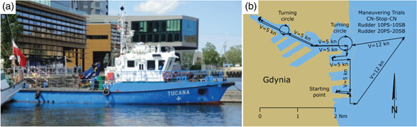
Increasing traffic of large-tonnage ships in the Bay of Gdansk requires studies to assess the positioning accuracy of GNSS systems used in navigation in the vicinity of ports. Modern GNSS receivers increase their positioning accuracy with propagation corrections broadcast by DGPS reference stations on Medium Frequency (MF) radio waves and large-area corrections, in European waters, transmitted by the EGNOS system by geostationary satellites. Positioning accuracy studies conducted so far for GNSS systems in the Bay of Gdansk have been conducted during stationary measurements (Sniegocki et al., Reference Sniegocki, Specht and Specht2014). For a vessel in motion and one manoeuvring on an approach to a port or within it, it is important to know the dynamic positioning error. To this end, measurements were conducted in a moving ship performing typical manoeuvres. However, there are no criteria for determination of a dynamic positioning error, but the International Maritime Organization (IMO) has developed standard manoeuvres used to determine the manoeuvring capability of ships to verify whether they comply with the valid standards. These include attempts at zigzagging, circling and stopping a ship. IMO standards (IMO, 2002) were employed to plan manoeuvres performed during dynamic measurements. Additionally, a simulated turn of a large ship on a turning circle within the Gdynia port was planned as well as manoeuvres of approaching and leaving the wharf. The planned route is shown in Figure 1(b).

Figure 1. The buoy tender “Tucana” (a) and the planned study route (b).
2.2. Measurements
The satellite measurements for this study were performed as part of periodical tests of the DGPS and EGNOS systems. The buoy tender Tucana, owned by the Maritime Office in Gdynia, was used for the purpose (Figure 1(a)). The measurements were conducted in the basin and at the roadstead of the Port of Gdynia. Details of the course, velocity and manoeuvres of the vessel are shown in Figure 1(b).
A ship fix platform on which the measuring equipment was installed was prepared before the tests. Four GNSS receivers were placed on it: two Trimble R10s (marked R1 and R2), a Trimble GA530 (S1) and a Simrad MXB5 (S2). The receivers were used to conduct satellite measurements with three types of corrections: DGPS (S2), EGNOS (S1) and Real-Time Kinematic (RTK) (R1 and R2). The platform was fixed on the upper deck of the Tucana in the structural axis of the vessel (Figure 2).

Figure 2. Position of the GNSS antennae on the Tucana.
A local (ship fix) system of coordinates was established for the study with the beginning at the central point of the first receiver's (R1) upper cover. It was assumed in this system of coordinates that the horizontal axis X was directed at the centre of the upper cover of receiver R2, the vertical axis Z (height) was perpendicular to the upper cover of receiver R1 and axis Y completed the counter-clockwise system of Cartesian coordinates (Figure 2). In the next preparatory stage to the main part of the measurements, the geometric mutual relationships between the receivers were determined. The tachymetric technique was employed for precision positioning of the measuring equipment. To this end, an electro-optical Leica TPS 1103 range finder was used to determine the coordinates within the local system of coordinates. The GNSS receivers had the following x, y, z coordinates in the local system: R1(0·000, 0·000, 0·000) (m), S1(0·372, 0·003, −0·115) (m), S2(0·746, 0·003, −0·105) (m), R2(0·000, 1·116, −0·003) (m). Subsequently, they were used to determine direction vectors vdS1 and vdS2 of the tested receivers S1 and S2 relative to the reference receiver R1:
 $$\hbox{vd}_{{\rm S1}}^{\rm T} = \left[ {\matrix{ {0\cdot 372} \cr {0\cdot 003} \cr {-0\cdot 115} \cr } } \right]$$
 $$\hbox{vd}_{{\rm S2}}^{\rm T} = \left[ {\matrix{ {0\cdot 746} \cr {0\cdot 003} \cr {-0\cdot 105} \cr } } \right]$$
When the measuring equipment was prepared and calibrated, the maritime dynamic measurements were started. They were conducted around noon on 20 June 2017. The weather conditions on the day were south-west wind force 4–5 (Beaufort scale), turning to north-west force 5–6, locally up to force 7, sea state in the Bay of Gdansk was 2–3 (Douglas sea scale), air temperature was around 16°C and visibility was good (IMGW-PIB, 2017). The tests were carried out in typical good weather conditions.
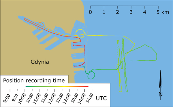
The Tucana unmoored from President's Wharf in Gdynia at about 10:00 and entered the roadstead of the Port of Gdynia. After the data registration was started, the ship headed towards the fairway leading to the main entrance to the Port of Gdynia. After attempts at zigzagging, circulation in the opposite direction and stopping, the Tucana entered the outer port in Gdynia by the main entrance and made a simulated large ship turn on the turning circle. Subsequently it sailed on to the port basins at a speed of approximately 10 knots, doing another simulated large ship turn on the turning circle in the Eighth Container Basin. Following the circulation of the port, the vessel continued its movement to the western end of the basin and approached the First Hel Wharf where container ships are moored. After the ship left the wharf, it started its return journey to the President's Wharf with a simulated approach to the Danish Wharf in the Third Coal Basin. After this manoeuvre, the Tucana sailed on to its final position at the President's Wharf, where it moored at around 14:00. The trajectory of the Tucana during the measurements is shown in Figure 3.

Figure 3. Ship's trajectory recorded during measurements.
The major part of the measurements involved recording the position coordinates obtained by GNSS receivers. Two of them (R1 and R2) were reference receivers, that is, they provided information which enabled determination of the positioning errors for the other two receivers (S1 and S2). For this purpose, RTK corrections of the commercial GNSS geodetic network VRSNet.pl were used, ensuring an accuracy of 2–3 cm (Earth fix system). Considering the expected accuracy of the receivers S1 and S2 (0·5–3 m), this range of values was adopted as sufficient for this study. All the receivers operated at a frequency of 1 Hz. Data from the S1 and S2 receivers involved recording NMEA GGA messages. Furthermore, during RTK measurements, reference receivers R1 and R2 performed real-time conversion of the Earth-Centred-Earth-Fixed (ECEF) coordinates into flat coordinates in the Gauss-Kruger projection. Since two types of coordinates were recorded in S1 and S2 (B, L, h) and R1 and R2 (xPL-2000, yPL-2000, H) receivers, it was necessary to reduce them to a uniform reference system (like in the reference receivers).
Coordinates in the local (ship fix) system of reference can be presented as vectors which determine the position of R2, S1 and S2 receivers relative to the R1 receiver. At a later stage, the vectors will help to determine the reference values for momentary coordinates of the tested receivers S1 and S2. Additionally, when the highly accurate coordinates are known (millimetre errors in tachymetric measurements), the real (nominal) values of coordinate increments between reference receivers R1 and R2 will also be known. Considering that the receivers also determine their coordinates in real time (with a much smaller error of 2–3 cm in the RTK method), this information can be used to calculate coordinate corrections.
The spatial relationships between the reference receivers were as follows: the horizontal distance between them was d = 1·116 m, and the difference of height dH = −0·003 m. Considering a high accuracy of the tachymetric technique, these values were taken as real. This data and the recorded coordinates of the receivers R1( xR1, yR1, HR1) and R2( xR2, yR2, HR2) were used to determine the random errors in each measurement epoch:
 $$\hbox{md}=\vert \hbox{R}_1 \hbox{R}_2\vert -\hbox{d}$$
 $$\hbox{mH}=(\hbox{H}_{\rm R2} -\hbox{H}_{\rm R1})-\hbox{dH}$$
where md is a momentary error of distance between receivers R1 and R2,  $\vert \hbox{R}_{1} \hbox{R}_{2}\vert =\sqrt{\lpar \hbox{x}_{\rm R2} -\hbox{x}_{\rm R1}\rpar ^{2}+\lpar \hbox{y}_{\rm R2} -\hbox{y}_{\rm R1}\rpar ^{2}}$ is the distance between receivers R1 and R2, determined by a GNSS measurement of coordinates of receivers R1( xR1, yR1) and R2( xR2, yR2), d is the actual (real) distance between receivers R1 and R2, mH is the momentary error of difference of height between receivers R1 and R2 and dH is the actual difference of height between receivers R1 and R2.
The reference receivers calculated momentary errors of horizontal coordinates: mXYR1 and mXYR2 and of normal height: mHR1 and mHR2 at every measurement. They made it possible to determine corrections for the measured coordinates:
 $$\Delta \hbox{d}_{{\rm R1}} = \left( {\displaystyle{{\hbox{m}_{{\rm XYR1}}} \over {\hbox{m}_{{\rm XYR1}} + \hbox{m}_{{\rm XYR2}}}}} \right)\hbox{md}$$
 $$\Delta \hbox{d}_{{\rm R2}} = \left( {\displaystyle{{\hbox{m}_{{\rm XYR2}}} \over {\hbox{m}_{{\rm XYR1}} + \hbox{m}_{{\rm XYR2}}}}} \right)\hbox{md}$$
 $$\Delta \hbox{H}_{{\rm R1}} = \left( {\displaystyle{{\hbox{m}_{{\rm HR1}}} \over {\hbox{m}_{{\rm HR1}} + \hbox{m}_{{\rm HR2}}}}} \right)\hbox{mH}$$
 $$\Delta \hbox{H}_{{\rm R2}} = \left( {\displaystyle{{\hbox{m}_{{\rm HR2}}} \over {\hbox{m}_{{\rm HR1}} + \hbox{m}_{{\rm HR2}}}}} \right)\hbox{mH}$$
where ΔdR1 and ΔdR2 are corrections for the calculated horizontal distance between reference receivers for R1 and R2, respectively and ΔHR1 and ΔHR2 are corrections for the calculated difference of normal heights between reference receivers for R1 and R2, respectively.
These corrections were used to calculate corrected coordinates of reference receivers:
 $$\hbox{x}_{{\rm R1}}^* = \hbox{x}_{{\rm R1}} + \Delta \hbox{d}_{{\rm R1}}\displaystyle{{\hbox{x}_{{\rm R2}}-\hbox{x}_{{\rm R1}}} \over {\vert \hbox{R}_1\hbox{R}_2\vert }}$$
 $$\hbox{x}_{{\rm R2}}^* = \hbox{x}_{{\rm R2}}-\Delta \hbox{d}_{{\rm R2}}\displaystyle{{\hbox{x}_{{\rm R2}}-\hbox{x}_{{\rm R1}}} \over {\vert \hbox{R}_1\hbox{R}_2\vert }}$$
 $$\hbox{y}_{{\rm R1}}^* = \hbox{y}_{{\rm R1}} + \Delta \hbox{d}_{{\rm R1}}\displaystyle{{\hbox{y}_{{\rm R2}}-\hbox{y}_{{\rm R1}}} \over {\vert \hbox{R}_1\hbox{R}_2\vert }}$$
 $$\hbox{y}_{{\rm R2}}^* = \hbox{y}_{{\rm R2}}-\Delta \hbox{d}_{{\rm R2}}\displaystyle{{\hbox{y}_{{\rm R2}}-\hbox{y}_{{\rm R1}}} \over {\vert \hbox{R}_1\hbox{R}_2\vert }}$$
 $$\hbox{H}_{\rm R1}^\ast =\hbox{H}_{\rm R1} +\Delta \hbox{H}_{\rm R1}$$
 $$\hbox{H}_{\rm R2}^\ast =\hbox{H}_{\rm R2} +\Delta \hbox{H}_{\rm R2}$$
where  $\lpar \hbox{x}_{\rm R1}^{\ast} \comma \; \hbox{y}_{\rm R1}^{\ast} \comma \; \hbox{H}_{\rm R1}^{\ast}\rpar \comma \; \lpar \hbox{x}_{\rm R2}^{\ast} \comma \; \hbox{y}_{\rm R2}^{\ast} \comma \; \hbox{H}_{\rm R2}^{\ast}\rpar $ are corrected coordinates of receivers R1 and R2.
By applying corrections to the calculated coordinates, it was possible to obtain a nominal geometric configuration between the receivers. This additionally reduced the error arising from the applied RTK technique in each measurement epoch. Since they were positioned in the ship axis, the reference receivers enabled determination of the momentary course of the vessel Heading (HDG) based on their corrected horizontal coordinates  $\lpar \hbox{x}_{\rm R1}^{\ast} \comma \; \hbox{y}_{\rm R1}^{\ast}\rpar $ and $\lpar \hbox{x}_{\rm R2}^{\ast} \comma \; \hbox{y}_{\rm R2}^{\ast}\rpar $:
 $$\hbox{HDG} = \arctan \left( {\displaystyle{{\hbox{y}_{{\rm R2}}^* -\hbox{y}_{{\rm R1}}^* } \over {\hbox{x}_{{\rm R2}}^* -\hbox{x}_{{\rm R2}}^* }}} \right)$$
 With two vectors of coordinates of the reference receivers  $\lpar \hbox{x}_{\rm R1}^{\ast} \comma \; \hbox{y}_{\rm R1}^{\ast} \comma \; \hbox{H}_{\rm R1}^{\ast}\rpar $ and $\lpar \hbox{x}_{\rm R2}^{\ast} \comma \; \hbox{y}_{\rm R2}^{\ast} \comma \; \hbox{H}_{\rm R2}^{\ast}\rpar $, and with the current course of the vessel HDG and the mutual spatial configuration of the measurement platform, it was possible to calculate the momentary coordinates of the tested receivers S1 and S2:
 $$\hbox{x}_{\rm i} =\hbox{x}_{\rm R1}^\ast +\hbox{vd}_{\rm ix} \cdot \cos (\hbox{HDG})-\hbox{vd}_{\rm iy} \cdot \sin (\hbox{HDG})$$
 $$\hbox{y}_{\rm i} =\hbox{y}_{\rm R1}^\ast +\hbox{vd}_{\rm ix} \cdot \sin (\hbox{HDG})+\hbox{vd}_{\rm iy} \cdot \cos (\hbox{HDG})$$
 $$\hbox{H}_{\rm i} =\hbox{H}_{\rm R1}^\ast +\hbox{vd}_{\rm iH}$$
where i is number of the tested receiver (1 or 2), xi, yi and Hi are momentary coordinates of the tested receivers and vdix, vdiy and vdiH are coordinates of the direction vector of the i-th receiver in the local (ship) system of coordinates.
2.3. Results
In marine navigation, several measures of the accuracy of position determination are used. Specifications of a Position Navigation and Timing (PNT) system accuracy generally refer to one or more of the following definitions:
Predictable accuracy: The accuracy of a PNT system's position solution with respect to the charted solution. Both the position solution and the chart must be based upon the same geodetic datum.
Repeatable accuracy: The accuracy with which a user can return to a position whose coordinates have been measured at a previous time with the same PNT system.
Relative accuracy: The accuracy with which a user can measure position relative to that of another user of the same PNT system at the same time.
The most important of these is predictable accuracy. Hence, in this paper all analyses are reported to this value.
Calculations aimed at determination of the position errors by receivers S1 and S2 were started by comparing the measured coordinates with the reference coordinates (Equations (16)–(18)). The differences of plane coordinates (Delta Northing - ΔY, Delta Easting - ΔX) and the normal height (Delta Height - ΔH) were calculated for each measurement epoch. Subsequently, the known values of coordinate increments (ΔY, ΔX) were used to calculate the momentary error on a horizontal plane (Two-Dimensional (2D) distance) based on the Pythagorean theorem on the ratio of sides in a right-angled triangle. Furthermore, an error in the vertical plane (height) was a direct consequence of an increment of normal heights (ΔH).
Figure 4 presents the horizontal position error distributions of EGNOS and DGPS receivers determined relative to the reference values. The red and green circles on the figures show the probability of a horizontal error: 68·3% (Distance Root Mean Square (DRMS)) and 95·4% (2DRMS).
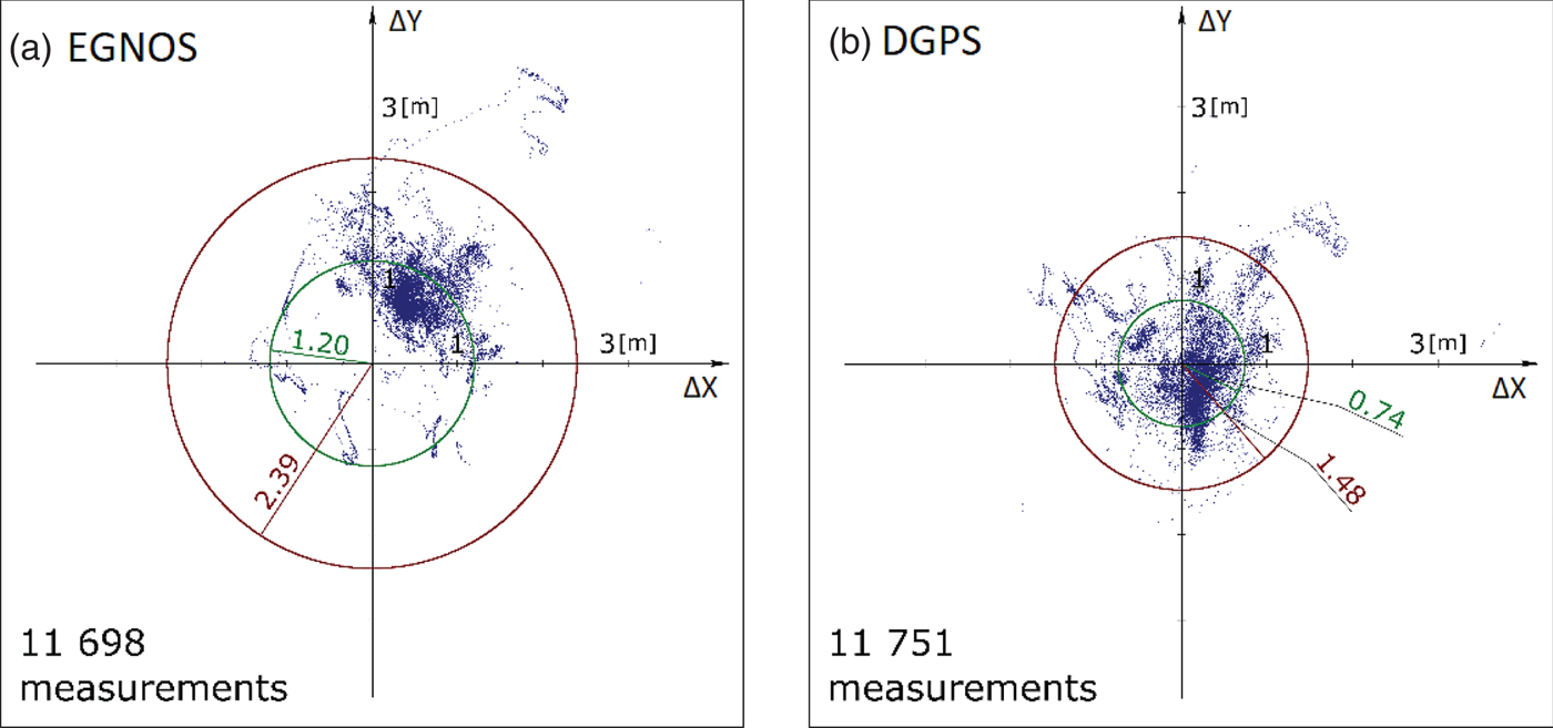
Figure 4. Horizontal position error distributions recorded by EGNOS (left) and DGPS (right) receivers.
Receiver S1 used EGNOS corrections during the maritime dynamic measurements. Registration of coordinates was continuous and there were no significant interruptions. A comparison of the coordinates determined in the study with the reference coordinates shows a distinct trend in distribution of horizontal coordinate errors. A large majority of them occurred in the north-eastern direction relative to the actual position of the receiver. The radius of the circle which determines the mean error of the horizontal position (DRMS) at the level of confidence of 1σ was 1·20 m (green in Figure 4(a)). Furthermore, the other of the measures under analysis (2DRMS) reached the level of 2·39 m (red in Figure 4(a)). This horizontal position error distribution is characterised by a relatively high precision with some outlying anomalies. The accuracy is much lower because of the permanent shift of errors by around 1 m relative to the actual position of the receiver.
The other receiver S2 using DGPS corrections recorded nearly an identical number of measurements as receiver S1 which used EGNOS corrections (Figure 4(b)). The data were registered successfully, with no adverse events (as with receiver S1). This horizontal position error distribution shows that the DGPS system is highly accurate and precise. Mean errors of horizontal position are nearly half those recorded in the EGNOS system and are: DRMS = 0·74 m (green circle in Figure 4(b)) and 2DRMS = 1·48 m (red circle in Figure 4(b)).
Errors in position coordinates of the tested receivers were assessed by means of the position accuracy measures, commonly used in navigation and geodesy, which are collectively presented in a tabular form (Table 1) (NovAtel Positioning Leadership, 2003; Van Diggelen, Reference Van Diggelen2007; Whelan and Taylor, Reference Whelan and Taylor2013).
Table 1. Position accuracy measures for GNSS receivers using DGPS and EGNOS corrections.
Table 1 shows that the DGPS system delivered better accuracy than the EGNOS system. One-dimensional measures (RMS) for both systems lie within a range between 0·5 and 1 m. However, the height errors (H) are greater than those for horizontal coordinates (x, y). For two-dimensional measures, they can be divided into three groups in terms of the probability of occurrence of a positioning error, which is, respectively: 50% (Circular Error Probable (CEP)), 68·3% (DRMS, R68) and 95·4% (2DRMS, R95). For the DGPS system, the measures of CEP, DRMS, R68 were a little over 0·5 m, whereas for the EGNOS system, they lay within a range of 1–1·2 m. Furthermore, measures in the horizontal plane where the probability of an error occurrence is increased (2DRMS, R95) were similar in the DGPS system and they did not exceed 1·5 m, whereas they differed more in the EGNOS system and they were: 2·39 m (2DRMS) and 1·79 m (R95). The analysis also took into consideration the Three-Dimensional (3D) position accuracy measures (Spherical Error Probable (SEP), DRMS, R68, R95). The SEP measure (p = 0·5) was 0·86 m for the DGPS system and 1·26 m for EGNOS. The next two pairs of measures (DRMS, R68) were greater than the previous ones by 25–30 cm at the 2σ level of confidence and they were approximately 1·1 m (DGPS) and 1·6 m (EGNOS). The highest values were calculated for the measures of R95(3D), which exceeded 2 m for both systems.
3. CONCLUSIONS
The aim of this study was to assess the accuracy of the DGPS and EGNOS systems during the manoeuvring of a vessel in the Bay of Gdansk. To this end, four-hours' worth of dynamic measurements were conducted, during which approximately 11,500 determinations of position coordinates were performed for each GNSS receiver. They were used as a basis for calculation of the position accuracy measures by the two systems.
An analysis of the study results showed that R95(2D) and R95(3D) measures in the DGPS system were 1·42 m and 2·07 m, respectively. These values were similar, but slightly worse than those obtained during the stationary measurements in 2014 (Sniegocki et al., Reference Sniegocki, Specht and Specht2014). However, it should be noted that the 2014 measurements were static and there was no need for continual determination of the reference coordinates in each measurement epoch (which could result in additional errors), as was the case in the dynamic study. A 2017 study showed that the DGPS system meets the accuracy requirements laid down in the standard issued by IALA (IALA, 2004). The R95(2D) measure is over seven times smaller than the acceptable value of 10 m in a horizontal plane (p = 0·95). Therefore, the Polish DGPS system can be used, for example, in the positioning of ships while entering a port, in coastal navigation, hydrography or in some geodetic applications.
The calculated accuracy of position coordinate determination shows that the DGPS system has slightly better accuracy characteristics than the EGNOS system. Smaller errors (on average 1·5 times) were achieved in all of the position accuracy measures. The measures of interest for the EGNOS system, R95(2D) and R95(3D), were as follows: 1·79 m and 2·80 m, which is nearly the same as in stationary measurements (Sniegocki et al., Reference Sniegocki, Specht and Specht2014). The accuracy of the open service in the EGNOS system should not be lower than 3 m in a horizontal plane and 4 m in a vertical plane (p = 0·95) (EC-DG Enterprise and Industry, 2017).
This study on DGPS and EGNOS systems in the Gulf of Gdansk has shown that in terms of the position accuracy, both systems meet the requirements of the IMO defined in Resolution A.1046(27) – Worldwide Radionavigation System (IMO, 2011). Its regulations include requirements for the following phases of marine navigation: harbour entrances, harbour approaches and coastal waters (minimum accuracy 10 m, p = 0·95), navigation in ocean waters (minimum accuracy 100 m, p = 0·95). It should be added that the tested systems do not meet a number of requirements related to other types of activities at sea, which are not related to the safety of navigation. These include, for example, resource exploration, engineering and construction. (Federal Radionavigation Plan (FRP), 2017). In addition, the EGNOS system does not meet the minimum positioning International Hydrographic Organization (IHO) Standards for Hydrographic Surveys, in a special category (IHO, 2008).


 Open access