2. Model-based architecture

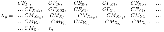
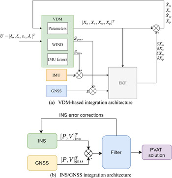
Figure 1 shows the model-based architecture investigated compared with a conventional INS/GNSS integration scheme which is more common in low-cost UAVs. The model-based architecture uses the dynamic model of a fixed-wing UAV as the main process model coupled with IMU and GNSS measurements using an extended Kalman filter (EKF). The architecture uses rotation rate and specific force measurements from the IMU as well as position measurements from the GNSS receiver in the fusion filter to estimate corrections to the navigation states. The control inputs from the autopilot system are used to propagate the navigation states. Mass and moment of inertia are assumed to be known and constant during the flight setup. The VDM requires a set of parameters $({X_P})$ used to derive the moments and forces acting on the aircraft, as can be seen in Figure 2. Pre-calibration of these parameters before a flight is possible but this can be time-consuming and usually requires expensive equipment.

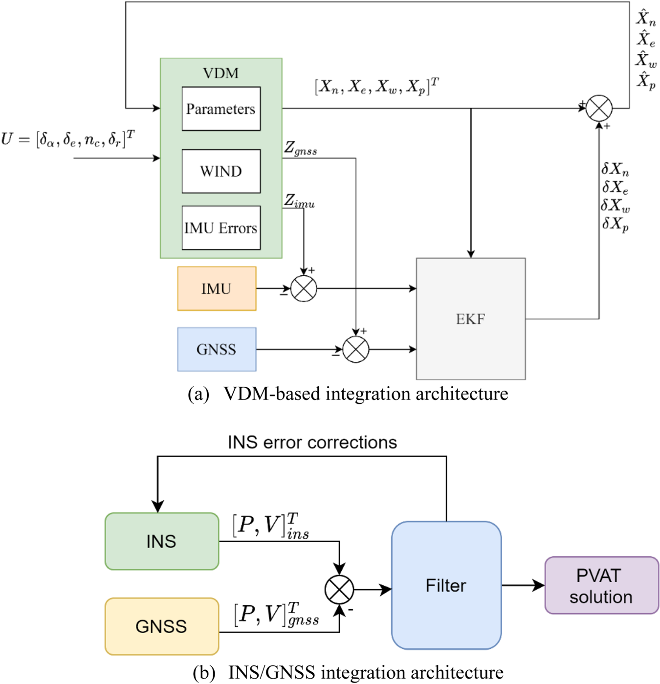
Figure 1. (a) VDM-based integration architecture, where ${\delta _\alpha },\; {\delta _e},\; {n_c},\; {\delta _r}$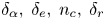 represent the aileron, elevator, propeller speed command and rudder deflection, respectively; ${Z_{gnss}}$, ${Z_{imu}}$ represent the GNSS and IMU measurement model; ${X_n},\; {X_e},\; {X_w},\; {X_p}$ represent the navigation states, IMU error states, wind error states and VDM parameter states, respectively. (b) INS/GNSS integration architecture, where PVAT represent the position, velocity, attitude and time solution; $[P,V]^{T}_{ins}$ represent the position and velocity solution from the INS and $[P,V]^{T}_{gnss}$ is output from the GNSS receiver

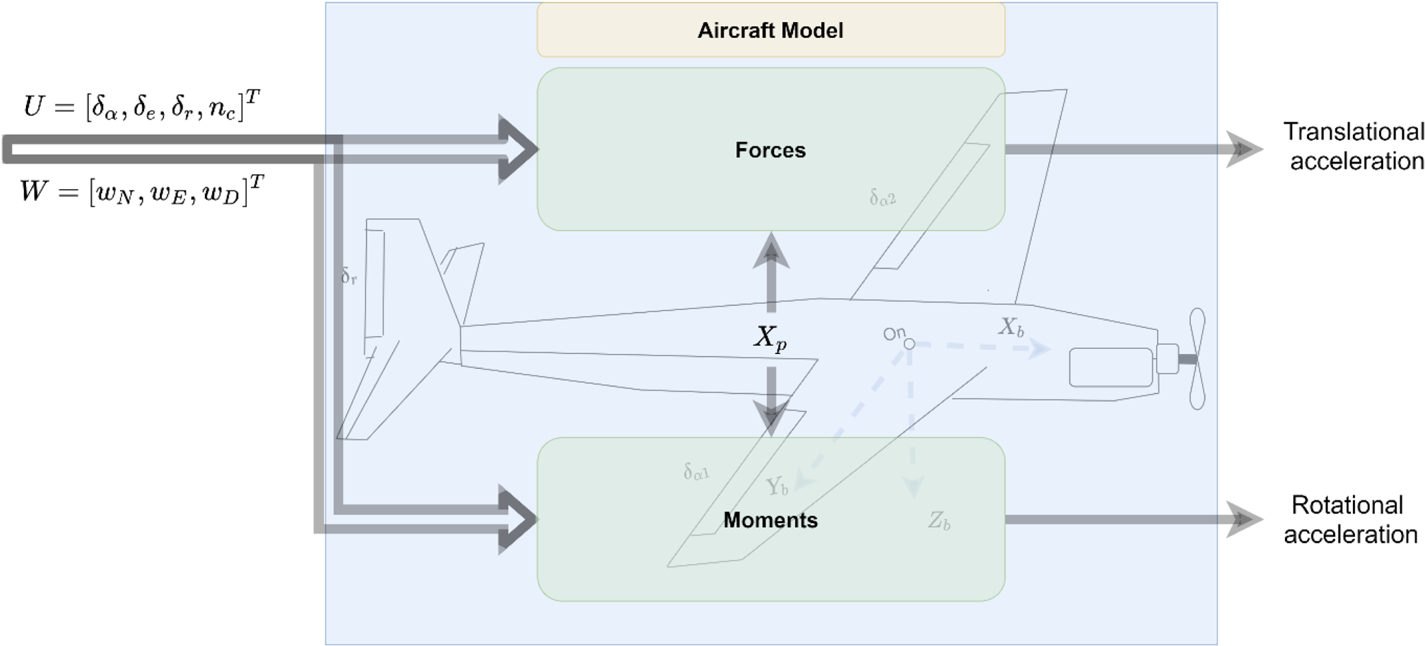
Figure 2. Diagram of VDM. It requires control inputs and wind velocity vector as inputs, which translate to translational and rotational accelerations that are integrated to propagate the navigation states

The VDM structure enables the inflight calibration of these parameters reducing the effort in obtaining accurate parameters. Figure 3 shows the coordinate frames considered in the investigation alongside the control surface deflections. Table 1 shows the formulation details for the airspeed, angle of attack $\mathrm{(\alpha )}$ and side-slip angle $\mathrm{(\beta )}$, respectively.

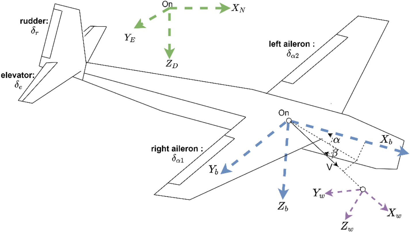
Figure 3. Coordinate frames used in the formulation of the equations of motion. ${[{X\; Y\; Z} ]_{[{b,w} ]}}$ represent the body frame (b) and wind frame (w) axes, respectively

Table 1. Airspeed, angle of attack and side-slip angle

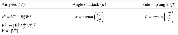
Note:$R_n^b$: local level (NED) to body rotation matrix; ${W^n}$: wind velocity vector in the NED frame.

3. Simulation setup and equations of motion

A Monte Carlo simulation study with 50 simulations is used to study the error characteristics of the architecture in Matlab. More details on the Monte Carlo simulation will be given in the next section.

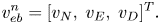
The VDM navigation states considered in the simulation are:

\[{X_n} = {[{r_{eb}^n,v_{eb}^n,{\phi_{nb}},\; \omega_{ib}^b,\; n} ]^T}.\]

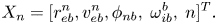
where $r_{eb}^n = {[{\mu \; \lambda \; {h_b}} ]^T}$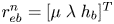 is the curvilinear position vector representing latitude, longitude and geodetic height, respectively. The velocity vector in the north-east-down (NED) frame is given by:

\[v_{eb}^n = {[{{v_N},\; {v_E},\; {v_D}} ]^T}.\]

The Euler angles, roll, pitch and yaw are given by:

\[{\phi _{nb}} = {[{\phi ,\theta ,\psi } ]^T}\]

and the rotation rate vector $\omega _{ib}^b = {[{{\omega_x},\; {\omega_y},\; {\omega_z}} ]^T}$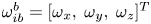represents the rotation around the roll, pitch and yaw axis. An arbitrary vector $V_{\alpha \beta }^\gamma$ represents a vector in the $\beta$ frame (object frame) with respect to the $\alpha$ frame (reference frame) resolved into the $\gamma$ frame (resolving frame). n is the propeller speed implemented as a first-order process. The rigid body equations of motion are given by:

(1)\begin{align}\dot{r}_{eb}^n &= {\left[ {\begin{matrix} {\dfrac{{v_{eb,N}^n}}{{{R_M} + h}}},&{\dfrac{{v_{eb,E}^n}}{{({{R_P} + h} )\cos\mu }}},&{ - v_{eb,D}^n} \end{matrix}} \right]^T} \end{align}

(2)\begin{align}\dot{v}_{eb}^n &= R_b^nf_{ib}^b + {g^n} - ({2\mathrm{\Omega }_{ie}^n + \mathrm{\Omega }_{en}^n} )v_{eb}^n\end{align}

(3)\begin{align}\dot{\phi } &= {R_\phi }({\omega_{ib}^b - R_n^b({\omega_{ie}^n + \omega_{en}^n} )} )\notag\\ R_{\phi} & = \left[ {\begin{matrix} {1 }&{ \tan\theta\sin\phi}&{ \tan\theta\cos\phi}\\ {0 }&{\cos\phi}&{- \sin\phi}\\ {0 }&{ \dfrac{\sin\phi}{\cos\theta }}&{\dfrac{\cos\phi}{\cos\theta}} \end{matrix}}\right]\end{align}

(4)\begin{align}\dot{\omega }_{ib}^b &= {({{I^b}} )^{ - 1}}({{M_b} - \mathrm{\Omega }_{ib}^b({{I^b}\omega_{ib}^b} )} )\end{align}

(5)\begin{align}\dot{n} &= \frac{{({ - n + {n_c}} )}}{{{\tau _n}}}\end{align}

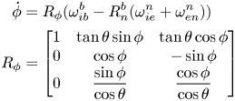
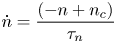
where ${g^n}$ is the gravity vector in the local NED frame, $I^b$ is the mass moment of inertia matrix, ${n_c}$ and ${\tau _n}$ represent the commanded propeller speed and time constant, respectively. The meridian $({R_M})$ and prime vertical $({R_P})$ radius of curvature are given by:

(6)\begin{equation}{R_M} = \frac{{{R_0}({1 - {e^2}} )}}{{{{({1 - {e^2}{{\sin }^2}(\mu )} )}^{3/2}}}}\ \textrm{and}\ {R_P} = \frac{{{R_0}}}{{{{({1 - {e^2}{{\sin }^2}(\mu )} )}^{1/2}}}}\end{equation}

where ${R_0}$ and e represent the semimajor axis and eccentricity, respectively. The specific force vector in the body frame $(f_{ib}^b)$ is given by:

(7)\begin{align} f_{ib}^b & =\dfrac{1}{m}\left( {R_w^b\left[ {\begin{matrix} {F_X^w}\\ {F_Y^w}\\ {F_Z^w} \end{matrix}} \right] + \left[ {\begin{matrix} {{F_T}}\\ 0\\ 0 \end{matrix}} \right]} \right)\notag\\ R_w^b & = \left[ {\begin{matrix} {\cos\alpha \cos\beta }&{ - \cos\alpha \sin\beta }&{ - \sin\alpha }\\ {\sin\beta }&{\cos\beta }&0\\ {\cos\beta \sin\alpha }&{ - \sin\alpha \sin\beta }&{\cos\alpha } \end{matrix}} \right] \end{align}

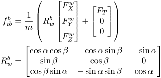
where $F_X^w,\; F_Y^w,\; F_Z^w$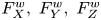 represent drag force, lateral force and lift force, respectively. ${F_T}$ is the thrust force and $R_w^b$ is the transformation matrix from the wind frame to the body frame. The moment term $({M_b})$ in the body frame is given by:-

(8)\begin{equation}{M_b} = {[{{M_X},{M_Y},{M_Z}} ]^T}\end{equation}

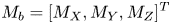
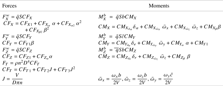
where ${M_X},\; {M_Y},\; {M_Z}$ represent the roll, pitch and yaw moments, respectively. Table 2 further represents the forces and moments acting on the aircraft using the VDM parameters. The actual values for the VDM parameters used in this work can be found in Ducard (Reference Ducard2007).

Table 2. Forces and moments acting on the aircraft

Note: $D\; :$ propeller diameter; $b\; :$ wingspan; $\rho \; \; :\;$ air density; $\bar{c}$: mean aerodynamic chord.

The aerodynamic and propulsion model presented in Table 2 describing the forces and moments acting on the aircraft can be found in Ducard (Reference Ducard2007) and Khaghani and Skaloud (Reference Khaghani and Skaloud2016).

4. Fusion filter and implementation

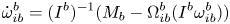
An EKF is used in the fusion of GNSS and IMU measurements with the VDM. Navigation states ${X_n}$ are propagated using the presented equations of motion. IMU errors $({X_e})$, wind velocity states $({X_w})$ and VDM parameters $({X_p})$ are propagated using a random walk process (Mwenegoha et al., Reference Mwenegoha, Moore, Pinchin and Jabbal2019). These states are given by:

(9)\begin{align}{X_e} &= {[{{b_{{a_1}}},{b_{{a_2}}},{b_{{a_3}}},{b_{{g_1}}},{b_{{g_2}}},{b_{{g_3}}}\; } ]^T}\end{align}

(10)\begin{align}{X_w} &= {[{{w_N},{w_E},{w_D}} ]^T}\end{align}

(11)\begin{align}{X_p} &= \left[ \begin{array}{@{}llllll@{}} {C{F_{{T_1}}},}&{C{F_{{T_2}}},}&{C{F_{{T_3}}},}&{C{F_{X1}},}&{C{F_{X\alpha }},}& \ldots \\ { \ldots C{F_{X\alpha 2}},}&{C{F_{X\beta 2}},}&{C{F_{Z1}},}&{C{F_{{Z_\alpha }}},}&{C{F_{Y1}},}& \ldots \\ { \ldots C{M_{{X_{{\delta_\alpha }}}}},}&{\; C{M_{{X_\beta }}},}&{\; \; \; C{M_{{X_{{{\bar{\omega }}_x}}}}},}&{\; \; \; C{M_{{X_{{{\bar{\omega }}_z}}}}},}&{C{M_{Y1}},}& \ldots \\ { \ldots C{M_{{Y_\alpha }}},}&{\; \; C{M_{{Y_{{\delta_e}}}}},}&{C{M_{{Y_{{{\bar{\omega }}_y}}}}},}&{\; \; C{M_{{Z_{{\delta_r}}}}},}&{\; C{M_{{Z_{{{\bar{\omega }}_z}}}}},}& \ldots \\ { \ldots C{M_{{Z_\beta }}},}&{{\tau_n}}&{}&{}&{}&{} \end{array} \right]\end{align}

The general form of the random walk process model for the IMU error states, wind velocity states and VDM parameters used in the navigation system is given by:

(12)\begin{equation}{\dot{X}_{[{e,w,p} ]}} = {G_{[{e,w,p} ]}}{W_{[{e,w,p} ]}}\end{equation}

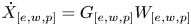
where ${G_{[{e,w,p} ]}}$ is the noise shaping matrix for the IMU error states, wind velocity states and VDM parameters, respectively. ${W_{[{e,w,p} ]}}$ is the driving noise vector for the IMU error states, wind velocity states and VDM parameters, respectively.

In the simulator, the IMU errors and wind model follow a first-order Gauss-Markov process, and their parameters are unknown to the filter while the VDM parameters were fixed. The first-order Gauss-Markov wind model used had a constant component with a magnitude of 3⋅8 m/s, a correlation time of 200 s, and a process uncertainty of 0⋅1 m/s. Generally, a first-order Gauss-Markov process $({X_{gm}})$ can be represented as:

(13)\begin{equation}{\dot{X}_{gm}} ={-} {\beta _{gm}}{X_{gm}} + {n_{gm}}\end{equation}

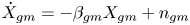
where ${\beta _{gm}}$ is the inverse of the correlation time and ${n_{gm}}$ is the driving noise.

The overall state vector is given by:

(14)\begin{equation}x = {[{{X_n},{X_e},{X_w},{X_p}\; } ]^T}\end{equation}

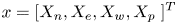
The measurement vector consists of IMU $(\tilde{f}_{ib}^b,\; \tilde{\omega }_{ib}^b)$ and GNSS $(\tilde{r}_{eb}^n)$ measurements.

(15)\begin{equation}Z = {[{{Z_{\textrm{IMU}}},{Z_{\textrm{GNSS}}}} ]^T}\end{equation}

where each measurement $(Z)$ is given by a measurement function $h$:

(16)\begin{equation}{Z_k} = h[{{x_k},\; {u_k}} ]+ {r_k}\end{equation}

where ${x_k}$ is the predicted state vector at the current time index k, ${u_k}$ is the known control input vector from the autopilot system and ${r_k}$ is the measurement noise where the expectation operator on the white sequence vector and its transpose is given by:

\[E[{{r_k}r_k^T} ]= {R_k}.\]

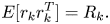
where ${R_k}$ is the measurement covariance. Therefore, the observation model for the IMU is given by:

(17)\begin{equation}{Z_{\textrm{IMU}}} = \left[ {\begin{array}{*{20}{c}} {f_{ib}^b + {X_e}({[{1\; 2\; 3} ]} )}\\ {\omega_{ib}^b + {X_e}({[{4\; 5\; 6} ]} )} \end{array}} \right] + {w_i}\end{equation}

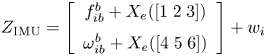
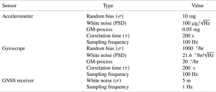
where the IMU measurement covariance $({R_{{i_k}}} = E[{w_{{i_k}}}w_{{i_k}}^T])$ is obtained from the simulated error characteristics presented in Table 4. The observation model for the GNSS measurements is given by:

(18)\begin{equation}{Z_{\textrm{GNSS}}} = {\left[ {\begin{array}{*{20}{c}} \mu \\ \lambda \\ h \end{array}} \right]} + {w_g}\end{equation}

where the GNSS measurement covariance $({R_{gk}} = \; E[{w_{gk}}w_{gk}^T])$ is obtained from simulated GNSS receiver error with minor scaling. The filter utilises the linearised version of the process model $(F = (\partial \dot{x}/\partial x))$ and observation model $(H = (\partial Z/\partial x)\; )$ on the prediction and update of the state vector and the covariance matrix. The observation matrix H is given by:

(19)\begin{align} H & =\dfrac{{\partial Z}}{{\partial x}} = \dfrac{{\partial {{[{{Z_{imu}}\; \; {Z_{gnss}}} ]}^T}}}{{\partial [{{X_n}\; {X_e}\; {X_w}\; {X_p}} ]}}\notag\\ & =\left[ {\begin{array}{*{20}{c}} {{H_{imu,n}}}\\ {{H_{gnss,n}}} \end{array}\; \begin{array}{*{20}{c}} {{H_{imu,e}}}\\ {{H_{gnss,e}}} \end{array}\; \begin{array}{*{20}{c}} {{H_{imu,w}}}\\ {{H_{gnss,w}}} \end{array}\; \begin{array}{*{20}{c}} {{H_{imu,p}}}\\ {{H_{gnss,p}}} \end{array}\; } \right] \end{align}

The EKF propagation and update steps are summarised in Table 3. Table 4 presents the stochastic properties of the sensors used in the simulation.

Table 3. EKF propagation and update

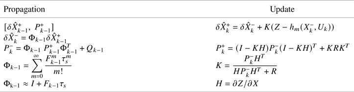
Table 4. Stochastic properties of the IMU and GNSS receiver

The trajectory used in the simulation is presented in Figure 4. The presented equations of motion, aerodynamic and propulsion models are implemented in Matlab/Simulink to generate the trajectory. The trajectory partly captures what would be experienced in a typical mapping or surveying mission. GNSS outages are induced during certain segments of the trajectory where the aircraft experiences rapid dynamics in roll, pitch, yaw or a combination of them, i.e., during turns.

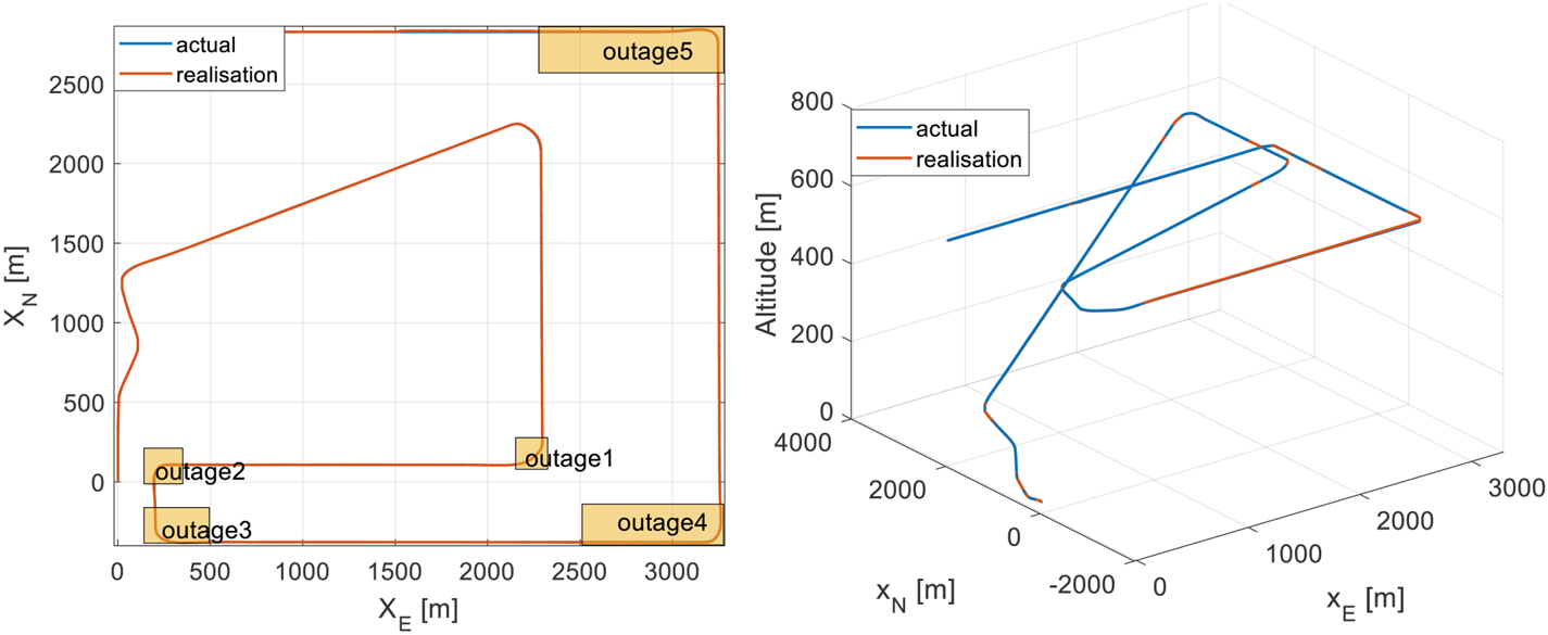
Figure 4. Trajectory used to study the error characteristics of a VDM/INS/GNSS architecture

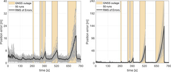
To evaluate the performance of the navigation system, a Monte Carlo simulation study has been performed with 50 runs. Errors are introduced to all the a priori information available such as the initial values for the navigation states, VDM parameters, statistics of the IMU and GNSS measurements. The trajectory and wind profile have been kept the same in each realisation. The error in observations, initialisation and VDM parameters is changed randomly in each run. VDM parameters are changed with a standard deviation of 10% of the initial values. The position errors for 50 Monte Carlo runs are presented in Figure 5.

Figure 5. Position errors for 50 Monte Carlo runs for the VDM/INS/GNSS (left) scheme and the INS/GNSS (right) integration architecture

A total of three simulations with the VDM architecture are performed with the given trajectory and three different autopilot settings. The autopilot limits the rotation rates to 15°/s, 30°/s and 60°/s, respectively. Figure 6 shows the GNSS outage and re-acquisition segments as well as the roll rates and roll angles achieved during the three runs. The outage period is set to 10 s, 20 s, 30 s, 60 s and 90 s, respectively during each simulation run, as seen in Figure 6.

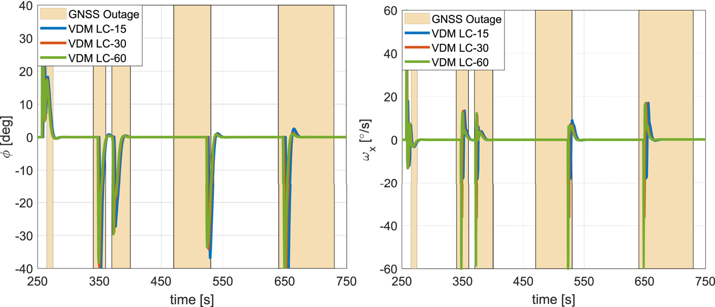
Figure 6. Dynamics in terms of roll angle (left) and roll rate (right) for the three simulation runs. VDM LC-15 represents the simulation run with 15°/s rate limit; VDM LC-30 represents the simulation run with 30°/s rate limit; VDM LC-60 represents the simulation run with 60°/s rate limit

5. Error characteristics results

The results from a Monte Carlo simulation study are presented in this section for the VDM approach and some comparison is made with an INS/GNSS approach. The initial 250 s of the flight are used for convergence and therefore removed from the discussion.

The position error is presented in Figure 7. For GNSS outages lasting up to 60 s, the results showed that the position error for the VDM approach with different rotation rate limits was similar. The position errors for the different rate cases reached only 8⋅494 m after 60 s of GNSS outage, well within the $2\sigma$ of the GNSS receiver modelled as opposed to 61 m for an INS/GNSS case. For GNSS outages lasting up to 90 s, the level of dynamics mostly around the roll axis seemed to influence position error, as shown in Figure 7 in the last outage phase. With a rate limit of 60°/s, the maximum position error was 16% greater than the position error observed with a rate limit of 15°/s and only 8% greater with a rate limit of 30°/s.

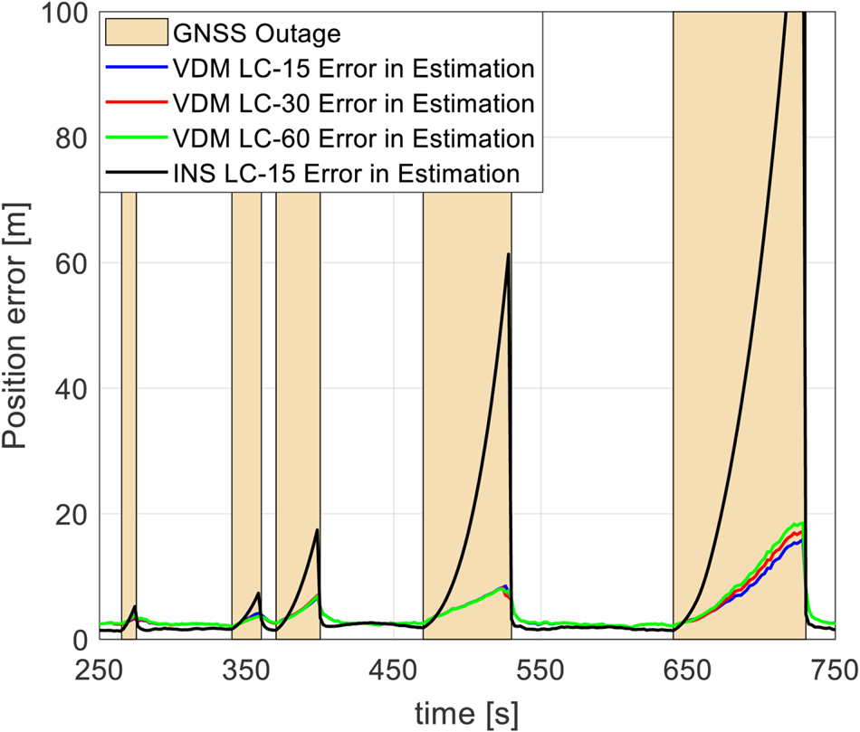
Figure 7. RMS of position error for VDM versus INS approach

With a GNSS outage lasting 90 s, the position error of the INS/GNSS approach with a rate limit of 15°/s was an order of magnitude higher than the VDM approach limited to 60°/s. The additional information from using the VDM reduced the rapid drift in the navigation solution, leading to superior performance by the VDM approach even with rapid roll dynamics.

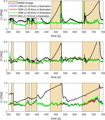
The root mean square (RMS) of the attitude errors is presented in Figure 8. For the VDM approach with different rotation rate limits, the overall roll and pitch angle errors during all periods of GNSS outage did not significantly change, excluding sections with rapid roll dynamics owing to the use of the VDM. However, yaw angle error seemed to increase gradually during an outage period, especially with some channel dynamics during the outage. Yaw angle error was found to increase, reaching a maximum value of 0⋅53 degrees, 0⋅55 degrees, 0⋅68 degrees and 0⋅8344 degrees during GNSS outages lasting 10 s, 20 s, 30 s and 90 s, respectively. The GNSS outage period lasting 60 s (fourth outage) showed small growth in yaw error, reaching a maximum value of 0⋅5 degrees. During the fourth outage (470–530 s), the aircraft experienced large rotation rates only during the last phase of the outage. Therefore, between 470 s and 520 s, the aircraft was flying mostly straight and level, causing only slight growth in yaw angle error, as can be seen in Figure 8.

Figure 8. Attitude errors for VDM versus INS approach

During a turn, the maximum rotation rate achieved was found to influence roll angle errors the most and pitch angle errors to a lesser extent. With a rate limit of 15°/s, the roll angle error reached a maximum of 0⋅17 degrees (654 s), while for 30°/s it reached a maximum of 0⋅36 degrees (650 s) and reached a maximum of 0⋅46 degrees (648 s) with a rate limit of 60°/s. With the VDM approach, the roll angle error quickly recovered after short periods of rapid roll dynamics. The large increase in roll angle error during sections with large rotation rates occurred even with GNSS availability with the VDM approach, as shown in the interval between 250 s and 265 s. The large instantaneous error, correlated with the rotation rate, is mainly attributed to the remaining part of the initialisation errors, especially in the VDM parameters. The use of the VDM prevented further growth of the attitude errors following rapid dynamics even in periods of extended GNSS outage lasting 90 s. On the other hand, with an INS/GNSS approach, the attitude errors grew rapidly, with the maximum error observed being correlated with the length of the outage period.

The accelerometer bias estimation error is presented in Figure 9. After filter convergence, the accelerometer bias estimation errors remained bounded and did not grow during the GNSS outages. The simple random walk model used to estimate the accelerometer bias provided reasonable results enabling good navigation performance for a flight period lasting 780 s with short periods of GNSS outage in between. Large roll rotation rates during an outage period did not seem to influence the estimation performance of the accelerometer bias following the convergence of the filter.

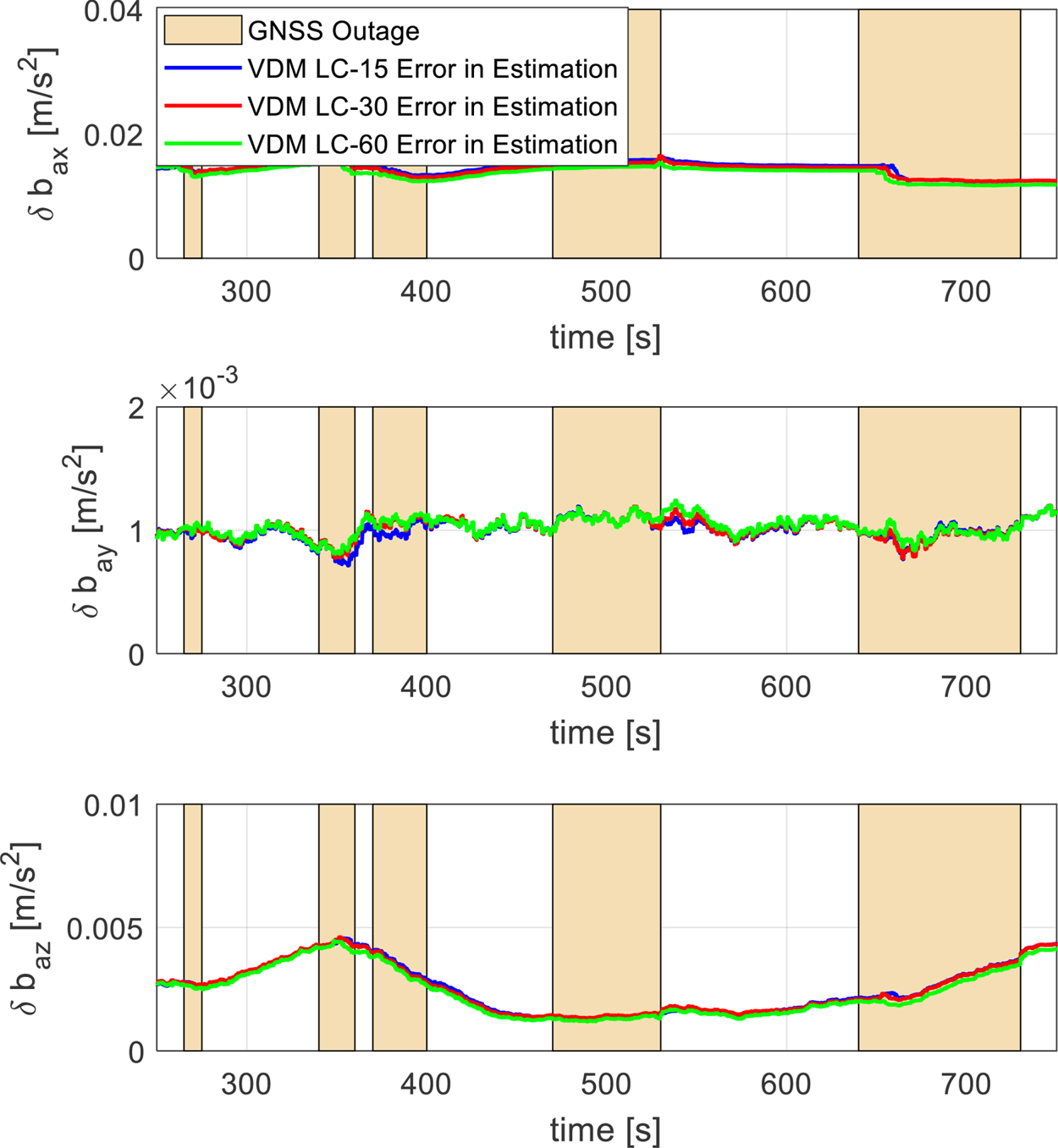
Figure 9. Accelerometer bias estimation errors for the VDM approach

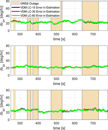
The gyroscope bias estimation error is presented in Figure 10. It was found that 98% of the initial turn-on gyroscope bias and bias variation was resolved well within 100 s of GNSS presence. And just like the accelerometer bias, GNSS outages of different lengths, 10 s, 20 s, 30 s, 60 s and 90 s, did not seem to influence the estimation error of the gyroscope bias owing to the use of the VDM and direct IMU measurements during the outage. Further, large roll rotation rates reaching 60°/s during the GNSS outages did not seem to influence the estimation of the gyroscope bias following the convergence of the filter.

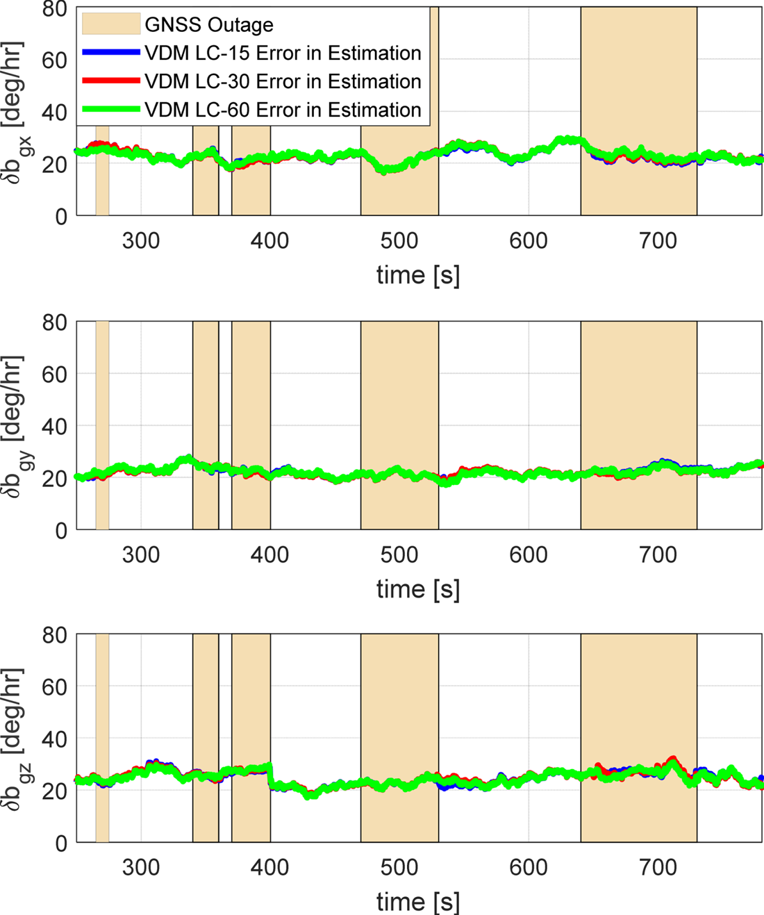
Figure 10. Gyroscope bias estimation errors for the VDM approach

The RMS of the mean error of 22 VDM parameters is presented in Figure 11. A GNSS outage alone lasting 10 s, 20 s, 30 s, 60 s or 90 s did not seem to influence the VDM parameter estimation error. However, turning during a GNSS outage actually led to improved observability of the VDM parameters, thanks to the availability of IMU measurements during this period. Further, a low roll rotation rate of 15°/s led to slightly better observability of VDM parameters as opposed to 60°/s, but the difference was just 0⋅5%.

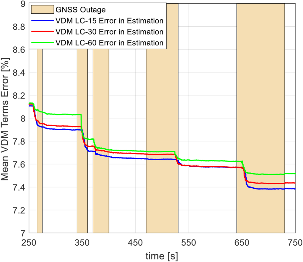
Figure 11. VDM parameters estimation error

Figure 12 shows the RMS of wind magnitude errors. The VDM approach provided the capability to estimate wind velocity, which in turn improved the navigation solution during GNSS outages as opposed to an INS/GNSS approach. It was found that GNSS outages lasting less than 60 s did not have a significant influence on the estimated wind magnitude error. With a GNSS outage lasting 90 s (fifth outage), the error in the estimated wind magnitude was found to grow gradually, reaching 0⋅2 m/s at the end of the fifth outage. The level of dynamics, especially in the roll axis, seemed not to influence the growth of wind magnitude error significantly.

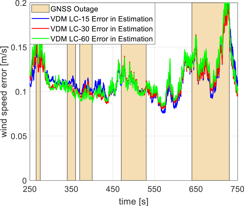
Figure 12. Wind speed error for VDM