

1. INTRODUCTION
The positioning performance of Global Navigation Satellite Systems (GNSS) in dense urban areas is poor because buildings block, reflect and diffract the signals. Many applications would benefit from better positioning in cities. Examples include vehicle lane detection for Intelligent Transportation Systems (ITS), location-based advertising, augmented-reality, and step-by-step guidance for the visually impaired and for tourists.
Buildings and other obstacles degrade GNSS positioning in three ways. Firstly, where signals are completely blocked, they are simply unavailable for positioning, degrading the signal geometry. Secondly, where the direct signal is blocked (or severely attenuated), but the signal is received via a (much stronger) reflected path, this is known as Non-Line-Of-Sight (NLOS) reception. NLOS signals exhibit positive ranging errors corresponding to the path delay (the difference between the reflected and direct paths). These are typically a few tens of metres in dense urban areas, but can be much larger if a signal is reflected by a distant building. Thirdly, where both direct Line-Of-Sight (LOS) and reflected signals are received, multipath interference occurs. This can lead to both positive and negative ranging errors, the magnitude of which depends on the signal and receiver designs. NLOS reception and multipath interference are often grouped together and referred to simply as “multipath”. However, to do so is highly misleading as the two phenomena have different characteristics and can require different mitigation techniques (Groves, Reference Groves2013b).
There are many different approaches to multipath and NLOS mitigation (Groves, Reference Groves2013a). Receiver-based signal processing techniques dominate a lot of the literature. However, because they work by separating out the direct and reflected signals within the receiver, they can only be used to mitigate multipath; they have no effect on NLOS reception at all. A good GNSS antenna is more sensitive to Right-Hand Circularly Polarised (RHCP) signals than to Left-Hand Circularly Polarised (LHCP) signals. As direct LOS signals are RHCP while most reflected signals are LHCP or mixed polarisation, this reduces errors due to multipath inference. It also enables most NLOS signals to be detected from the Signal to Noise Ratio (SNR) measurements and eliminated from the position calculation. However, cheaper antennae offer less polarisation discrimination and smartphone antennae none at all.
Consistency checking is based on the principle that measurements from “clean” direct LOS signals produce a more consistent navigation solution than those from NLOS and severely multipath-contaminated signals. Conventional sequential testing approaches work where the number of good measurements greatly exceeds the number of outliers. However, it works poorly in dense urban areas where lots of signals are affected by NLOS reception and multipath interference. Consistency checking using subset comparison is more robust under these conditions, but still needs a minimum number of good signals to work (Groves and Jiang, Reference Groves and Jiang2013).
Terrain height data is useful for outdoor positioning of both vehicles and pedestrians, who can be assumed to be a fixed height above the terrain. This can be used to generate a virtual ranging measurement that constrains the position solution (Amt and Raquet, Reference Amt and Raquet2006). One might expect this to only improve vertical position. However, where the signal geometry is poor, it also improves the horizontal position. In dense urban areas, this terrain height aiding improves the horizontal position accuracy by almost a factor of two (Adjrad and Groves, Reference Adjrad and Groves2017).
The increasing availability of Three-Dimensional (3D) mapping provides an opportunity to improve GNSS positioning in dense urban areas. 3D models of buildings can be used to predict which signals are blocked and which are directly visible at any location (Bradbury et al., Reference Bradbury, Ziebart, Cross, Boulton and Read2007; Suh and Shibasaki, Reference Suh and Shibasaki2007). This can be computationally intensive. However, the real-time computational load can be reduced dramatically by using building boundaries (Wang et al, Reference Wang, Groves and Ziebart2012). These describe the minimum elevation above which satellite signals can be received at a series of azimuths and are precomputed for each candidate position. A signal can then be classified as LOS or NLOS simply by comparing the satellite elevation with that of the building boundary at the corresponding azimuth.
Where the user position is already approximately known, it is straightforward to use a 3D city model to predict the NLOS signals and eliminate them from the position solution (Obst et al., Reference Obst, Bauer and Wanielik2012; Bourdeau and Sahmoudi, Reference Bourdeau and Sahmoudi2012; Peyraud et al., Reference Peyraud, Bétaille, Renault, Ortiz, Mougel, Meizel and Peyret2013). However, for most urban positioning applications there is significant position uncertainty. A search area containing the possible position solutions may be defined centred on the conventional GNSS position solution and the proportion of these candidate positions at which each signal is receivable via direct LOS may be predicted using the 3D mapping. This information can then be used to re-weight a least-squares position solution and aid consistency checking, improving the horizontal position accuracy by about 61% (Adjrad and Groves, Reference Adjrad and Groves2017). A more advanced approach is discussed under future work in Section 6.
Several research groups have taken the concept of 3D-Mapping-Aided (3DMA) GNSS ranging a step further by using a 3D city model to predict the path delay of the NLOS signals across an array of candidate positions (Suzuki and Kubo, Reference Suzuki and Kubo2013; Kumar and Petovello, Reference Kumar and Petovello2014; Hsu et al., Reference Hsu, Gu and Kamijo2016). A single-epoch positioning accuracy of 4 m has been reported (Hsu et al., Reference Hsu, Gu and Kamijo2016). Kbayer et al. (Reference Kbayer, Sahmoudi and Chaumette2015) used 3D mapping to predict lower and upper bounds for the biases due to NLOS reception and multipath interference, which were then used by a robust estimator to determine the position solution. However, unless the search area is small, these approaches are very computationally intensive as the path delay cannot easily be pre-computed. The urban trench approach presented in Betaille et al. (Reference Betaille, Peyret, Ortiz, Miquel and Fontenay2013) enables the path delays of NLOS signals to be computed very efficiently, but only if the building layout is highly symmetric.
Another way of using 3D city models to improve GNSS positioning in dense urban areas is shadow matching (Groves, Reference Groves2011). This determines position by comparing the measured signal availability and strength with predictions made using a 3D city model over a range of candidate positions. Since 2011, several research groups have experimentally demonstrated shadow matching and similar techniques, using both single and multiple epochs of GNSS data (Suzuki and Kubo, Reference Suzuki and Kubo2012; Wang et al., Reference Wang, Groves and Ziebart2013; Isaacs et al., Reference Isaacs, Irish, Quitin, Madhow and Hespanha2014; Wang et al., Reference Wang, Groves and Ziebart2015; Yozevitch and Ben-Moshe, Reference Yozevitch and Ben-Moshe2015). Across-street positions within a few metres have been achieved in environments where the error in the conventional GNSS position solution is tens of metres, enabling users to determine which side of the street they are on. This complements GNSS ranging, which is more accurate in the along-street direction in dense urban areas because more direct LOS signals are received along the street than across it. Shadow matching has also been demonstrated in real time on an Android smartphone.
Clearly, to get the best performance out of GNSS aided by 3D mapping, as much information as possible should be used. Thus, both pseudo-range and SNR measurements from a multi-constellation GNSS receiver should be used, together with both LOS/NLOS predictions and terrain height from 3D mapping. This concept is known as intelligent urban positioning (Groves et al., Reference Groves, Jiang, Wang and Ziebart2012).
This paper presents the first integration of GNSS shadow matching with 3DMA ranging, demonstrating its benefit. The shadow matching algorithm, based on the design presented in Wang et al. (Reference Wang, Groves and Ziebart2015), uses the SNR measurements to compute a position solution. The 3DMA ranging algorithm, described in Adjrad and Groves (Reference Adjrad and Groves2017), uses the pseudo-ranges to compute the position and incorporates the following techniques:
-
• Terrain height aiding;
-
• Weighting of GNSS ranging measurements according to the proportion of candidate positions at which each signal is predicted from 3D mapping to be direct LOS;
-
• Consistency checking by subset comparison.
Two new methods for integrating these two positioning techniques are presented and compared. Both use position-domain integration, where separate ranging and shadow matching position solutions are computed, then combined using direction-dependent weighting. The first approach weights the position solutions according to their covariances, but modifies the shadow matching covariance to account for multi-modality by computing the kurtosis. The second technique is based on the principle that shadow matching works better in the across-street direction and GNSS ranging in the along-street direction. It therefore uses the street direction and building height to street width ratio to determine a suitable weighting in each direction.
The different positioning and integration methods are compared using experimental data collected in London using a u-blox consumer-grade GNSS receiver and a Sony smartphone.
Section 2 summarises the algorithms for computing position from shadow matching and from 3DMA ranging. Section 3 describes the two algorithms for integrating shadow matching and ranging. Section 4 presents experimental test results. Finally, Section 5 summarises the conclusions and Section 6 discusses future work.
The algorithms presented here operate using a single epoch of GNSS measurements. This is suitable for location-based services, emergency caller location and low-update-rate tracking applications. For navigation and continuous tracking, the algorithms can be applied to successive epochs of data. However, as with conventional GNSS positioning, better performance can be obtained using a filtered approach. The aim of this paper is to demonstrate the benefit of integrating GNSS shadow matching with 3DMA ranging. Development of the best possible algorithms for shadow matching, 3DMA ranging and their integration is a subject for future research.
2. POSITIONING ALGORITHMS
GNSS position solutions are computed using both 3DMA ranging and shadow matching. Each is described in turn.
2.1 3D-Mapping-Aided Ranging
Figure 1 shows the 3DMA ranging algorithm, comprising the following six steps:
-
1. A search area is determined using the conventional GNSS position solution on the first iteration and the previous solution on subsequent iterations. Here, we used fixed-radius circles for simplicity. However, a search area based on an appropriate confidence interval would be more efficient.
-
2. Using building boundaries precomputed from the 3D city model (Wang et al., Reference Wang, Groves and Ziebart2012), the proportion of the search area within which each satellite is directly visible is computed, providing an estimate of the probability that the signal is direct LOS.
-
3. A consistency checking process is applied to the ranging measurements, making use of the direct LOS probabilities from the 3D mapping.
-
4. The set of signals resulting from the consistency checking process is subjected to a weighting strategy based on the previously determined LOS probabilities and carrier-power-to-noise-density ratio, C/N 0.
-
5. Digital Terrain Model (DTM) information is extracted from the 3D city model and a virtual range measurement is generated using the position at the centre of the search area.
-
6. Finally, a position solution is derived from the pseudo-ranges and virtual range measurement using least-squares estimation.
The algorithm is then iterated several times to improve the position solution, reducing the search radius each time from 100 m initially to 40 m on the final iteration. Full details are presented in Adjrad and Groves (Reference Adjrad and Groves2017).
2.2 Shadow Matching
Figure 2 shows the shadow matching algorithm, comprising the following five steps:
-
1. A circular search area of radius 40 m is defined with its centre at the 3DMA ranging position solution. This value was determined empirically. Within this search area, a grid of candidate positions at 1 m intervals is set up.
-
2. For each candidate position, the satellite visibility is predicted using the building boundaries precomputed from the 3D city model (Wang et al., Reference Wang, Groves and Ziebart2012). If the satellite elevation is above the building boundary at the relevant azimuth, the LOS probability predicted from the building boundary, p(LOS|BB), is set to 0·8. Otherwise, it is set to 0·2. These values allow for diffraction and 3D model errors and were determined empirically as described in Section 4.
-
3. The observed satellite visibility is determined from the GNSS receiver's C/N 0 or Signal to Noise Ratio (SNR) measurements. From these, a probability that each received signal is direct LOS, p(LOS|SNR = s) is estimated. The models used here are described in Section 4.
-
4. The next step is to score each candidate position according to the match between the predicted and measured satellite visibility. For a given satellite, the probability that the predicted and measured satellite visibility match, P m , is (Wang et al., Reference Wang, Groves and Ziebart2015)
(1)The overall score for each position, Λ S , is then the product of the individual satellite probabilities. $$P_m = 1 - p\lpar LOS \vert SNR = s \rpar - p (LOS \vert BB) + 2p \lpar LOS \vert SNR = s \rpar p(LOS\vert BB).$$
-
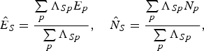
5. Finally, a position solution is determined based on a weighted average of the candidate positions. The weighting factor for each candidate is the normalised score, which is the relative probability of that candidate position. Thus, the position solution is
(2)where E p , N p and Λ Sp are the easting coordinate, northing coordinate and score of the p th candidate position.
$$\hat{E}_S = {\sum\limits_p \Lambda _{Sp} E_p \over \sum\limits_p \Lambda _{Sp}}, \quad \hat{N}_S = {\sum\limits_p \Lambda _{Sp} N_p \over \sum\limits_p \Lambda _{Sp}},$$

Full details of steps 1 to 4 are presented in Wang et al. (Reference Wang, Groves and Ziebart2015).
3. INTEGRATION ALGORITHMS
A position-domain approach to the integration of ranging-based GNSS positioning with GNSS shadow matching is implemented here. Thus, GNSS ranging and shadow-matching position solutions are computed separately and then integrated together. Where pseudo-range information from the user device is available, the conventional GNSS solution is enhanced using terrain height aiding, consistency checking and weighting of the pseudo-range measurements based on the average NLOS reception probability, as described in Adjrad and Groves (Reference Adjrad and Groves2017) and summarised in Section 2.1. This solution is referred to as the “3DMA GNSS ranging solution” in the remainder of this paper while “GNSS ranging solution” refers to either the conventional or the enhanced solutions.
An integrated position solution, x wav , may be obtained by computing the weighted average of the GNSS ranging and shadow matching position solutions. Thus,
 $${\bf x}_{wav} =\lpar {\bf W}_S +{\bf W}_R \rpar ^{-1} \lpar {\bf W}_S {\bf x}_S + {\bf W}_R {\bf x}_R \rpar ,$$
where x S and x R are respectively the shadow matching and GNSS ranging position solutions and W S and W R are the weight matrices for the respective solutions.
The challenge is then to determine suitable weighting matrices. Two different approaches are investigated here:
-
1. A covariance-based approach based on the computations of the ranging-based and shadow matching position error covariance matrices. The weighting matrices are then the inverses of the corresponding error covariance matrices.
-
2. A deterministic approach based on weighting the shadow matching and GNSS solution exploiting street azimuth information in a way such that shadow matching is given higher weights across-street and lower weights along-street (and vice-versa for the GNSS solution).
3.1 Covariance-based weighting approach
Weighting the GNSS ranging and shadow matching position solutions using the inverses of their respective error covariance matrices makes the implicit assumption that their error distributions are Gaussian. However, this is not the case in reality. For GNSS ranging, NLOS measurements have a skewed error distribution as the path delay is always positive, resulting in distortions to the resulting position error distribution. By down-weighting those measurements predicted more likely to be NLOS (Section 2.1), this effect is reduced but not eliminated. However, the distribution at least remains unimodal. For shadow matching, the position error distribution is sometimes multimodal as the predicted and observed satellite visibility can match at more than one location. This must be compensated for, which is done by adjusting the shadow matching covariance matrix according to the kurtosis of the underlying distribution along its semi-major and semi-minor axes in order to overbound the distribution. Clearly, this will not provide an optimal weighting; the aim here is to obtain a sufficiently good approximation to provide a useful integrated position solution.
The first step is to derive the GNSS ranging position error covariance matrix. A position solution may be computed from a set of pseudo-range measurements and a terrain height-aiding measurement using least-squares estimation. This is given by (Groves et al., Reference Groves, Martin, Voutsis, Walter and Wang2013)
 $$\hat{\bf x}^{+} = \hat{\bf x}^{-} + \lpar {{\bf H}_G^{e}}^{\rm T} {\bf W}_{\rho} {\bf H}_G^{e} \rpar ^{-1} {{\bf H}_G^{e}}^{\rm T} {\bf W}_{\rho} \lpar \tilde{\bf z} - \hat{\bf z}^{-} \rpar ,$$
where $\hat{{\bf x}}^+$
is the estimated state vector, comprising the position and time solution,
$\hat{{\bf x}}^+$
is the estimated state vector, comprising the position and time solution, $\hat{{\bf x}}^-$
is the prior predicted state vector,
$\hat{{\bf x}}^-$
is the prior predicted state vector, $\tilde{{\bf z}}$
is the measurement vector,
$\tilde{{\bf z}}$
is the measurement vector, $\hat{{\bf z}}^-$
is the vector of measurements predicted from
$\hat{{\bf z}}^-$
is the vector of measurements predicted from $\hat{{\bf x}}^-$
, W
ρ
is the weighting matrix and
$\hat{{\bf x}}^-$
, W
ρ
is the weighting matrix and ${{\bf H}}_{G}^{e}$
is the measurement matrix.
${{\bf H}}_{G}^{e}$
is the measurement matrix.
The state vector is defined as
 $${\bf x} = \left(\matrix{ {{\bf r}}_{ea}^e \cr {\delta \rho_c^a} } \right),$$
where ${{\bf r}}_{ea}^{e}$
is the Cartesian position vector, resolved about and with respect to an Earth-Centred Earth-Fixed (ECEF frame) and
${{\bf r}}_{ea}^{e}$
is the Cartesian position vector, resolved about and with respect to an Earth-Centred Earth-Fixed (ECEF frame) and $\delta \rho_{c}^{a}$
is the GNSS receiver clock offset expressed as a range. The GLONASS-GPS inter-constellation timing offset is corrected using data from the GLONASS navigation message.
$\delta \rho_{c}^{a}$
is the GNSS receiver clock offset expressed as a range. The GLONASS-GPS inter-constellation timing offset is corrected using data from the GLONASS navigation message.
The measurement vector is
 $${\bf z} = \left(\matrix{ {\rho_{a,c}^1} \cr {\rho_{a,c}^2} \cr \vdots \cr {\rho_{a,c}^m} \cr r_{ea}} \right),$$
where, $\rho _{a,c}^{j}$
is the pseudo-range from satellite j, m is the number of satellites and r
ea
is the distance from the centre of the Earth to the user position, which forms the terrain height aiding measurement.
$\rho _{a,c}^{j}$
is the pseudo-range from satellite j, m is the number of satellites and r
ea
is the distance from the centre of the Earth to the user position, which forms the terrain height aiding measurement.
The measurement matrix is given by
 $${{\bf H}}_G^e =\left( {\matrix{ {-u_{a1,x}^e } & {-u_{a1,y}^e } & {-u_{a1,z}^e } & 1 \cr {-u_{a2,x}^e } & {-u_{a2,y}^e } & {-u_{a2,z}^e } & 1 \cr \vdots & \vdots & \vdots & \vdots \cr {-u_{am,x}^e } & {-u_{am,y}^e } & {-u_{am,z}^e } & 1 \cr {u_{ea,x}^e } & {u_{ea,y}^e } & {u_{ea,z}^e } & 0 \cr }} \right),$$
where ${{\bf u}}_{aj}^{e}$
is the line-of-sight unit vector from the user antenna to satellite j and
${{\bf u}}_{aj}^{e}$
is the line-of-sight unit vector from the user antenna to satellite j and ${{\bf u}}_{ea}^{e}$
is the line-of-sight unit vector from the centre of the Earth to the predicted user position. These are given by
${{\bf u}}_{ea}^{e}$
is the line-of-sight unit vector from the centre of the Earth to the predicted user position. These are given by
 $${\bf u}_{aj}^e \approx {{\hat{\bf {r}}}_{ej}^e - {\hat{\bf {r}}}_{ea}^{e-} \over \vert {\hat{\bf {r}}}_{ej}^e - {\hat{\bf {r}}}_{ea}^{e-} \vert }, {{\bf u}}_{ea}^e = {{\hat{\bf {r}}}_{ea}^{e-} \over \vert {\hat{\bf {r}}}_{ea}^{e-} \vert },$$
where $\hat{{\bf {r}}}_{ej}^{e}$
is the position of satellite j and
$\hat{{\bf {r}}}_{ej}^{e}$
is the position of satellite j and $\hat{{\bf {r}}}_{ea}^{e-}$
is the predicted user position. In conventional GNSS ranging, the final row of
$\hat{{\bf {r}}}_{ea}^{e-}$
is the predicted user position. In conventional GNSS ranging, the final row of ${{\bf H}}_{G}^{e}$
is omitted.
${{\bf H}}_{G}^{e}$
is omitted.
The weighting matrix for 3DMA GNSS ranging is
 $${{\bf W}}_\rho =\left( {\matrix{ {p_1 \sigma_{\rho 1}^{-2} } & 0 & \cdots & 0 & 0 \cr 0 & {p_2 \sigma_{\rho 2}^{-2} } & \cdots & 0 & 0 \cr \vdots & \vdots & \ddots & \vdots & \vdots \cr 0 & 0 & \cdots & {p_m \sigma_{\rho m}^{-2} } & 0 \cr 0 & 0 & \cdots & 0 & {\sigma_h^{-2} } \cr }} \right),$$
where p j is the probability that the signal from the j th satellite is direct LOS, calculated using the 3D city model as described in Adjrad and Groves (Reference Adjrad and Groves2017), σ ρj is the estimated pseudo-range error standard deviation, modelled as a function of C/N 0 as described in Groves and Jiang (Reference Groves and Jiang2013), and σ h is the error standard deviation of the height aiding measurement. In the conventional GNSS ranging equivalent, the p j terms and the final row and column are omitted.
In least-squares estimation, the state estimation error covariance matrix is given by:
 $${\bf C}_{\bf x} =\lpar {\bf H}_G^{e^T} {\bf W}_{\rho} {\bf H}_G^e \rpar ^{-1}.$$
For integration with shadow matching, the ranging-based position solution can be converted from Cartesian ECEF to projected coordinates, known as Eastings and Northings, using
 $${\bf x}_R^{EN} \approx {\bf x}_{ref}^{EN} + {\bf C}_e^{EN} ({\bf r}_{ea}^e - \hbox{r}_{ref}^e),$$
where ${\bf x}_{ref}^{EN}$
are the projected coordinates of a known local reference point,
${\bf x}_{ref}^{EN}$
are the projected coordinates of a known local reference point, $\hbox{r}_{ref}^{e}$
is the Cartesian ECEF position vector of the same reference point and
$\hbox{r}_{ref}^{e}$
is the Cartesian ECEF position vector of the same reference point and
 $${\bf C}_e^{EN} = \left( {\matrix{ {-\sin \lambda_a} &{\cos \lambda_a} & 0 \cr {-\sin L_a \cos \lambda_a} &{-\sin L_a \sin \lambda_a} &{\cos L_a} \cr }} \right),$$
where λ a is the geodetic longitude and L a is the geodetic latitude (Groves, Reference Groves2013a).
The error covariance of the Easting and Northing form of the GNSS ranging position solution is then obtained using
 $${\bf C}_{REN} ={\bf C}_e^{EN} {\bf C}_{\bf x} {\bf C}_{EN}^e ,$$
noting that ${\bf C}_{EN}^{e} ={\bf C}_{e}^{{EN}^{\rm T}}$
.
${\bf C}_{EN}^{e} ={\bf C}_{e}^{{EN}^{\rm T}}$
.
The next step is to obtain the error covariance of the GNSS shadow matching position solution, given by Equation (2). This may be computed using
 $${\bf C}_{SEN} =\left({\matrix{ {\sigma_{SE}^2} & {cov(E_S ,N_S )} \cr {cov(E_S ,N_S )} & {\sigma_{SN}^2} }} \right),$$
where
 $$\eqalign{ &{ \sigma_{SE}^2 = {\sum\limits_p \Lambda _{Sp} \lpar {E_p -\hat {E}_S} \rpar ^2} \over \sum\limits_p \Lambda_{Sp}}, \quad \sigma_{SN}^2 = {\sum\limits_p \Lambda _{Sp} \lpar {N_p -\hat {N}_S} \rpar ^2 \over \sum\limits_p \Lambda_{Sp}}, \cr &cov(E_S ,N_S ) = {\sum\limits_p \Lambda _{Sp} \lpar E_p - \hat{E}_S \rpar \lpar N_p - \hat{N}_S \rpar \over \sum\limits_p \Lambda_{Sp}}},$$
noting that all symbols are defined in Section 2.2.
The shadow matching process can produce both unimodal and multimodal position likelihood distributions, depending on the local environment and the satellite positions. For the latter case, the shadow matching covariance should be increased in order to reduce the weighting of shadow matching in the integrated solution. Multimodality can potentially be detected using the kurtosis. A normal distribution has a kurtosis of 3, while a uniform distribution has a kurtosis of 1·8 (or an excess kurtosis of −1·2) (Collins, Reference Collins2003). Therefore, a distribution with a kurtosis less than 3 is likely to be multimodal and the shadow matching covariance used for integration should be increased accordingly. If the coordinate system is rotated such that the axes are aligned with the maximum and minimum of the error ellipse, the two dimensions will be de-correlated, enabling the kurtosis to be determined independently for each. If D SEN is defined as the diagonal matrix containing the eigenvalues of C SEN and E SEN as the matrix containing the corresponding normalised eigenvectors, then
 $${\bf C}_{SEN} = {\bf E}_{SEN} {\bf D}_{SEN} {\bf E}_{SEN}^{\rm T}.$$
The coordinates are then transformed using
 $$\left( \matrix{ x_p \cr y_p \cr }\right) = {\bf E}_{SEN}^{\rm T} \left(\matrix{ E_p \cr N_p \cr } \right) \left(\matrix{ \hat{x}_S \cr \hat{y}_S \cr } \right) = {{\bf E}}_{SEN}^{\rm T} \left(\matrix{ {\hat{E}_S} \cr {\hat{N}_S} \cr } \right).$$
Defining,
 $${\bf D}_{SEN} = \left( {\matrix{ {\sigma_{Sx}^2} & 0 \cr 0 &{\sigma_{Sy}^2} }} \right),$$
the kurtoses are then given by
 $$\kappa_{Sx} = {\sum\limits_p \Lambda _{Sp} \lpar x_p -\hat {x}_S \rpar ^4 \over \sigma _{Sx}^2 \sum\limits_p \Lambda _{Sp}}, \quad \kappa _{Sy} = {\sum\limits_p \Lambda_{Sp} \lpar y_p - \hat{y}_S \rpar ^4 \over \sigma _{Sy}^2 \sum\limits_p \Lambda _{Sp}}.$$
Scaling factors can then be defined as follows:
 $$\eqalign{ S_x = \left\{ \matrix{ S_{0x}, 1{\cdot}8 \ge \kappa_{Sx} \hfill \cr \lpar S_{0x} -1 \rpar {\lpar {3-\kappa_{Sx}} \rpar \over 1{\cdot}2} + 1, 3 \ge \kappa_{S_x} \ge 1{\cdot}8, \hfill \cr {1, \kappa_{S_x} \ge 3} \hfill } \right. \cr S_y = \left\{ \matrix{ S_{0y}, 1{\cdot}8 \ge \kappa_{S_y} \hfill \cr \lpar {S_{0y} -1} \rpar {\lpar {3-\kappa_{S_y }} \rpar \over 1{\cdot}2} + 1, 3\ge \kappa_{S_y} \ge 1{\cdot}8, \hfill \cr {1, \kappa_{S_y} \ge 3} \hfill } \right.}$$
where the parameters S 0x and S 0y were determined via trial and error using the shadow matching calibration data (see Section 4), experimenting with a range of values between 1·5 and 3, with a step of 0·1. The interval [1·5 3] was selected as we observed that above 3 and below 1·5 performances deteriorated further the further we moved away from those values which indicated that the optimum value resides in the selected interval.
The rescaled shadow matching covariance is then
 $${\bf C}_{SEN}^{\prime} = {\bf E}_{SEN} \left( {\matrix{ S_x \sigma_{Sx}^2 & 0 \cr 0 & S_y \sigma_{Sy}^2 }} \right) {\bf E}_{SEN}^{\rm T}.$$
The GNSS ranging and shadow matching solutions are then integrated using Equation (3) with $\hbox{W}_{S}^{EN} = {{\bf C}^{\prime}_{SEN}}^{-1}$
and
$\hbox{W}_{S}^{EN} = {{\bf C}^{\prime}_{SEN}}^{-1}$
and ${\bf W}_{R}^{EN} = {{\bf C}_{REN}}^{-1}$
.
${\bf W}_{R}^{EN} = {{\bf C}_{REN}}^{-1}$
.
3.2 Deterministic weighting approach
Given the limitations of covariance-based weighting for non-Gaussian measurement distributions, an alternative approach has been investigated. This approach exploits the fact that shadow matching is generally more accurate in the across-street direction and ranging more accurate in the along-street direction. Building boundaries (already used for shadow matching) are therefore used to determine the street azimuth, which is then used to allocate a higher weighting to the shadow matching solution across-street and less weighting along-street, and vice-versa for the GNSS ranging solution. Greater weighting is applied where the building-height-to-street-width ratio is higher.
Building boundaries are computed using the 3D city model and stored as text files containing two columns. The first column represents the azimuth angle (measured clockwise from grid north) and the second column the elevation angle (measured from the ground) above which a GNSS satellite is visible for a particular azimuth direction. This is illustrated by Figure 3.

Figure 1. 3D-mapping-aided GNSS ranging algorithm block diagram (Adapted from Adjrad and Groves (Reference Adjrad and Groves2017)).
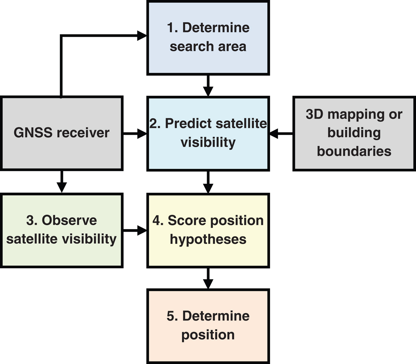
Figure 2. Shadow matching algorithm block diagram (adapted from Groves et al. (Reference Groves, Wang, Adjrad and Ellul2015)).
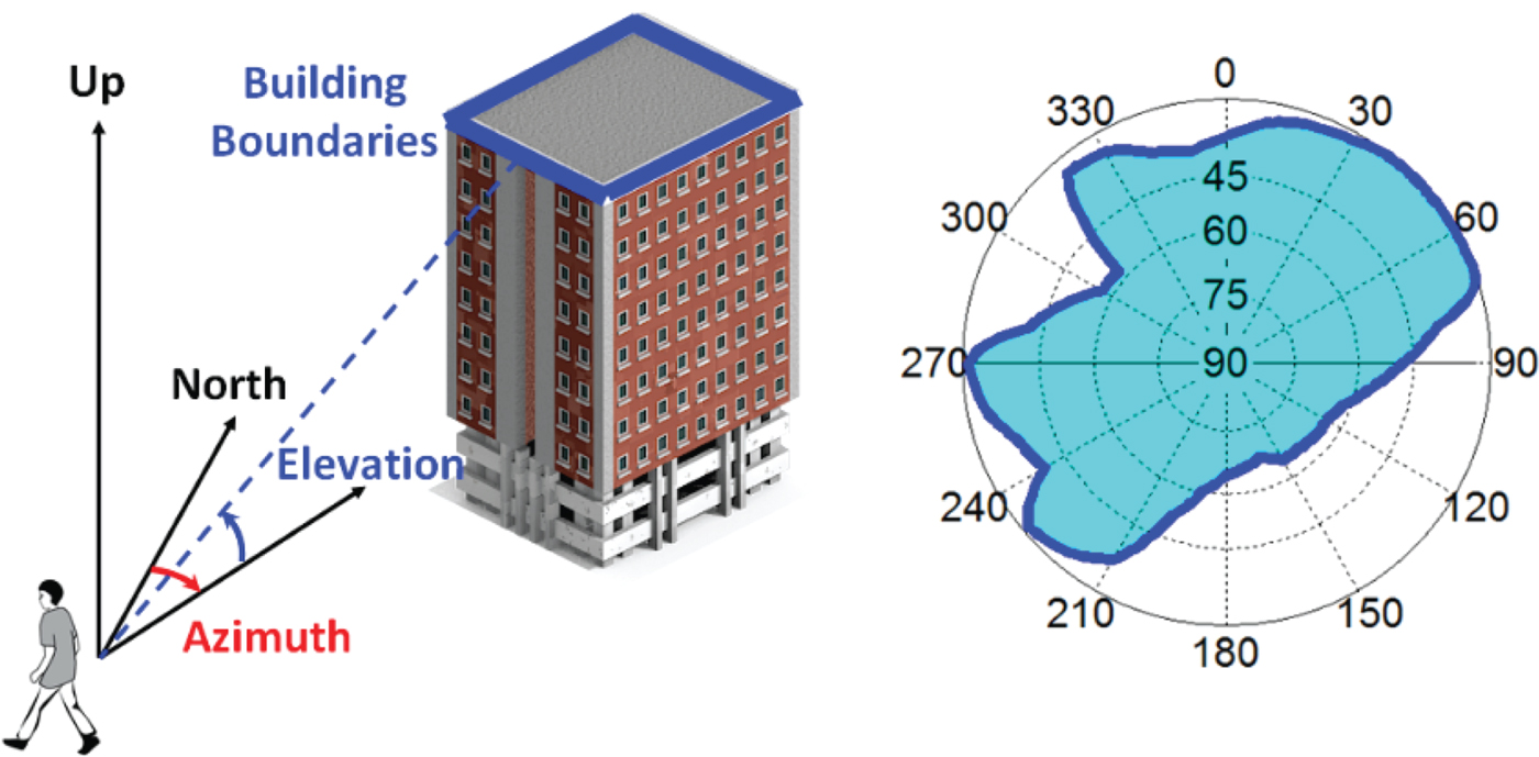
Figure 3. Building boundary definition (Wang et al., Reference Wang, Groves and Ziebart2013).
Figure 4 shows typical building boundaries in the form of elevation versus azimuth plots for a typical user at ten locations, randomly chosen on two adjacent straight-line streets (effectively taking as an example the case where the search area, centred at the 3DMA GNSS ranging-based solution, covers two different streets with different azimuths). For this example, we limit the number of grid points to ten for clarity of presentation. However, in the weighting algorithm, the process is performed for all outdoor grid points in the search area.

Figure 4. Building boundary representation - example of 10 grid points spread along two different streets: dashed lines representing the points belonging to one street and dotted lines for the grid points belonging to the second street, with a 57° difference in street azimuth (each colour represents a different grid point; five points are selected on each street).
As Figure 4 shows, the street azimuth angle, θ Street , can be extracted from the building boundaries. The street azimuth is the angle at which the elevation of the building boundary is at a minimum, i.e. there are no buildings directly in front. It is effectively the along-street direction with respect to North. For a straight street, there will be another minimum at approximately θ Street + 180° if the viewpoint is in the middle of the street. There are many possible viewpoints within the shadow matching search area, noting that indoor locations are excluded. Therefore, a viewpoint for inference of θ Street is selected at which the two azimuths at the two building boundary minima are 180 ± 1° apart. θ Street is set to whichever of the two minima has the lowest elevation (if the elevations are the same, the minima between 0 and 180° is selected).
In practice, there will usually be several streets in the search area and so each candidate position needs to be associated with a particular street. Figure 5 illustrates the case of search area grid points falling on two parallel streets. Firstly, a street azimuth angle is computed for each point and points with similar azimuths are grouped together. This will separate streets with different azimuths, but not parallel streets. Therefore, a second step is needed. For each group of points with similar azimuths, a set of viewpoints is extracted (shown as orange-filled circles on Figure 5). For each Easting coordinate, a maximum of two viewpoints are selected that meet the viewpoint criterion (i.e., the two building boundary minima are 180 ± 1° apart) - this effectively selects viewpoints that fall in the middle of the street. Where more than two candidates meet the viewpoint criterion, those within the search area with the highest and lowest Northing are selected, providing viewpoints on different streets (except where the parallel streets have an azimuth corresponding to north; in which case, the two viewpoints with largest easting coordinate difference are selected). Then, for each grid point in the group, the distance from each viewpoint in the across-street direction (i.e., θ Street + 90°) is computed. Each grid point is then associated to the viewpoint that is closest in the across-street direction, effectively allocating it to a particular street.
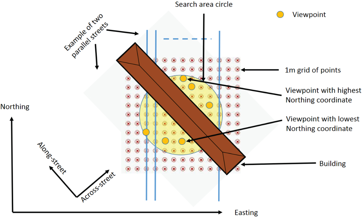
Figure 5. Association of candidate positions with streets (example of search area grid points falling on two parallel streets, shaded in grey).
Weighting factors for the GNSS ranging and shadow matching position solutions are determined in the along-street and across-street directions for each outdoor grid point, p, within the shadow matching search area based on the building-height-to-street-width ratio at that point. To find this ratio, the neighbouring points nearest to the buildings on the two sides of the street are first found by determining which points have the highest building boundary elevation along the two azimuths perpendicular to the street azimuth (stopping the search when an indoor point is encountered). The street width, w
p
, is the difference in across-street coordinates of these two points on either side of the street. The building height, $h_{B}^{p}$
, is then estimated using the building boundary angle,
$h_{B}^{p}$
, is then estimated using the building boundary angle, $\theta_{BB}^{p}$
, at the candidate position along the azimuth perpendicular to the street azimuth, together with the across-street distance, Δ w
p
, to the point nearest the building determined previously. The building height-to-street-width ratio is then estimated as
$\theta_{BB}^{p}$
, at the candidate position along the azimuth perpendicular to the street azimuth, together with the across-street distance, Δ w
p
, to the point nearest the building determined previously. The building height-to-street-width ratio is then estimated as $\delta_{hw}^{p} = h_{B}^{p} /w^{p} = (\Delta w^{p}/w^{p}) \tan (\theta_{BB}^{p})$
. In practice, both the street azimuths and the height-to-width ratios can be pre-computed and stored with the building boundaries.
$\delta_{hw}^{p} = h_{B}^{p} /w^{p} = (\Delta w^{p}/w^{p}) \tan (\theta_{BB}^{p})$
. In practice, both the street azimuths and the height-to-width ratios can be pre-computed and stored with the building boundaries.
The weighting matrices for point p are then
 $${\bf W}_{S,p}^{EN} = {\bf C}_{Ap}^{EN} \left( {\matrix{ {1 \over 1+{\delta_{hw}^p}^2} & 0 \cr 0 & {{\delta_{hw}^p}^2 \over 1+{\delta_{hw}^p}^2} }} \right) {\bf C}_{EN}^{Ap} \qquad {\bf W}_{R,p}^{EN} = {\bf C}_{Ap}^{EN} \left( {\matrix{ {{\delta_{hw}^p}^2 \over 1+{\delta_{hw}^p}^2} & 0 \cr 0 & {1 \over 1+{\delta_{hw}^p}^2} }} \right) {\bf C}_{EN}^{Ap},$$
where ${\bf C}_{Ap}^{EN}$
is the coordinate transformation matrix from the point p (along-street, across-street) frame to an (easting, northing) frame and is given by
${\bf C}_{Ap}^{EN}$
is the coordinate transformation matrix from the point p (along-street, across-street) frame to an (easting, northing) frame and is given by
 $${\bf C}_{Ap}^{EN} =\left( {\matrix{ {\sin \theta_{Street}^p } & {\cos \theta_{Street}^p } \cr {\cos \theta_{Street}^p } & {-\sin \theta_{Street}^p} }} \right),$$
where $\theta_{Street}^{p}$
is the azimuth angle of the street to which point p belongs. Note that
$\theta_{Street}^{p}$
is the azimuth angle of the street to which point p belongs. Note that ${\bf C}_{EN}^{Ap} = {{\bf C}_{Ap}^{EN}}^{\rm T}$
.
${\bf C}_{EN}^{Ap} = {{\bf C}_{Ap}^{EN}}^{\rm T}$
.
The overall weighting matrices for the shadow matching and GNSS ranging position solutions are then obtained by weighting the matrices for the individual points according to the shadow matching scores of each point. Thus,
 $${\bf W}_S^{EN} = {\sum\limits_{p=1}^{n_s} \Lambda_{Sp}^2 {\bf W}_{S,p}^{EN} \over \sum\limits_{p=1}^{n_s} \Lambda_{Sp}^2}, \qquad {\bf W}_R^{EN} = {\sum\limits_{p=1}^{n_s} \Lambda _{Sp}^2 {\bf W}_{R,p}^{EN} \over \sum\limits_{p=1}^{n_s } \Lambda_{Sp}^2},$$
where n s is the total number of grid points in the shadow matching search area and Λ Sp is the shadow matching score of point p, as defined in Section 2.2.
4. EXPERIMENTAL RESULTS
Measurements using a Sony Xperia smartphone and u-blox EVK M8T GNSS receiver were collected in January 2016. Two rounds of data collection were performed at 14 and 18 sites in central London, using the smartphone and u-blox receiver, respectively. All smartphone data collection was collocated with the corresponding u-blox data collection. The sites were paired with data collected on opposite sides of the street on the edge of the footpath next to the road. The truth was established to decimetre-level accuracy using a 3D city model to identify landmarks and a tape measure to measure the distance of the user position from those identified landmarks. The two rounds of data at each site were separated by approximately two hours, ensuring that the satellite positions in the two datasets were independent. The first dataset was used for calibrating the shadow matching algorithm for the smartphone and u-blox antenna and receiver characteristics using the procedure described in Wang et al. (Reference Wang, Groves and Ziebart2015), while the second dataset was used for testing the positioning algorithms. Four minutes of data (logging at 1 Hz) were collected at each site on each round. Figure 6 illustrates the measurement sites (smartphone data was not collected at sites 1N, 1S, 9N, 9S).

Figure 6. Data collection sites in the City of London (GoogleTM Earth).
A 3D city model of the area, from Ordnance Survey (OS), was used to generate the building boundary data used for the subsequent analysis (Adjrad and Groves, Reference Adjrad and Groves2017). The model is stored in the Virtual Reality Modelling Language (VRML) format. Figure 7 illustrates the 3D model used in this study.

Figure 7. The 3D model of City of London used in the experiments.
Figure 8 (Left) shows the u-blox receiver LOS and NLOS SNR distributions averaged across all of the experimental sites. Both direct LOS signals, shown in red, and NLOS signals, shown in blue, were received at every test site. In Figure 8 (Right), the blue crosses show the probability that a signal is direct LOS for each value of SNR derived from the experimental data. Figure 9 shows the corresponding information for the smartphone device.
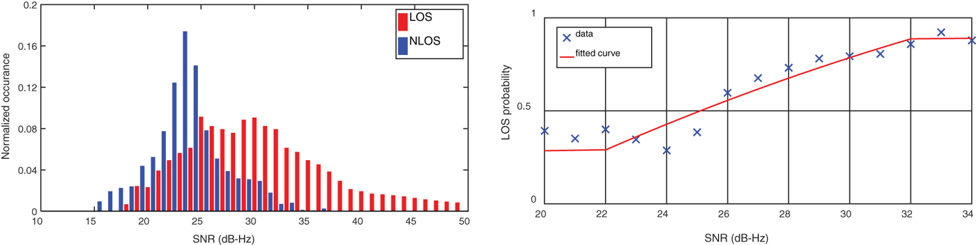
Figure 8. Normalised SNR distribution of LOS and NLOS signals across all sites (Left) and probability of LOS (Right) from the u-blox data.

Figure 9. Normalised SNR distribution of LOS and NLOS signals across all sites (Left) and probability of LOS (Right) from the smartphone.
For shadow matching satellite visibility scoring (see Section 2.2), the probability that a received signal is direct LOS is modelled as a function of the received SNR, s, using (Wang et al., Reference Wang, Groves and Ziebart2015)
 $$p\lpar LOS \vert SNR = s \rpar = \matrix{ {p_{o-\min}} \hfill & {s < s_{\min}} \hfill \cr {a_2 s^2 + a_1 s + a_0} &{s_{\min} < s < s_{\max}} \cr {p_{o - \max}} \hfill & {s_{\max} < s} \hfill} ,$$
where p o−min and p o−max are, respectively, the minimum and maximum probabilities of the observed signal being LOS; s min and s max are, respectively, the minimum and maximum SNRs at which the quadratic function applies and a 0, a 1, and a 2 are the coefficients of that function. New values of these coefficients for the u-blox EVK M8T receiver and Sony Xperia smartphone were derived by fitting this function to the experimental data, using the building boundaries at the true position to determine which measurements were direct LOS and which NLOS. Table 1 lists the values used for the shadow matching results presented here, while the red lines in Figure 8 (Right) and Figure 9 (Right) depict the functions for the two receivers. Note that p o−min and p o−max take the values of the quadratic function at s min and s max , respectively. Suitable values of s min and s max were determined by a combination of visual inspection of the data and examination of the residuals of the quadratic function fit to the data within these bounds.
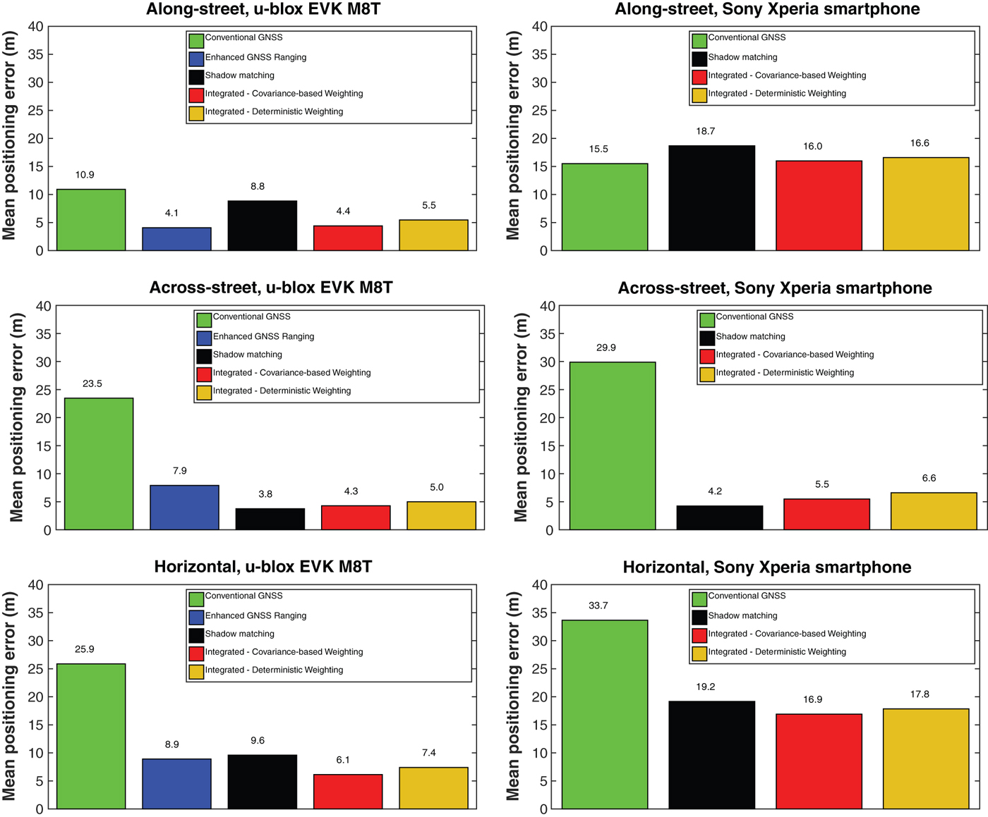
Figure 10. u-blox receiver and Smartphone along-street, across-street and overall horizontal RMS positioning error using individual and integrated approaches.
Table 1. Coefficients of LOS probability model.

The calibration data was also used to determine values for p(LOS| BB) by running the shadow matching algorithm with different values. Best performance was obtained with values between 0·75 and 0·85 for signals predicted to be direct LOS and between 0·15 and 0·25 for signals predicted to be NLOS.
Figure 10 shows the along-street, across-street and overall horizontal RMS positioning error using the testing data from both the u-blox GNSS receiver and the smartphone. Tables 2 and 3 summarise these error statistics. The scaling factors values used in Equation (20) to determine the covariance of the shadow matching position solution are S 0x = 2·3, S 0y = 2·3 for the u-blox receiver and S 0x = 2·2, S 0y = 2·6 for the smartphone.
Table 2. Summary of positioning results using u-blox EVK M8T receiver.
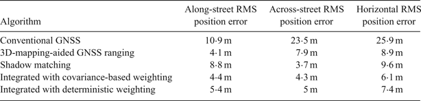
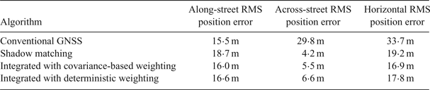
Table 3. Summary of positioning results using Sony Xperia smartphone.
Comparing the 3DMA integrated GNSS solution with the conventional GNSS solution, it can be seen that a substantial improvement in both along-street and across-street accuracy is achieved with the u-blox receiver. The smartphone GNSS receiver chip does not output pseudo-range measurements to the Application Programming Interface (API), so the 3DMA GNSS ranging algorithms cannot be implemented. Instead, shadow matching was integrated with the smartphone's conventional GNSS solution. As a result, the integrated solution is only better than the conventional solution in the across-street direction, not the along-street direction. Comparing the smartphone and u-blox results shows that a new smartphone GNSS interface that provides pseudo-ranges would enable a substantial improvement in position accuracy in dense urban areas.
5. CONCLUSIONS
Both 3D-mapping-aided GNSS ranging and shadow matching were integrated to realise an intelligent urban positioning system, whereby the across-street position is determined mainly by shadow matching and the along-street position mainly by ranging-based GNSS positioning. To ensure that shadow matching information is weighted correctly in the integrated position solution, a method to determine the covariance of the shadow matching solution was developed. The covariance of the 3DMA GNSS ranging solution was similarly determined. An alternative deterministic weighting algorithm, based on street azimuth derived from the 3D city model, was also developed.
The first performance assessment of shadow matching integrated with GNSS ranging has been conducted. GPS and GLONASS data were recorded at multiple locations within central London using a u-blox EVK-M8T GNSS receiver and a Sony Xperia smartphone. The results show that the Intelligent Urban Positioning integrated approach outperforms both GNSS ranging-based positioning and shadow matching, with the covariance-based weighting performing slightly better than the deterministic weighting. Using covariance-based weighting, the overall RMS horizontal accuracy obtained using the u-blox receiver was 6·1 m, compared to 25·9 m using conventional GNSS positioning, a factor of four improvement.
For the smartphone, it was only possible to integrate shadow matching with conventional GNSS positioning as pseudo-ranges were not output by this device so 3DMA GNSS ranging algorithms could not be implemented. The RMS horizontal accuracy was 16·9 m using the integrated approach, compared with 33·7 m using conventional GNSS positioning. The new smartphone GNSS receiver interface under development by Google will enable 3DMA GNSS ranging to be implemented with a consequent improvement in performance.
6. FUTURE WORK
The next stage of the current project is the development of a new 3DMA GNSS ranging algorithm that scores an array of candidate position solutions using separate LOS/NLOS predictions from the 3D city model at each individual point. Thus, the position error distribution is no longer approximated to a multivariate Gaussian distribution. The scores from the new 3DMA GNSS ranging algorithm can then be combined with the shadow matching scores for the same candidate positions and a joint position solution derived from the ensuing distribution. This hypothesis-domain integration approach does not need to make assumptions about the underlying position error distributions. Preliminary results were presented in Adjrad and Groves (Reference Adjrad and Groves2016) while this paper was under review.
Other challenges to address include (Groves et al., Reference Groves, Wang, Adjrad and Ellul2015):
-
• Extension from single-epoch to multi-epoch positioning, including determination of the optimum filtering strategy, e.g. a grid filter, a particle filter or a multi-hypothesis Kalman filter;
-
• Determination of the effects on performance of out-of-date mapping, such as missing buildings, and unpredictable features, such as large passing vehicles, and development of outlier detection techniques to mitigate them;
-
• Assessment of the impact on performance of 3D mapping quality, including different roof representations and levels of detail;
-
• A full assessment of the error characteristics of shadow matching and 3DMA ranging and appropriate adaptation of the candidate position scoring schemes and search area determination.
In the long term, advanced GNSS should be integrated with other navigation and positioning technologies for maximum reliability across a range of different challenging environments. This needs to be part of a paradigm shift. Instead of designing a single-technology navigation or positioning system, the philosophy should be to use as much information as can be cost-effectively obtained from many different sources to determine a navigation solution that is as accurate and reliable as possible. This requires many challenges to be addressed, including how to integrate many different navigation and positioning technologies when the necessary expertise is spread across multiple organisations (Groves, Reference Groves2014), and how to adapt a multi-sensor navigation system in real time to changes in the environmental and behavioural context (Groves et al., Reference Groves, Martin, Voutsis, Walter and Wang2013).
ACKNOWLEDGEMENTS
This work is funded by the Engineering and Physical Sciences Research Council (EPSRC) project EP/L018446/1, Intelligent Positioning in Cities using GNSS and Enhanced 3D Mapping. The project is also supported by Ordnance Survey, u-blox and the Royal National Institute for Blind People.}


 Open access