

In recent years, psychology has been at the forefront of a broad movement across scientific disciplines to improve the quality and rigor of research methods and practices (Begley & Ellis, Reference Begley and Ellis2012; Button et al., Reference Button, Ioannidis, Mokrysz, Nosek, Flint, Robinson and Munafò2013; Ledgerwood, Reference Ledgerwood2016; McNutt, Reference McNutt2014; Nosek, Spies, & Motyl, Reference Nosek, Spies and Motyl2012; Nyhan, Reference Nyhan2015; see Spellman, Reference Spellman2015, for a helpful synopsis). The field as a whole is changing: Conversations about improving research practices have become mainstream, journals and societies are adopting new standards, and resources for improving methods and practices have proliferated across journal articles, book chapters, and online resources such as blogs and social media (Simons, Reference Simons2018). As attention to methodological issues has surged, researchers have become increasingly interested in understanding and implementing methodological tools that can maximize the knowledge they get from the work that they do.
At the same time, for the average researcher, it can be daunting to approach this new wealth of resources for the first time. You know that you want to understand the contours of recent developments and to learn as much as possible from the research you do, but where do you even begin? We think that one of the most important methodological skills to develop is how to calibrate your confidence in a finding to the actual strength of that finding.
In this tutorial, we seek to provide a toolbox of strategies that can help you do just that. If a finding is strong, you want to have a relatively high level of confidence in it. In contrast, if a finding is weak, you want to be more skeptical or tentative in your conclusions. Having too much confidence in a finding can lead you to waste resources chasing and trying to build on an effect that turns out to have been a false positive, thereby missing opportunities to discover other true effects. Likewise, having too little confidence in a finding can lead you to miss opportunities to build on solid and potentially important effects. Thus, in order to maximize what we learn from the work that we do as scientists, we want to have a good sense of how much we learn from a given finding.
We divide this tutorial into two main parts. The first part will focus on how to estimate statistical power, which refers to the likelihood that a statistical test will correctly detect a true effect if it exists (i.e., the likelihood that if you are testing a real effect, your test statistic will be significant). The second part will focus on type I error, which refers to the likelihood that a statistical test will incorrectly detect a null effect (i.e., the likelihood that if you are testing a null effect, your test statistic will be significant). Arguably, one of the central problems giving rise to the field’s so-called “replicability crisis” is that researchers have not been especially skilled at assessing either the statistical power or the Type I error rate of a given study – leading them to be overly confident in the evidential value and replicability of significant results (see Anderson, Kelley, & Maxwell, Reference Anderson, Kelley and Maxwell2017; Lakens & Evers, Reference Lakens and Evers2014; Ledgerwood, Reference Ledgerwood2018; Nosek, Ebersole, DeHaven, & Mellor, Reference Nosek, Ebersole, DeHaven and Mellor2018a; Open Science Collaboration, 2015; Spellman, Gilbert, & Corker, Reference Spellman, Gilbert and Corker2017; Pashler & Wagenmakers, Reference Pashler and Wagenmakers2012). For example, Bakker, van Dijk, and Wicherts (Reference Bakker, van Dijk and Wicherts2012) estimated the average statistical power in psychological experiments to be only 35%, and even large studies may have lower statistical power than researchers intuitively expect when measures are not highly reliable (see Kanyongo, Brook, Kyei-Blankson, & Gocmen, Reference Kanyongo, Brook, Kyei-Blankson and Gocmen2007; Wang & Rhemtulla, Reference Wang and Rhemtullain press). Meanwhile, common research practices can inflate the type I error rate of a statistical test far above the nominal alpha (typically p < .05) selected by a researcher (John, Loewenstein, & Prelec, Reference John, Loewenstein and Prelec2012; Simmons, Nelson, & Simonsohn, Reference Simmons, Nelson and Simonsohn2011; Wang & Eastwick, Reference Wang and Eastwickin press).
Importantly, you need a good estimate of both quantities – statistical power and type I error – in order to successfully calibrate your confidence in a given finding. That is because both quantities influence the positive predictive value of a finding, or how likely it is that a significant result reflects a true effect in the population.Footnote 1
For example, imagine that in the course of a typical year, a researcher has ten ideas that happen to be correct and ten ideas that happen to be incorrect (that is, she tests ten effects that are in fact true effects in the population and ten that are not). Let us focus on what happens to the correct ideas first. As illustrated in Figure 1, the statistical power of the researcher’s studies determines how many of these true effects will be detected as significant. If the studies are powered at 40% (left side of Figure 1), four out of ten studies will correctly detect a significant effect, and six out of ten studies will fail to detect the effect that is in fact present in the population. If the studies are powered at 90% (right side of Figure 1), nine out of ten studies will correctly detect the significant effect, and only one will miss it and be placed in the file drawer.
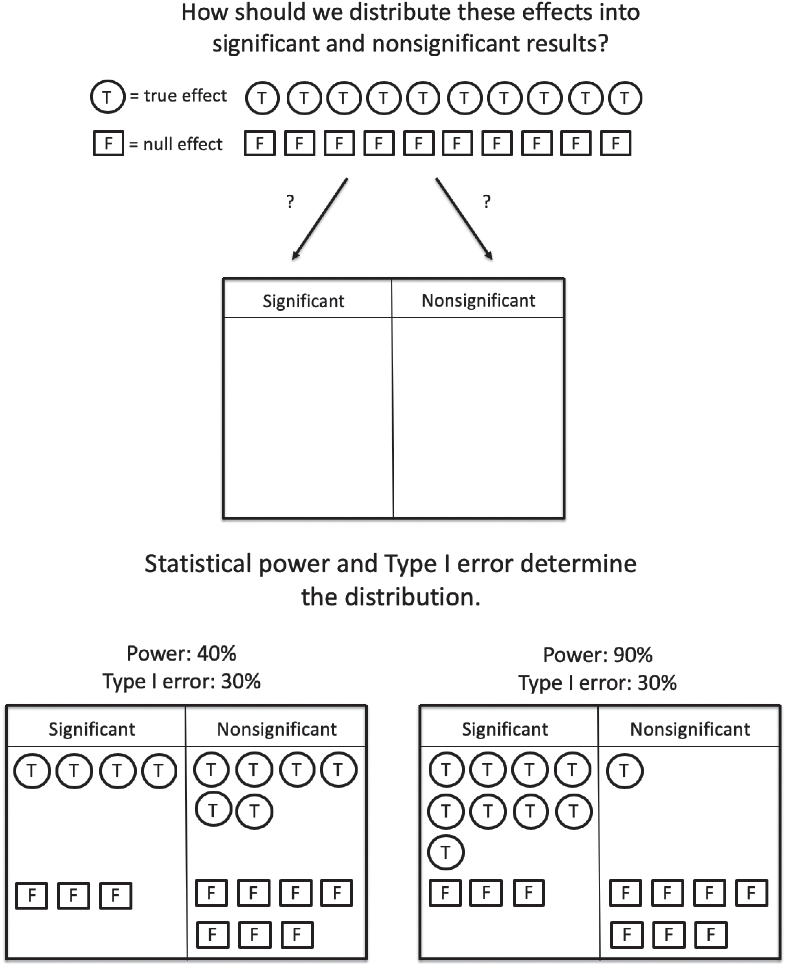
Figure 1. Consider the case of a researcher testing 10 true effects and 10 false effects. Perhaps they will follow up or publish significant results but leave nonsignificant results in a file drawer. The statistical power and type I error rate of the studies will determine how the effects are sorted into a set of significant results (follow up!) and a set of nonsignificant results (file drawer). Notice that because power is higher in the scenario on the right (vs. left), the likelihood that any one of the significant findings reflects a true effect in the population is also higher.
However, statistical power is only part of the story. Not all ideas are correct, and so let us focus now on the ten ideas that happen to be incorrect (that is, she tests ten effects that are in fact null effects in the population). As illustrated in Figure 1, the type I error rate of the researcher’s studies determines how many of these null effects will be erroneously detected. If the studies have a type I error rate of 30%, three of the ten null effects will be erroneously detected as significant, and the other seven will be correctly identified as nonsignificant.Footnote 2
The researcher, of course, does not know whether the effects are real or null in the population; she only sees the results of her statistical tests. Thus, what she really cares about is how likely she is to be right when she reaches into her pile of significant results and declares: “This is a real effect!” In other words, if she publishes or devotes resources to following up on one of her significant effects, how likely is it to be a correctly detected true effect, rather than a false positive? Notice that the answer to this question about the positive predictive value of a study depends on both statistical power and type I error rate. In Figure 1, the positive predictive value of a study is relatively low when power is low (on the left side): The likelihood that a significant result in this pool of significant results reflects a true effect is 4 out of 7 or 57%. In contrast, the positive predictive value of a study is higher when power is higher (on the right side of Figure 1): The likelihood that a significant result in this pool of significant results reflects a true effect is 9 out of 12, or 75%. Thus, if we are to understand how much to trust a significant result, we want to be able to gauge both the likely statistical power and the likely type I error rate of the study in question.
At this point, readers may wonder about the trade-off between statistical power and type I error, given that the two are related. For example, one way to increase power is to set a higher alpha threshold for significance testing (e.g., p < .10 instead < .05), but this practice will also increase type I error. However, there are other possible ways to increase power that do not affect the type I error rate (e.g., increasing sample size, improving the reliability of a measure) – and it is these strategies that we discuss below. More broadly, in this tutorial, we focus on providing tools to assess: (1) the likely statistical power; and (2) the likely type I error rate of a study result, and offer guidance for how to increase statistical power or constrain type I error for researchers who want to be able to have more confidence in a given result.
Part I: How to Assess Statistical Power
Develop Good Intuitions About Effect Sizes and Sample Sizes
One simple but useful tool for gauging the likely statistical power of a study is a well- developed sense of the approximate sample size required to detect various effects. Think of this as building your own internal power calculator that provides rough, approximate estimations.
You want to be able to glance at a study and think to yourself: “Hmm, that’s a very small sample size for studying this type of effect with this sort of design – I will be cautious about placing too much confidence in this significant result” or “This study is likely to be very highly powered – I will be relatively confident in this significant result.” In other words, it is useful to develop your intuitions for assessing whether you are more likely to be in a world that looks more like the left side of Figure 1 or in a world that looks more like the right side.
How do you build this internal calculator? You can start by memorizing some simple benchmarks. For a simple two-condition, between-subjects study, the sample size required to detect a medium effect size of d = .50 with 80% power is about N = 130 (65 participants per condition; see Figure 2. Notice that d = .50 is equivalent to r = .24 and h 2 = .06). To detect a large effect of d = .80 with 80% power requires about N = 50 (25 per condition). And to detect a small effect size of d = .20 with 80% requires about N = 800 (400 per condition; Faul, Erdfelder, Lang, & Buchner, Reference Faul, Erdfelder, Lang and Buchner2007).
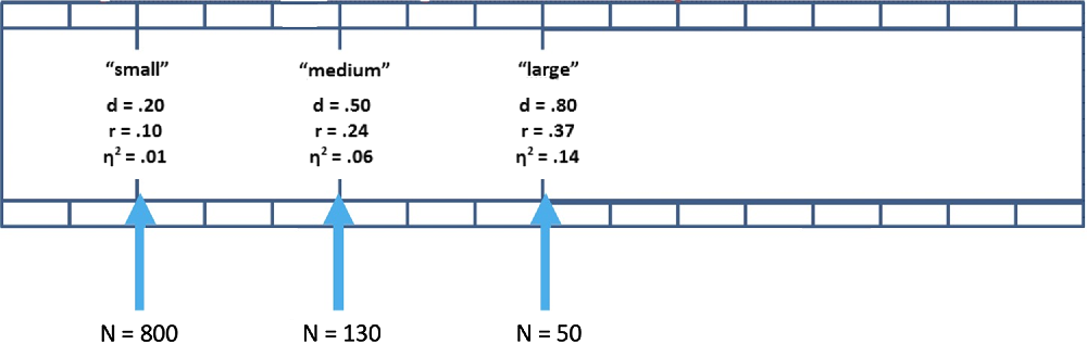
Figure 2. Sample sizes needed to achieve 80% power in a two-condition, between-subjects study. This figure helps you organize visually the effect size intuitions.
Next, start developing your sense of how big such effects really are. Cohen (Reference Cohen1992) set a medium effect size at d = .50 to “represent an effect likely to be visible to the naked eye of a careful observer” (p. 156), so a medium-sized effect is one that we might observe simply by watching people closely. A large effect size of d = .80 is typically an effect that even a casual observer would notice (e.g., the correlation between relationships satisfaction and breakup is approximately this magnitude; Le, Dove, Agnew, Korn, & Mutso, Reference Le, Dove, Agnew, Korn and Mutso2010). And a small effect size of d = .20 is typically too small to be seen with the naked eye (e.g., if you’re interested in testing a counterintuitive prediction that would be surprising to most people, it is likely to be a small effect if it is true). Pay attention to effect size estimates from meta-analyses and very large studies in your area of research to hone your intuitions within your particular research area.
Finally, keep in mind that interactions can require much larger sample sizes, depending on their shape. For example, imagine that you are interested in powering a two-group study to detect a medium-sized effect. You conduct Study 1 with a total sample size of N = 130 and find that indeed, your manipulation (let’s call it Factor A) significantly influences your dependent measure. Next, you want to know whether Factor B moderates this effect. How many participants do you need to have 80% power to detect an interaction in Study 2, where you manipulate both Factor A and Factor B in a 2 × 2 design?
As Table 1 illustrates, the answer depends on the shape of the interaction you expect (see Giner-Sorolla, Reference Giner-Sorolla2018; Ledgerwood, Reference Ledgerwood, Finkel and Baumeister2019). If you expect a knockout interaction (i.e., you think the effect you saw in Study 1 will appear in one condition of Factor B and disappear in the other), it turns out you need to quadruple the sample size you had in Study 1 to have 80% power to detect the interaction in Study 2. If you expect a perfect cross-over interaction (i.e., you think the effect you saw in Study 1 will appear in one condition of Factor B and reverse completely in the other), you need the same sample size you had in Study 1 to have 80% power to detect the interaction in Study 2 (although you will probably want to double the sample size to provide 80% power to detect each of the simple main effects). And if you expect a 50% attenuation (i.e., you think the effect you saw in Study 1 will appear in one condition of Factor B and be reduced to half its original size in the other), you need about 14 times the sample size you used in Study 1.
Table 1. Rules of thumb for powering a 2 × 2 between-subjects Study 2 that seeks to moderate a main effect observed in Study 1
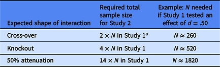
Note: In this illustration, Study 1 is powered to provide 80% power to detect a main effect. In Study 2, a researcher wants to test whether the effect observed in Study 1 is moderated by a second variable in a 2 × 2 between-subjects factorial design.
Strategies for a Planned Study
Conduct an a priori power analysis
The rules of thumb described above can be useful, but when you are planning your own study, you can conduct a formal, a priori power analysis to decide how many participants you need in order to achieve your desired level of power. In an a priori power analysis, you input your desired level of power (e.g., 80%), your planned statistical test (e.g., a t test comparing two between-subjects conditions), and your estimated effect size (e.g., d = .40), and the program tells you the necessary sample size (e.g., N = 200). The central challenge in this kind of power analysis is to identify a good estimate of the expected effect size.
Getting a good estimate of the expected effect size can be tricky for multiple reasons. First, effect size estimates (like any estimate) will fluctuate from one study to the next, especially when sample sizes are smaller (see Ledgerwood, Soderberg, & Sparks, Reference Ledgerwood, Soderberg, Sparks, Makel and Plucker2017, Figure 1, for an illustration). In other words, an effect size estimate from any given study can underestimate or overestimate the true size of an effect. Second, publication bias tends to inflate the effect sizes reported in a given literature. Historically, significant results were (and continue to be) more likely to be published, and null effects are more likely to be shuttled to a file drawer rather than shared with the scientific community (Anderson et al., Reference Anderson, Kelley and Maxwell2017; Ledgerwood, Reference Ledgerwood, Finkel and Baumeister2019; Rosenthal, Reference Rosenthal1979). Because any given study can underestimate or overestimate an effect size, and because overestimates are more likely to hit significance, publication bias effectively erases a sizable portion of underestimates from the literature. Therefore, a published effect size estimate is more likely to be an overestimate than an underestimate. And, when one averages the effect size estimates that do make it into the published literature, that average is usually too high (Anderson et al., Reference Anderson, Kelley and Maxwell2017).
To get around these issues, we have two options: a large study or a meta-analysis. In both cases, it is important to consider publication bias. The first option is to find an estimate of a similar effect from a large study (e.g., a total sample size of approximately N = 250 or larger for estimating a correlation between two variables or a mean difference between two groups; Schönbrodt & Perugini, Reference Schönbrodt and Perugini2013). If you find such a study, ask yourself whether the paper would have been published if it had different results (e.g., a paper that describes its goal as estimating the size of an effect may be less affected by publication bias than a paper that describes its goal as demonstrating the existence of an effect). The second option is to find an estimate of a similar effect from a meta-analysis. Meta-analyses aggregate results of multiple studies, so their estimates ought to be more accurate than an estimate from a single study. However, because they also sample studies from the literature, they can overestimate the size of an effect. For this reason, look for meta-analysis that carefully model publication bias (e.g., by using sensitivity analyses that employ various models of publication bias to produce a range of possible effect size estimates; McShane, Bockenholt, & Hansen, Reference McShane, Böckenholt and Hansen2016; see Ledgerwood, Reference Ledgerwood, Finkel and Baumeister2019, for a fuller discussion).
By identifying a good estimate of the expected effect size, such as those from large studies and meta-analyses that account for publication bias, we can conduct a priori power analyses that will be reasonably accurate. You can conduct an a priori power calculation using many simple-to-use programs, such as G*Power (Faul et al., Reference Faul, Erdfelder, Lang and Buchner2007); PANGEA (Westfall, Reference Westfall2016) for general analysis of variance (ANOVA) designs and pwrSEM (Wang & Rhemtulla, Reference Wang and Rhemtullain press) for structural equation models.
Of course, sometimes it is not possible to identify a good effect size estimate from a large study or meta-analysis that accounts for publication bias. If your only effect size estimate is likely to be inaccurate and/or biased (e.g., an effect size estimate from a smaller study), you can use a program that accounts for uncertainty and bias in effect size estimates (available online at https://designingexperiments.com/shiny-r-web-apps under the penultimate heading, “Bias and Uncertainty Corrected Sample Size for Power” or as an R package; see Anderson et al., Reference Anderson, Kelley and Maxwell2017).
Identify the biggest sample size worth collecting
In other situations, you are simply not sure what effect size to expect – perhaps you are starting a brand-new line of research, or perhaps the previous studies in the literature are simply too small to provide useful information about effect sizes. A useful option in such cases is to identify the smallest effect size of interest (often abbreviated to SESOI) and use that effect size in your power calculations (Lakens, Reference Lakens2014). In other words, if you only care about the effect if it is at least medium in size, you can power your study to detect an effect of d = .50.
Basic researchers often feel reluctant to identify a SESOI, because they often care about the direction of an effect regardless of its size (e.g., competing theories might predict that a given manipulation will increase or decrease levels on a given dependent measure, and a basic researcher might be interested in either result regardless of the effect size). However, with a minor tweak, the basic concept becomes useful to everyone. If identifying a SESOI feels difficult, identify instead the largest sample you would be willing to collect to study this effect.
Let’s call this the “Biggest Sample Size Worth Collecting”, or BSSWC. For example, if you decide that a given research question is worth the resources it would take to conduct a two-group experiment with a total of N = 100 participants, you are effectively deciding that you are only interested in the effect if it is at least d = .56 (the effect size that N = 100 would provide about 80% power to detect). Notice, then, that a BSSWC of 100 participants is equivalent to a SESOI of d = .56 – they are simply two different ways of thinking about the same basic idea. Notice, too, that it is worth making the connection between these two concepts explicit. For example, a social psychologist might consider whether the effect they are interested in studying is larger or smaller than the average effect studied in social-personality psychology (r = .21 or d = .43; see Richard, Bond, & Stokes-Zoota, Reference Richard, Bond and Stokes-Zoota2003). Unless they have a reason to suspect their effect is much larger than average, they may not want to study it with a sample size of only N = 100 (because they will be under-powered; see Figure 1).
Conserve resources when possible: Sequential analyses
Once you have determined the maximum sample size you are willing to collect (either through an a priori power analysis or by determining the maximum resources you are willing to spend on a given study), you can conserve resources by using a technique called sequential analysis. Sequential analyses allow you to select a priori the largest sample size you are willing to collect if necessary as well as middle points where you would stop data collection earlier if you could (Lakens & Evers, Reference Lakens and Evers2014; Proschan, Lan, & Wittes, Reference Proschan, Lan and Wittes2006). For example, if you have a wide range of plausible effect size estimates and are unsure about how many participants to run, but you know you are willing to collect a total sample size of N = 600 to detect this particular effect, a sequential analysis may be the best option. Sequential analyses are planned ahead of time, before looking at your results, and preserve a maximum type I error rate of 5%. In contrast, if you check your data multiple times without using a formal sequential analysis, type I error rates inflate (see Sagarin, Ambler, & Lee, Reference Sagarin, Ambler and Lee2014; Simmons et al., Reference Simmons, Nelson and Simonsohn2011).
To conduct a sequential analysis, you would first decide how many times you will want to check your data before reaching your final sample size – in our example, N = 600. Each additional check will reduce power by a small amount in exchange for the possibility of stopping early and conserving resources. Imagine that you decide to divide your planned sample into three equal parts, so that you conduct your analysis at n = 200, n = 400 and N = 600 participants (you can follow this example in Table 2). You would then pause data collection at each of these points and check the results. If the p value of the analysis is less than a predetermined alpha threshold (see Table 2), you would determine that the test is statistically significant. If it is greater than the threshold, you would continue collecting data up until the final sample size of N = 600.
Table 2. Alpha thresholds for sequential analyses
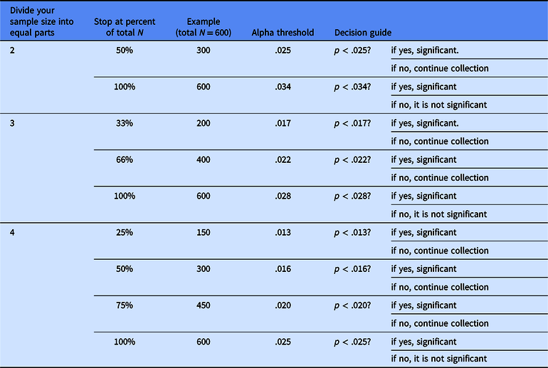
Note: Once you have planned your total sample size and how many times you will want to stop and check the results, use this table to determine the alpha cut-off thresholds you will use to determine significance at each planned analysis time point.
For instance, imagine that you collect the first planned set of 200 participants, or 33% of the total N. You pause data collection and analyze the data; if the p value of the focal analysis is below the first alpha threshold of .017, the result is significant and you can stop data collection early (saving 400 participants). If the p value of the focal analysis is not below .017, you continue to collect data from 200 more participants. When you check the results again, if the p value is below the second alphas threshold of .022, the result is significant and you can stop data collection early (saving 200 participants). If the p value is not below .022, you continue to collect data from 200 more participants and then conduct the focal analysis one final time on the total sample of 600 participants. If the p value is below .028, the result is significant. If it is not below .028, the result is not significant. In either case, you stop collecting data because you have reached your final planned sample size.
Importantly, by computing specific, adjusted alpha thresholds depending on the planned number of stopping points, sequential analysis enables researchers to check the data multiple times during data collection while holding the final type I error rate at a maximum of .05. This allows you to balance the goals of maximizing power and conserving resources. Table 2 provides the alpha thresholds for common sequential analyses where a researcher wants to divide their total planned sample (of any size) into 2–4 equal parts and hold their type I error rate at .05 or below (for an example of how to write up a sequential analysis, see Sparks & Ledgerwood, Reference Sparks and Ledgerwood2017). If you want to stop more frequently or at unevenly spaced points, you can use the GroupSeq R package and step-by-step guide provided by Lakens (Reference Lakens2014; resources available at https://osf.io/qtufw/) to compute other alpha thresholds.
Consider multiple approaches to boosting power
After conducting an a priori power analysis, you may find that to have your desired level of power, you need a larger sample size than you initially imagined. However, it is not always possible or practical to collect large sample sizes. You may be limited by the number of participants available to you (especially when studying hard-to-reach populations) or by the finite money and personnel hours that you have to spend on collecting data. Whatever the situation, all researchers face trade-offs and constraints based on resources.
Given such constraints, it is often useful to consider multiple approaches to boosting the power of a planned study. When possible and appropriate, making a manipulation within-subjects instead of between-subjects can dramatically boost the power of an experiment (see Greenwald, Reference Greenwald1976; Rivers & Sherman, Reference Rivers and Sherman2018). Likewise, you can increase power by strengthening a manipulation and by improving the reliability of your measures (see e.g., Ledgerwood & Shrout, Reference Ledgerwood and Shrout2011). In addition, it is sometimes possible to select ahead of time a planned covariate that correlates strongly with the dependent measure of interest (e.g., measuring extraversion as a covariate for a study that examines self-esteem as the focal dependent variable; see Wang, Sparks, Gonzales, Hess, & Ledgerwood, Reference Wang, Sparks, Gonzales, Hess and Ledgerwood2017). Finally, one of the most exciting developments in the “cooperative revolution” created by the open science movement is the proliferation of opportunities for large-scale collaborations (e.g., the Psychological Science Accelerator, ManyLabs, ManyBabies, and StudySwap; see Chartier, Kline, McCarthy, Nuijten, Dunleavy, & Ledgerwood, Reference Chartier, Kline, McCarthy, Nuijten, Dunleavy and Ledgerwood2018). When it simply is not feasible to study the research question you want to study with high statistical power, consider collaborating across multiple labs and aggregating the results.
Strategies for an Existing Study
Conduct a sensitivity analysis
When you want to assess the statistical power of an existing study (e.g., a study published in the literature or a dataset you have already collected), you can conduct a type of power analysis called a sensitivity analysis (Cohen, Reference Cohen1988; Erdfelder, Faul & Buchner, Reference Erdfelder, Faul, Buchner, Everitt and Howell2005). In a sensitivity analysis, you input the actual sample size used in the study of interest (e.g., N = 60), the statistical test (e.g., a t test comparing two between-subjects conditions), and a given level of power (e.g., 80%), and the program tells you the effect size the study could detect with this level of power (e.g., d = .74). The central goal for this kind of power analysis is to provide a good sense of the range of effect sizes that an existing study was adequately powered to detect.
For example, perhaps you have already conducted a study in which you simply collected as many participants as resources permitted, and you ended up with a total sample of N = 164 participants in a two-group experimental design. You could conduct sensitivity analyses to determine that your study had 60% power to detect an effect size of d = .35 and 90% power to detect an effect of d = .51. Armed with the effect size intuitions we discussed in an earlier section, you could then ask yourself whether the effect size you are studying is likely to be on the smaller side or on the larger side (e.g., is it an effect that a careful observer could detect with the naked eye?). By thinking carefully about this information, you can gauge the likely statistical power of your study (e.g., is it more like the left side or the right side of Figure 1?) and calibrate your confidence in the statistical result accordingly.
Don’t calculate “post-hoc” or “observed” power
Many types of power analysis software also provide an option for computing power called post hoc power or observed power. This type of power analysis is highly misleading and should be avoided (Gelman & Carlin, Reference Gelman and Carlin2014; Hoenig & Heisey, Reference Hoenig and Heisey2001). In a post hoc power analysis, you input the effect size estimate from a study as if it is the true effect size in the population. However, as discussed earlier, a single study provides only one estimate of the true population effect size, and this estimate tends to be highly noisy: It can easily be far too high or far too low (see Figure 1 in Ledgerwood et al., Reference Ledgerwood, Soderberg, Sparks, Makel and Plucker2017; Schönbrodt & Perugini, Reference Schönbrodt and Perugini2013). Furthermore, because researchers tend to be more interested in following up on and publishing significant results, and because a study is more likely to hit significance when it overestimates (vs. underestimates) an effect size, researchers are especially likely to conduct post hoc power analyses with overestimated effect size estimates.
The result of using post-hoc power is an illusion of a precise power estimate that in fact is (1) highly imprecise and (2) redundant with the p value of the study in question. In other words, post-hoc power or observed power appears to provide a new piece of very precise information about a study, when in fact it provides an already known piece of imprecise information. It is loosely akin to attempting to gauge the likelihood that a coin flip will result in “heads” rather than “tails” based on flipping the coin, observing that the result is “heads,” and then deciding based on this observation that the coin flip must have been very likely to result in the outcome you saw. Thus, post-hoc power or observed power ultimately worsens your ability to calibrate your confidence to the strength of a result.
Part II: How to Assess Type I Error Rates
As Figure 1 illustrates, if we want to correctly calibrate our confidence in a significant result, we want to be able to gauge not only the likely statistical power of the test in question, but also its likely type I error rate. Researchers often assume that their type I error rate is simply set by the alpha cut-off against which a p value is compared (traditionally, p < .05). In reality, however, the likelihood of mistakenly detecting a significant effect when none exists in the population can be inflated beyond the nominal alpha rate (.05) by a number of factors.
Understand How Data-Dependent Decisions Inflate the Type I Error Rate
Perhaps most importantly, the type I error rate can inflate – often by an unknown amount – when the various decisions that a researcher makes about how to construct their dataset and analyze their results are informed in some way by the data themselves. Such decisions are called data-dependent (or often “exploratory,” although this term can have multiple meanings and so we avoid it here for the sake of clarity). For example, if a researcher decides whether or not to continue collecting data based on whether their primary analysis hits significance, the type I error rate of that test will inflate a little (if they engage in multiple rounds of such “optional stopping,” type I error can increase substantially; see Sagarin et al., Reference Sagarin, Ambler and Lee2014). Likewise, running an analysis with or without a variety of possible covariates until one hits significance can inflate type I error (see Wang et al., Reference Wang, Sparks, Gonzales, Hess and Ledgerwood2017), as can testing an effect with three slightly different dependent measures and reporting only the ones that hit significance. In fact, even the common practice of conducting a 2 × 2 factorial ANOVA and reporting all effects (two main effects and an interaction) has an associated type I error rate of about 14% rather than the 5% researchers typically assume (see Cramer et al., Reference Cramer, van Ravenzwaaij, Matzke, Steingroever, Wetzels, Grasman and Wagenmakers2016). In all of these cases, the problem arises because there are multiple possible tests that a researcher could or does run to test their research question (e.g., a test on a subsample of 100 and a test on a subsample of 200; a test on one dependent measure versus a test on a different dependent measure). When the decision about which test to run and report is informed by knowledge of the dataset in question, the type I error rate starts to inflate (see Gelman & Loken, Reference Gelman and Loken2014; Simmons, Nelson, & Simonsohn, Reference Simmons, Nelson and Simonsohn2011).
Clearly Distinguish Between Data-Dependent and Data-Independent Analyses with a Preanalysis Plan
Of course, the fact that data-dependent analyses inflate type I error does not mean that you should never let knowledge of your data guide your decisions about how to analyze your data. Data-dependent analyses are important to get to know your data and to help generate new hypotheses and theories. Moreover, in some research areas, it is difficult or impossible to analyze a dataset without already knowing something about the data (e.g., political science studies of election outcomes; Gelman & Loken, Reference Gelman and Loken2014). Data-dependent analyses are often extremely useful, but we want to know that an analysis is data-dependent so that we can calibrate our confidence in the result accordingly.
Thus, an important tool to have in your toolkit is the ability to distinguish clearly between data-dependent and data-independent analyses. A well-crafted preanalysis plan allows you to do just that. A preanalysis plan involves selecting and writing down ahead of time the various researcher decisions that will need to be made about how to construct and analyze a dataset, before looking at the data. Writing down the decisions ahead of time is important to circumvent human biases in thinking and memory (Chaiken & Ledgerwood, Reference Chaiken and Ledgerwood2011; Nosek et al., Reference Nosek, Spies and Motyl2012) – after looking at the data, it is very easy to convince ourselves we actually intended to do these particular tests and make these particular decisions all along. By creating a record of which decisions were in fact data-independent, preanalysis plans allow researchers to distinguish between data-dependent and data-independent analyses. For example, if you write down ahead of time that you will include a carefully chosen covariate in your analysis and you follow that plan, you can rest assured that you have not unintentionally inflated your type I error rate (Wang et al., Reference Wang, Sparks, Gonzales, Hess and Ledgerwood2017). On the other hand, if you decide after looking at the data to include a different covariate or none at all, you can calibrate your confidence in that data-dependent analysis accordingly (e.g., being more tentative about that result until someone can test if it replicates).
Preanalysis plans thus enable you to plan your analyses with a constrained type I error rate, allowing you to know what this rate is. However, the plan is not a guarantee for keeping an alpha level below the desired rate (usually .05). If you plan multiple comparisons (e.g., you plan to test all effects in a two-way ANOVA; Cramer et al., Reference Cramer, van Ravenzwaaij, Matzke, Steingroever, Wetzels, Grasman and Wagenmakers2016) or inappropriate statistical tests (e.g., you use multiple regression rather than latent variables to test the incremental validity of a psychological variable, which can produce spurious results due to measurement error; see Westfall & Yarkoni, Reference Westfall and Yarkoni2016; Wang & Eastwick, Reference Wang and Eastwickin press), your type I error rate may be higher than you imagine. Also, it is important not to follow the plan blindly, and always check whether the assumptions of a statistical test are met given the data.
When constructing a preanalysis plan for the first time, it is often useful to start with a template designed for your type of research. For example, psychological researchers conducting experiments often find the AsPredicted.org template useful because it clearly identifies the most common researcher decisions that an experimental psychologist will need to make and provides clear examples of how much detail to include about each one. Other templates are available on OSF (see https://osf.io/zab38/), or you can create your own tailored to your own particular research context (see Table 3 for an example). Do not be surprised to find that you forget to record some researcher decisions the first time you create a preanalysis plan for a given line of research. It can be hard to anticipate all the decisions ahead of time. But even when a preanalysis plan is incomplete, it can help you clearly identify those analyses that were planned ahead of time and those that were informed in some way by the data.
Table 3. Common decisions to specify in a preanalysis plan
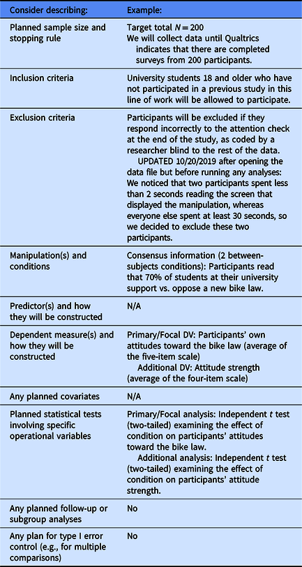
Note: Notice that although some templates ask you to identify a research question or prediction as a simple way to help readers understand the focus of your study, you can create a preanalysis plan even when you have no prediction about how your results will turn out (see Ledgerwood, Reference Ledgerwood2018). Notice too that preanalysis plans must be specific to be useful (e.g., if the dependent measure does not specify how many items will be averaged, it is not clear whether the decision about which items to include was made before or after seeing the data).
Distinguish Between Different Varieties of Preregistration and their Respective Functions
As described above, preanalysis plans can be very useful for clearly distinguishing between data-independent and data-dependent analyses. Preregistering a preanalysis plan simply means recording it in a public repository (e.g., OSF, AsPredicted.org, or socialscienceregistry.org). However, it is important to recognize that the term preregistration is used in different ways by different researchers both within and beyond psychology, and that these different definitions often map onto different goals or functions (Ledgerwood & Sakaluk, Reference Ledgerwood and Sakaluk2018; see also Navarro, Reference Navarro2019). Table 4 outlines the most common varieties of preregistration and their intended functions.
Table 4. Different definitions of preregistration and their intended purpose
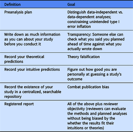
Researchers in psychology often use the term “preregistration” to mean a preanalysis plan, and advocate using this type of preregistration to reduce unintended type I error inflation and help researchers correctly calibrate their level of confidence or uncertainty about a given set of results (e.g., Nosek, Ebersole, DeHaven, & Mellor, Reference Nosek, Ebersole, DeHaven and Mellor2018a; Simmons, Nelson, & Simonsohn, Reference Simmons, Nelson and Simonsohn2017). But researchers in psychology and other disciplines also use the term “preregistration” to mean other practices that do not influence type I error (although they serve other important functions). Distinguishing between different varieties or elements of preregistration and thinking carefully about their intended purpose (and whether a given preregistration successfully achieves that purpose) is crucial if we want to correctly calibrate our confidence in a given set of results.
For example, researchers across disciplines sometimes use the term “preregistration” to mean a peer-reviewed registered report, where a study’s methods and planned analyses are peer reviewed before the study is conducted; in such cases, the decision about whether to publish the study is made independently from the study’s results (e.g., Chambers & Munafo, Reference Chambers and Munafo2013). This type of preregistration can help constrain type I error inflation (insofar as the analyses are specified ahead of time and account for multiple comparisons), while also achieving other goals like combatting publication bias (because the decision about whether to publish the study does not depend on the direction of the results). However, the reverse is not true: A preanalysis plan by itself does not typically combat publication bias (primarily because in psychology such plans are not posted in a public, centralized, easily searchable repository).
Similarly, researchers often talk about preregistration as involving recording a directional prediction before conducting a study (e.g., Nosek et al., Reference Nosek, Ebersole, DeHaven and Mellor2018a), which can be useful for theory falsification. However, writing down one’s predictions ahead of time does not influence type I error: The probability of a given result occurring by chance does not change depending on whether a researcher correctly predicted it ahead of time (Ledgerwood, Reference Ledgerwood2018). Thus, a researcher who records their predictions ahead of time without also specifying a careful preanalysis plan runs the risk of unintended type I error inflation (Nosek, Ebersole, DeHaven, & Mellor, Reference Nosek, Ebersole, DeHaven and Mellor2018b).
Thus, in order to correctly calibrate our confidence in a given study’s results, we need to know more than whether or not a study was “preregistered” – we need to ask how a study was preregistered. Did the preregistration contain a careful and complete preanalysis plan that fully constrained flexibility in dataset construction and analysis decisions? Did the plan successfully account for multiple comparisons? And did the researcher exactly follow the plan for all analyses described as data-independent? Thinking carefully and critically about preregistration will help you identify which of the goals (if any) listed in Table 4 have been achieved by a given study, and whether you should be more or less confident in that study’s conclusions.
Conclusion
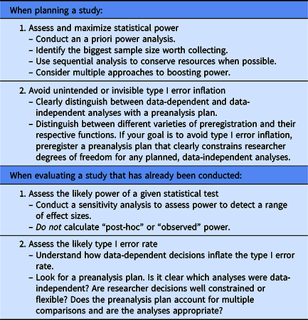
In this tutorial, we have discussed a number of strategies that you can use to calibrate the confidence you have in the results of your own studies as well as studies from other researchers (see Table 5). These strategies address typical issues researchers face when they try to assess the likely statistical power and type I error rate of a given study. By improving our ability to gauge statistical power and type I error, we can distinguish between study results that provide relatively strong building blocks for our research programs (those with high positive predictive value, as illustrated on the right side of Figure 1) and study results that provide more tentative evidence that needs to be replicated before we build on it (those with low positive predictive value, as illustrated on the left side of Figure 1). To help us get a better sense of the power of a study, we can develop good effect size intuitions; conduct a priori power analyses when we are in the planning phase of a project; and conduct sensitivity analyses when data has already been collected. To help us get a better sense of the type I error rate of a study, we can clearly distinguish between data-dependent (exploratory) and data-independent (confirmatory) analyses using a preanalysis plan; think critically about different varieties of preregistration; and evaluate whether a given preregistration successfully achieves its desired function(s). Together, these strategies can help improve our research methods as scientists, allowing us to maximize what we learn from the work that we do.
Table 5. Summary of recommendations
Financial support
None.


 Open access