


1. Introduction
Many countries are undertaking pension reforms to ensure the sustainability of their pension systems in an ageing society. Understanding how individuals respond to financial incentives is crucial for the design of retirement and pension policy and many recent studies have estimated how individuals respond to changes in the incentives.
Only few studies investigate the labour supply responses of couples to financial incentives for the couple. A seminal example is Baker (Reference Baker2002). For the Netherlands, Mastrogiacomo et al. (Reference Mastrogiacomo, Alessie and Lindeboom2004) investigated how the Dutch partner allowance (PA) affected couples' participation decisions. We use a more recent policy change to investigate the effect of the same PA on the retirement decisions of couples, exploiting its elimination in 2015. PA was a supplementary allowance (up to the full state pension (SP) for an individual in a couple, 50% of the minimum wage)Footnote 2 to the SP, paid to the partner who already reached the State Pension Age (SPA) if the other partner was younger than SPA and had low personal income from work or benefits. This allowance was introduced in 1985 to avoid poverty in couples with a (male) breadwinner above SPA and a spouse below SPA not doing paid work. In 2015, PA was abolished for new casesFootnote 3: those reaching SPA after 1 April 2015 (born after 1949) are not eligible.
The elimination of PA was motivated by the individualization of the pension system and the need to reduce the costs of public pensions. Improvement of the sustainability of the pension system is expected for two reasons: a reduction in pension expenditures and an increase in social contributions of younger partners who have more incentives to do paid work. The effectiveness of the reform depends on how couples respond to the change in financial incentives. Since PA is conditional on a low income of the younger spouse, it reduces the net reward for working for the younger partner, inducing a negative effect on the younger partner's labour supply during the time period that only the older partner has reached SPA (substitution effect). In addition, PA shifted the household life-cycle budget constraint, negatively affecting both spouses' labour supply (income effects), possibly even before the older partner reaches SPA. Moreover, complementarities in leisure and intra-household division of labour may lead to indirect effects on both partners' labour supply.
We analyse the effect of PA eligibility on the younger and older partners' retirement decisions by comparing couples in which the older partner reached their SPA immediately before (February–March 2015; cohort born just before 1950) or after (April–May 2015; cohort born just after 1949) the elimination. Cohorts born after 1949 were also affected by a reform in the early retirement (ER) scheme (the ER reform, ‘Wet VPL’) that essentially implied abolishing generous (actuarially very unfair) ER occupational pensions. In order to measure the effectiveness of the PA reform on older partners, we need to account for the effects of this ER reform, since the policy change applies to exactly the same birth cohorts of older partners. To account for the ER reform in the analysis of older partners, we apply a differences-in-differences approach and compare couples with one-person households, to whom PA never applies (briefly referred to as singles, from now on) born immediately before and shortly after 1 January 1950. Moreover, to account for indirect effects through a labour supply response of the partner, we refine this analysis distinguishing cases where the partner does or does not have an attachment to the labour market some years before approaching SPA – only for the former group, we can expect such indirect effects. Younger partners, on the other hand, all fall under the regime after the ER reform and we analyse their response comparing the groups who just fall and just do not fall under the new regime.
We use a rich administrative dataset that covers all Dutch residents and contains information on employment status as well as a large set of individual and household characteristics. Our findings clearly show that PA induced ER. According to our benchmark model, for older partners, PA eligibility increased the probability of retiring before age 63 by approximately 2.3 percentage points for men and by approximately 2.7 percentage points for women. For male younger partners, we find a small and insignificant negative effect of the PA, while for females, the PA option increased the probability to retired shortly before the older partner reaches SPA by approximately 11 percentage points. The effect is larger for those who initially (i.e., 5 years earlier) were part-time workers than for full-time workers.
The remainder of this paper is organized as follows. Section 2 reviews the literature. Section 3 explains the main characteristics of the Dutch pension system. Section 4 describes the data. In Section 5, we present our identification strategy and the econometric models. Section 6 discusses the main results. In Section 7, we analyse the validity of the identifying assumptions and carry out a sensitivity analysis. Conclusions are drawn in Section 8.
2. Literature review and theoretical background
Numerous studies have shown the importance of Social Security incentives for the timing of retirement. We focus on reduced form studies,Footnote 4 which often use policy changes to identify the causal effect of the financial incentives on retirement. Most of these studies have focused on incentives at the individual level (Gruber and Wise, Reference Gruber and Wise2004; Mastrobuoni, Reference Mastrobuoni2009), but some also examine the cross-effects on spouses (Coile, Reference Coile2004; Cribb et al., Reference Cribb, Emmerson and Tetlow2013; Lalive and Parrotta, Reference Lalive and Parrotta2017; Selin, Reference Selin2017; Stancanelli, Reference Stancanelli2017; Atalay et al., Reference Atalay, Barrett and Siminski2018).
Baker (Reference Baker2002) examines how couples´ labour supply responded to the introduction of the Spouse's Allowance (SA) in Canada in 1975, an allowance addressed to the younger partner but means-tested based on family income. Individuals in eligible couples responded to the incentives implied by the allowance by reducing participation. This effect was stronger for men than for women.
We investigate the effect of the PA in the Dutch pension system on the retirement decisions of couples, exploiting the PA's recent elimination. The design of the Dutch PA and the period of analysis differ substantially from those in Baker (Reference Baker2002). In Canada, the younger spouse could be entitled to SA from 60 to 64 years old. In the Netherlands, the only age limit is the SPA when younger spouses become entitled to their own public pension. While the Canadian SA is means-tested on family income, the Dutch PA was means-tested on the younger partner's income only.
Mastrogiacomo et al. (Reference Mastrogiacomo, Alessie and Lindeboom2004) investigated how the Dutch PA affected household participation decisions in the Netherlands using a structural model. Using policy simulations, they found that, compared to PA, a benefit independent of the younger partner's income would induce many younger partners to continue working after the older partner's SPA. We investigate the response of younger as well as older partners in a reduced form analysis exploiting the elimination of the PA.
Empirical evidence on the magnitude of the causal effect is very limited but useful to forecast the fiscal impact of future reforms. We, therefore, quantify the total effect of the PA on spouses' labour supply. Moreover, retirement decisions are influenced by non-rational and behavioural factors such as social norms, age anchors, peer effects and reference dependence. For instance, Behagel and Blau (Reference Behagel and Blau2012) and Vermeer (Reference Vermeer2016) find that it matters how the standard retirement age is framed. Moreover, complementarities in leisure and intra-household division of labour may play a role in the couple's joint retirement decisions (see, e.g., An et al., Reference An, Christensen and Datta Gupta2004). In the current paper, we do not aim at disentangling all these effects, but only estimate the total effect of (abolishing) PA on retirement decisions of both partners from 60 months before until 12 months (for younger partners) or 6 months (for older partners) after the older partner's SPA.
3. The Dutch pension system
As in many European countries, the Dutch pension system consists of three pillars: a state pension, (mandatory) occupational pensions, and individual private pensions.
3.1 First pillar: State Pension (SP)
The first pillar is the state pension (AOW, Algemene Ouderdoms Wet Footnote 5) that aims to provide a basic income (linked to the minimum wage) for everyone who has reached the statutory pension age (SPA).Footnote 6 Its financing scheme is a pay-as-you-go system. Everyone who has been a resident in the Netherlands from aged 15 to 65 years is eligible for SP after reaching the SPA (each year 2% of the full public pension benefit is accumulated). The rules for eligibility and for the amount of SP are very easy and published widely. Thus, every Dutch resident who makes a small effort to collect the information can fully anticipate receiving a given amount from a specific age.
The amount is determined by the official minimum wage level and depends on partnership status but not on earnings or employment history. It provides Dutch residents with a pension benefit that in principle guarantees 70% of the minimum wage for a person living alone and 50% for each partner in a couple (married or living together), so that a couple's SP income equals the minimum wage, corresponding to the minimum standard of living for a household with two adults.
3.1.1 Partner allowance
The Partner Allowance was linked to the SP until its elimination in 2015. It was based upon the traditional notion of a one-earner household, in which the older spouse was the only earner. Without PA or other additional income, such a household would end up in poverty when only the spouse would only receive the 50% of the minimum wage SP for an individual in a couple. Table A2 in the Appendix shows the state pension amounts including PA by partnership status. Partner allowance (PA, or supplementary SP) was paid to individuals who reached SPA while their partnerFootnote 7 was younger than SPA and had low own income from work and benefits. Without PA, the older spouse in this type of couple would receive 50% of the minimum wage and the younger spouse would not receive anything so that the couple's SP income would be below the minimum standard of living. The amount of the PA was 50% of the minimum wage, independent of previous earnings. With PA in place, the couple with non-working PA eligible spouse would therefore get 100% of the minimum wage in total – corresponding to the minimum living standard for a couple. Since August 2011, the amount of the PA could be reduced by up to 10% if the joint monthly income of both spouses (including State Pension and Partner Allowance) was €2,714 gross or more.
Figure 1 shows the PA amount by the younger partner's gross monthly income. The first €236.70 of partner's gross monthly earnings were disregarded; Two-thirds of earnings above €236.70 were deducted from the allowance; if the younger spouse's gross earnings exceeded €1,411.13 per month, no PA was paid. If the younger partner receives a pension, it was fully deducted from the allowance. If this was more than €782.95 gross per month, no PA was paid.

Figure 1. PA amount (€ per month) by the income of the younger partner (€ per month). Source: Own elaboration.
In 2015, PA was abolished for new cases: It is not paid if the older partner starts receiving SP on or after 1 April 2015 (i.e., the older partner is born after 31 December 1949). It is also not paid if the couple was formed after 1 January 2015 or was (due to the younger partner's income), not entitled to PA before 1 April 2015.
The elimination of the PA was first announced in 1995. Since it was announced well in advance, couples could anticipate it. For example, older husbands with wives not attached to the labour market could increase their labour supply already at an early stage because the reform reduces their income in the time between their own and their spouse's SPA, and thus reduces lifetime income (an income effect). Younger partners might change their work intentions after the older partner's SPA because the reform increases the reward for working in those years. This might induce them not to withdraw from the labour market at an earlier stage, before the partner's SPA, due to the difficulty of reentry. On the other hand, it might also induce them to work less before their partner's SPA in order to better spread their leisure over the life-cycle, since after the partner's SPA, they will work more than they would in case there were no reform and PA was still in place during the earlier years (a substitution effect). On the other hand, Mastrobuoni (Reference Mastrobuoni2009) argues that these anticipation effects may be small and many couples may not become aware of the policy change until shortly before the older partner's SPA.
3.2 Second pillar: Occupational Pension
Occupational pensions intend to help employees to maintain their standard of living after retirement. They are mandatory for most employees and for some independent professionals, fully annuitized, and organized at the level of a company or sector. In most arrangements, individuals can choose when they want to start receiving their annuity, with a minimum age some years before and a maximum age after the SPA. The amount is actuarially adjusted to the chosen starting age. Pension providers typically use the SPA as the default age in the communication with their participants.
3.3 Third pillar: private pensions
The private pension pillar is voluntary and offers some tax benefits for individuals who build up a limited occupational pension, mainly the self-employed and a small group of employees without occupational pensions. Most private pensions provide an annuity after a given age, independent of earnings or other income. This age can be chosen and postponed freely (within a wide range imposed by tax rules) and is not linked to SPA. The rules for pensions from the third pillar have not changed in 2015.
3.4 Reform of the Early Retirement scheme
As of 1 January 2006, the Dutch government adopted a new law on early retirement, the Early Retirement and Life-Course Saving Arrangement Act (‘Wet VPL’) that made it much less attractive to stop working before SPA for cohorts born after 1949, precisely those affected by the PA abolishment; see van Ooijen et al. (Reference Van Ooijen, Mastrogiacomo and Euwals2010) for details. We need to account for the potential effect of this ER reform when estimating the effect of the PA reform.Footnote 8
The ER reform abolished the fiscal advantages for early retirement and transformed existing actuarially attractive occupational pre-pension schemes into actuarially fair schemes. Van Ooijen et al. (Reference Van Ooijen, Mastrogiacomo and Euwals2010) point out that this implied a substantial drop in pension benefits for people born after 1949 who planned to retire early. For example, the replacement rate for public sector workers dropped from 70% to 64% of average yearly earnings (De Grip et al., Reference De Grip, Lindeboom and Montizaan2012).
4. Data and descriptive statistics
4.1 Data set
Our empirical analysis uses several Dutch administrative data sets provided by Statistics Netherlands that are matched through anonymized identification codes. To identify couples, we use a dataset that contains the link between all persons registered in the Municipal Basic Administration who have ever had a formal relationship (marriage or registered partnership).
To construct the individual´s labour market state, we link the employment data set with information on paid work on a monthly basis. We also merge with data containing individual and household characteristics. Table A3 in the Appendix describes the variables included in our panel and their source.
We consider two labour market states: employment and retirement. An individual is employed if he or she works more than 20 hours per monthFootnote 9 with a gross monthly wage above €236.70 (the threshold above which PA is reduced). An individual is retired once he or she is no longer employed and remains not employed for the next three months. Retirement is considered an absorbing state, i.e., we do not consider transitions out of retirement.Footnote 10
4.2 Samples
For our main analysis, we select couples in which one spouse reaches the SPA around the time of elimination of the PA (February–May 2015) and is at least 2 monthsFootnote 11 and at most 10 years older than their partner. Moreover, to ensure the stability of households (and avoid possible manipulation of partner's age by changing partner), we only keep couples that were married or registered partners before January 2009 and are still together at the end of 2016. We also exclude couples with individuals who were self-employedFootnote 12 at any time from 2010 until 2016, since information on self-employment is on a yearly basis and we cannot identify the month in which the self-employed stop working.
To determine the causal effect of PA on the couple's labour supply, we exploit the cohort discontinuity in PA eligibility created by the policy change: Only couples in which the older partner reaches the SPA before 1 April 2015 are eligible. Figure 2 shows the timeline of the reform. Couples whose older partner reaches their SPA in February or March 2015 are PA eligible. In contrast, couples whose older partner reaches their SPA in April or May 2015 (i.e., was born after 31 December 1949) are no longer PA eligible.Footnote 13 Older partners' cohorts born after 31 December 1949 are also affected by the early retirement reform. Given that we are interested in both partners’ labour supply responses, we construct separate samples for the older and younger partners. Moreover, to correct for the effect of the early retirement reform on older partners, we will also use data on single men and women (to whom PA does not apply) born immediately before and after 1 January 1950. Initial condition variables (household incomes and household wealth) refer to the end of 2009.

Figure 2. Timeline of the elimination of the partner allowance. Source: Own elaboration. The elimination of the PA was first announced in 1995.
4.2.1 Data set for older partners
We select the older partners who worked in a paid job 5 years before reaching their SPA and follow them until they stop working or until the end of the observation period (6 months after SPA).Footnote 14 The top panel of online Appendix Table OA1 summarizes the filters applied to the sample of older partners.
4.2.2 Data set for singles
The sample of singlesFootnote 15 comprises those who were neither married nor in a registered partnership during the period 2009–2015. As for older partners, we select those born in November and December 1949 (the group not affected by the ER reform) or in January and February 1950 (the group affected by the ER reform) who worked for pay 5 years before reaching the SPA. We follow the remaining individuals until they retire or until the end of the observation window (6 months after the SPA). The bottom part of online Appendix Table OA4 summarizes these filters.
4.2.3 Data set of younger partners
As for the older partners sample, we select younger partners who are working 5 years before the older partner reaches the SPA and follow them until they stop working for the first time or until the end of the observation period (12 months after the older partner's SPA). The middle panel of online Appendix Table OA4 summarizes the filters applied to the sample of younger partners.
4.3 Descriptive statistics
We compared the characteristics of the pre- and post-reform groups for our three samples (older partners in couples, singles, and younger partners in couples).
4.3.1 Older partners and singles
Table 1 shows the descriptive statistics for the PA eligible pre-ER reform and not PA eligible post-ER reform groups of older partners by gender in January 2010. By construction, the two groups differ in age. Other differences are not significant at the 1% level, with one exception (the proportion of homeowners for the sample of men).
Table 1. Descriptive statistics of older partners in January 2010

Note: see Table A3 in the Appendix for the definition of the explanatory variables.
Source: Own elaboration from data provided by Statistics Netherlands.
PA eligible pre-ER reform and not PA eligible post-ER reform groups by gender.
As expected, most of the older partners (88%) are men. The age difference between spouses is larger for men (almost 4 years) than for women (around 2 years). Males’ average partnership duration is around 450 months while females’ is around 430. The proportion with children is larger for male older partners (91%) than for females. A larger proportion of households in the sample with female older partner own the house they live in. The latter group also has higher household incomes, but similar financial wealth. Around 88% of the individuals have a permanent contract. While 86% of women work part-time, only 22% of men do. Wages (for equivalent full-time days) are higher for men than for women. Finally, the average regional unemployment rate is similar for both groups (4.5%).
Table 2 shows the descriptive statistics for the pre- and post-ER reform groups of singles by gender in January 2010. By construction, the two groups differ in age. Differences between the two groups in the other characteristics are not significant at the 1% level with one exception (the proportion of children). Note that the numbers of women in both groups are much larger than in the older partners' sample, whereas the opposite is true for men.
Table 2. Descriptive statistics of singles in January 2010

Note: see Table A3 in the Appendix for the definition of the explanatory variables.
Source: Own elaboration from data provided by Statistics Netherlands.
Pre-ER reform and post-ER reform groups by gender.
Figure 3 shows the transition rates of older partners and singles from work to retirement from age 60 until one monthFootnote 16 before reaching the SPA, separately for the PA eligible (and pre-ER reform) and not-PA eligible (and post-ER reform) groups and by gender. Single individuals are ineligible for PA but those born after 1949 (post-ER) are affected by the early retirement reform. For them, differences in retirement rates between pre- and post-ER reform groups reflect the effect of the ER reform on the retirement probability.

Figure 3. Transition rates (in %) from work to retirement by months to SPA. Older partners and singles pre- and post-reform groups. Men (top panel) and women (bottom panel). Source: Own elaboration from data provided by Statistics Netherlands.
Retirement rates show significant peaks at the typical ages of early retirement 61–63 years old and at the former SPA of 65.Footnote 17 The peak at 65 years old, 3 months before reaching the SPA, might be there because many companies and pension funds still used the former SPA of 65 as a reference point. Retirement rates are higher for men than for women.
For male older partners, the difference in retirement rates between PA eligible and non-eligible groups is around 3 percentage points at age 62, increasing to 5 percentage points at age 63, and 12 percentage points at age 65. For single men, the largest difference in retirement rates between pre- and post-ER groups, 9 percentage points, is also at age 65. Comparing older partners with singles suggests that the largest part (9 percentage points) of the reduction in the retirement rate for older partners is explained by the response to the early retirement reform and the remaining part (around 3.3 percentage points) by the PA reform. After the reform, many individuals could no longer afford early retirement at the old benchmark retirement age of 65, reducing the effect of anchoring or the social norm.
Older partners affected by the ER and PA reforms have lower lifetime wealth and larger rewards for working until reaching the SPA, so we expect them to work more. This is indeed what we see for men in Figure 3 (top panel), particularly in the months before reaching the SPA. The female older partners' pattern (Figure 3, bottom panel) is less clear. Differences in retirement rates between pre- and post-reform groups are small, except for the peak at age 65, showing a difference of 7.8 percentage points, almost the same as that of single women.
The average survival functions corresponding to the hazard rates presented above are shown in Figure 4. Differences between older partners pre- and post-reform reflect the impact of both the PA and the ER reform on the (cumulative) probability to have retired. For instance, the probability that someone has retired at least one month before reaching SPA is 75% (66%) for males (females) in the pre-reform and only 52% (50%) for the male (female) post-reform group. These differences disappear quickly after the SPA, where the probabilities of remaining employed are all small.

Figure 4. Average survival functions in employment for men (top panel) and women (bottom panel). Exits from employment to retirement. Married and singles born in Nov–Dec 1949 (pre-reform) and Jan–Feb1950 (post-reform). From 60 months before to 6 months after SPA. Note: PA is the difference between the post- and pre-reform groups of older partners minus the same difference for singles (our estimate for the effect of the PA reform). The effect of PA is measured on the right-hand axis. Source: Own elaboration from data provided by Statistics Netherlands.
On the other hand, for singles, the same differences reflect the impact of the ER reform on the probability to retire only. Under the assumption that the effect of the ER reform is similar for singles and older partners (to be discussed below), the difference between the two differences reflects the effect of the PA reform only; this is denoted by PA in the figure; for men, it is around 3 percentage points during the 4 years before SPA (and virtually zero thereafter), when almost everyone has retired before as well as after the reform. For women, it is approximately 3 percentage points in the 2 final years before the older partner reaches SPA and in the first 6 months after this. It is much smaller in earlier years. Overall, this suggests that the PA reform had a substantial effect on male older partners but less so on female older partners.
Note that the PA effect on the probability to be retired is very low at young ages where individuals hardly retire (and past SPA where almost everyone has already retired). For female older partners, it also seems that the PA effect increases at the typical early retirement ages 62 and 63. We should not make too much of this since the estimates of the PA effect by month are rather imprecise (cf. Section 6, in particular Figure 7). Still, it seems plausible that the PA effect on the retirement hazard can be large at ages where many individuals consider retirement, but much smaller at ages where retirement is not considered anyhow. This is why we will model the PA effect as a proportion of the hazard rate, that is, as the proportional change in the fraction of individuals retiring at a given point in time.

Figure 5. Transition rates (in %) younger partners from work to retirement by months to older partner’s SPA. PA-eligible and non-eligible groups by gender.
Note: PA eligible (not PA eligible) group: those reaching the SPA before (after) the elimination of the partner allowance.
Source: Own elaboration from data provided by Statistics Netherlands.
4.3.2 Younger partners
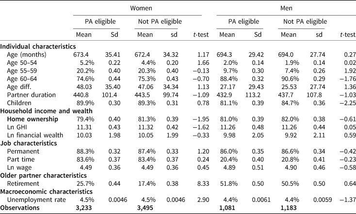
Table 3 shows the descriptive statistics in January 2010 for younger partners whose partner reaches the SPA immediately before or after the reforms. Most younger partners are women (74%) and the majority of them are between 60 and 64 years old when the older partner reaches the SPA. The younger partners in the pre-reform groups are PA eligible (or to be precise, their partners are eligible for the PA), those in the post-reform group are not. Due to the age difference with the older partner, neither group of younger partners is eligible for the generous pre-ER reform early retirement benefits. Differences in characteristics between pre- and post-reform groups are insignificant (according to t-tests with size 0.01) for both sexes, with the exception of the older partner's retirement status (analysed above), particularly for women.
Table 3. Descriptive statistics of younger partners in January 2010
Note: see Table A3 in the Appendix for the definition of the explanatory variables. Age difference and partner duration in months.
Source: Own elaboration from data provided by Statistics Netherlands.
PA eligible and non-eligible groups by gender.
Individuals in the non-PA-eligible group are slightly younger than those in the PA eligible group and men are on average older than women. The average age difference between partners is larger for women (48 months) than for men (27 months) and the average partnership duration is around 36 years for men and women. 90% of the younger female partners and 83% of the younger male partners have children.
Most of the couples (around 80%) own the house where they live. Men exhibit higher household income but lower financial wealth than women do. Similar gender differences in job characteristics are observed for the older partners: Equivalent full-time wages are higher for men than for women. Most of the younger partners had a permanent contract. Among women, 84% had a part-time contract, compared to only 21% of men. The average regional unemployment rate in January 2010 was 4.5%.
Figure 5 shows the transition rates from work into retirement of male and female younger partners by PA eligibility and months until older partner's SPA. Female retirement rates are around 1% until 8 months before the older partner's SPA for both groups, except that for the PA-eligible group, we see peaks at the older partner's ages of 64 (1.8%) and 63 (1.35%), the typical early retirement ages. From 8 months before the older partner's SPA, unlike the PA ineligible group, the eligible group's retirement rates show a jump, and increase more in the month before the older partner's SPA, reaching 6.3%. One month after the older partner reaches SPA, both groups' retirement rates converge again. This suggests that female younger partners are sensitive to the PA, responding to the reform by exiting paid work a few months before their partner's SPA so that they satisfy the conditions for receiving the allowance.

Figure 6. Survival functions. Exits from employment to retirement. Female younger partner and male younger partner by PA eligibility and PA effect. Note: PA eligible (not PA eligible) group: those reaching the SPA before (after) the elimination of the partner allowance. The effect of PA is measured on the right-hand axis. Source: Own elaboration from data provided by Statistics Netherlands.
For the small group of male younger partners (bottom panel of Figure 5), retirement rates show an increasing pattern with age, slightly higher for the PA eligible group. This suggests that male younger partners are not sensitive to the PA. Surprisingly, there is a peak when the older partner reaches age 64 (2.9%) for the non-PA-eligible group.
Figure 6 shows the average survival functions. Unlike older partners, we do not correct for the ER reform effect, since younger partners in both groups (they are at least 2 months younger than older partners) are post early retirement reform. In the female group, the probability that someone has retired at least 1 month before the older partner's SPA is 47% for the PA eligible group and 34.6% for the non-eligible group, suggesting that PA increases the retirement probability for female younger partners by 12.4% points. This difference remains stable for the next year. On the other hand, as we observed in the hazard functions, male younger partners in the non-eligible group show slightly higher survival-in-employment estimates than the PA eligible group. These differences are reduced around the older partner's SPA.

Figure 7. Model 2: Average survival functions in employment, married and singles pre[1]and post-reform. Estimated PA effects and 90% confidence intervals. Males (top panel) and females (bottom panel). Note: Survival functions in employment use the left-hand axis. PA effect (PA; right hand axis) is computed as the difference between the post-reform and pre-reform groups of married and singles. This difference represents the size of the PA disincentive to work. Source: Own elaboration from data provided by Statistics Netherlands.
5. Estimation strategy
To estimate the causal impact of abolishing the PA on the retirement exits of couples, we compared the retirement transitions of couples whose older partner reaches the SPA immediately before (January–February 2015, PA eligible group/pre-reform) and after (March–April 2015, not-PA eligible/post-reform group) the elimination of PA (1 April 2015). We use hazard models since it gives richer modelling possibilities than regression models for the retirement age, as the tendency to retire at specific ages can be taken into account. Moreover, our data are censored 12 months after the older partner's SPA so that the retirement ages of younger partners are often not yet known. Although many studies directly estimate regression models for the retirement age, many other studies also use transition probabilities or probabilities to be in retirement at a given age. See, e.g., Euwals et al. (Reference Euwals, van Vuuren and Wolthoff2010) who emphasize that a hazard rate model has the advantage of accounting for the endogenous selection of those still working at older ages. Kyyrä (Reference Kyyrä2015) also models the transition probabilities out of work. Mastrobuoni (Reference Mastrobuoni2009) models the distance between the survival functions; Laun (Reference Laun2017) and Lalive and Parrotta (Reference Lalive and Parrotta2017) model employment status for each year.
We exploit the cohort variation of the reform as well as the differences in age between partners. We estimate differences between the retirement hazards of PA eligible and not PA eligible groups in which the key variable is the distance (in months) to the older partner's SPA. If no other reforms affect either group, differences in the outcomes can be attributed to the eligibility to the PA. This is definitely not the case for the older partners: Those in the non-PA-eligible group also suffered the reduction in early retirement benefit opportunities, due to the ER reform. Since younger partners, due to the age difference, are always in the post-ER-reform group, such correction does not seem necessary to estimate the effect of the PA reform for younger partners.
To account for the effect of the ER reform in the analysis for older partners, we use difference-in-differences, comparing with the single individuals who are always ineligible to PA but are affected by the early retirement reform. This is based upon the identifying assumption that the effect of the ER reform is the same for married and single individuals. This assumption is justified in several earlier studies (Baker, Reference Baker2002, p18; Atalay and Barrett, Reference Atalay and Barrett2016). For the Netherlands, Euwals et al. (Reference Euwals, van Vuuren and Wolthoff2010) analysed the causal impact of the early retirement reforms that took place in the early 1990s on retirement, exploiting variation in the dates of the reform. They found no significant difference in the effects of the ER reforms between single and married individuals. Bloemen (Reference Bloemen2011) found no effect of marital status on the retirement rate of Dutch male elderly workers in the period 1995–2002. The similarity of the patterns for singles and older partners in couples in Figure 3 also supports this assumption.
We cannot test the common pre-reform trend assumption since our data only cover a short pre-reform period. In Section 7, we discuss some threats to our identifying assumptions and provide more evidence suggesting their validity.
5.1 Transitions from work to retirement
We model the transitions out of work into retirement using a discrete-time proportional hazard model with a logit functional form:

Here Y it = 1 if individual i is retired at age t (in months) and Y it = 0 if the individual is working.
The model is estimated using maximum likelihood. Given that the model is non-linear, we compute the average marginal effects (AMEs) for different specifications. We estimate the model separately for older and younger partners and by gender.
5.1.1 Older partners
Our most extensive specification is

Here h 0(t) is a non-parametric baseline hazard (with monthly dummies). The model includes
1. The ‘Post-reform’ dummy T i = 1{birthday i > Dec1949} (1 if the individual is born in January or February 1950, and 0 if born in November or December 1949).
2. The ‘dummy married’ (1 if the individual is married or in a registered partnership; 0 if single, divorced, separated, or widowed).
3. The Diff-in-Diff term: the interaction of married and post-reform dummies, capturing the effect of abolishing the PA (our main parameter of interest).
4. In our most complex specification, we interact the Diff-in-Diff term with time dummies to explore how the effect of the PA reform varies with time to SPA.
The vector P i contains personal characteristics; those specific for couples are set to 0 for single individuals. We control for the state of the economy using the regional unemployment rate (u_rate). The vector $W_{it_0}$ is a vector of initial conditions, including gross household income, financial wealth quartile and homeownership measured at the beginning of the observation period. Finally, the vector $J^{\prime}_{i, t-1}$
 includes (lagged) job characteristics, such as wages and dummies for permanent and part-time contracts.Footnote 18
5.1.2 Younger partners
Unlike older partners, both groups of younger partners (pre-PA-reform and post-PA-reform) are affected by the ER reform, so that it is sufficient to consider the single difference rather than applying difference-in-differences.
We assume that the probability that younger partner i transits from work to retirement between times-to-older-partner's-SPA t and t + 1 is driven by the following equation:

As in equation (2), h 0(t) is the non-parametric baseline hazard with monthly time dummies, capturing the pattern of the retirement rate by distance to the older partner's SPA (from 59 months before to 12 months after the older partner's SPA).
The key variable ‘No-PA’ dummy T i = 1{ older partner's birthdayi > Dec1949} takes value 1 if the older partner reaches the SPA in April or May 2015 (just after the elimination of the PA), and 0 if the older partner reaches the SPA in February or March 2015. Like for older partners, in the simplest model (Model 1) there is one treatment effect that remains constant over time. In the most extensive specification, we also interact T i with the monthly time dummies, allowing the effect of PA to vary with time to the partner's date of reaching SPA.
As for older partners, we include the vectors P i, $W^{\prime}_{it_0}$ , and $J^{\prime}_i$
 and control for the state of the economy. Unlike the model for older partners, the individual's age (in months) is included in a quadratic form, as well as a control for the lagged retirement status of the older partner (ret_op_it−1; taking the lag avoids endogeneity issues). We also interact the latter with the post-reform (No-PA) dummy.
6. Estimation results
6.1 Older partners
We estimate the probability to exit from work into retirement for older partners by gender using four different specifications. Results are presented in Table 4.Footnote 19 Model 1 includes the post-reform dummy, the dummy married, and the interaction of these two (the DiD term); in addition, it includes personal characteristics (gender, age difference between spouses, partner duration, children) and the regional unemployment rate. In Model 2, we add the interactions of the DiD term with the dummies for distance (in months) to the SPA. Model 3 is similar to Model 2 but adds some initial conditions (homeownership, financial wealth, and household incomes). Model 4 adds previous job characteristics (permanent contract, part-time contract, and wages) to Model 3.
Table 4. Estimation results of the logit model for older partners and singles (exit from work into retirement)

Note: Standard errors clustered by individual in parentheses.
‘PA effect’ is the difference between the average marginal effects of the post-reform dummy for married and singles.
Older partners and singles reaching SPA before and after 1 April 2015.
*p < 0.05; **p < 0.01; ***p < 0.001.
6.1.1 Effects of PA eligibility on retirement
In Table 4, the DiD coefficient in Model 1 reflects the effect of the PA reform on the older partner's retirement probability in the 59 months before the older partner reaches the SPA until 6 months after. The negative and significant (at the 5% level) value for men implies that not being eligible to the PA reduces the probability to go from paid work into retirement. The AME is a 0.16 percentage points reduction in the monthly exit probability. An effect of similar size (−0.18 percentage points) is found for women but this is insignificant, due to the much smaller sample size for older female partners.
As a sensitivity check, we also estimated Model 1 for a more restricted sample where the age difference between partners is at most 5 years instead of 10 years (417,317 observations for men, 201,373 for women). The estimated PA effects are similar to those using the complete sample: 0.177 percentage points (s.e.: 0.095) for men, −0.170 percentage points (s.e.: 0.150) for women.
Moreover, we added eight dummies for the sector of activity of the older partner, since retirement behaviour might differ by sector. This hardly changes the main results: the estimated PA effects are 0.15 pp for men (s.e.: 0.092) and 0.22 pp for women (s.e. 0.130).Footnote 20
Model 2 allows the effects to be different each month. The AMEs are similar. Instead of presenting all the coefficients, we illustrate the implications of Model 2 estimates in Figure 7 (males in the top panel, females in the bottom panel). The figure presents the estimated survival functions (the probabilities to remain employed; left-hand axis) for the four groups (older partners and singles pre- and post-reform) and the DiD estimates of the effect of the PA reform on the probability to remain employed (right-hand axis), as well as the 90% confidence bands for the latter.
As expected, post-reform groups show higher survival probabilities in employment and the differences between pre-and post-reform groups are higher for the older partners group than for the singles. The difference is our estimate of the effect of the PA reform, affecting only the older partners and not the singles group (‘PA’ in the figure). For male older partners, the effect is already present about 4 years before they reach SPA, and it slightly increases until reaching SPA. The PA reform increases their probability to remain in employment at ages between 61 and 65 by about 2 to 3 percentage points on average. For example, PA eligibility increased the probability of being retired before age 63 by 2.3 percentage points. The confidence intervals indicate that some of the effects are significant at the two-sided 10% level. For female older partners, the effects start somewhat later and are even somewhat larger (2.7 percentage points at age 63), but the estimates are also less precise, due to the smaller size of the sample.
6.1.2 Covariates
Model 3 adds some explanatory variables on the household's initial financial and housing wealth (5 years before the older partner reaches SPA). Adding these variables hardly affects the estimates of the reform effects, but is of some interest by itself. They show that older partners in the higher financial wealth quartiles tend to retire earlier. This is in line with a positive income effect on early retirement: individuals retire early if they can afford it. For men, the probability to go into retirement is lower if the age difference with the younger partner is larger. Male older partners in longer relationships have a higher probability of retirement. Having children has a negative and significant effect on retirement for both sexes, probably since individuals and couples help their children financially or have a bequest motive. Men and women living in regions with higher unemployment rates have a higher probability of retirement.
The results on financial and housing wealth change, however, if we also control for lagged job characteristics and household income (Model 4). The effects of financial wealth are much smaller and no longer significant for women. Instead, lagged earnings play a dominant role: the individuals with the higher wages (and, probably, the higher occupational pensions) can afford to retire early. Moreover, individuals working part-time retire earlier, perhaps since their link to the labour market is less strong already. Homeownership has a significantly negative effect, possibly because many owners still have to redeem their mortgage. Surprisingly, gross household income is significantly negative for retirement. Men with a permanent contract are more likely to retire, possibly because they are entitled to a larger occupational pension.
6.2 Younger partners
To estimate the (causal) effect of the PA on the younger partners´ probability of retirement, we estimate six different specifications separately by gender. Complete estimation results are presented in Table 5. Model 1 includes the dummy of interest, ‘No-PA’ (1 if the older partner reaches the SPA after March 2015 and is not entitled to the PA, 0 otherwise), personal characteristics (gender, age in a quadratic form, age difference between spouses, partner duration, and children) and the regional unemployment rate. In Model 2, in the spirit with the most complex model for older partners, we add the interactions of the No-PA dummy with the time dummies of the distance (in months) to the older partner's SPA, capturing time-varying treatment effects. The other models maintain this. Model 3 adds initial conditions (homeownership, financial wealth, and household incomes) to Model 2. Model 4 adds lagged characteristics of the job (permanent contract, part-time contract, and wages), but excludes household incomes. Model 5 adds the previous retirement state of the partner. Model 6 includes the interaction of the partner´s previous retirement state and the No-PA dummy. Lastly, we extend Model 1 adding the interaction of the part-time dummy and the ‘No-PA’ dummy.
Table 5. Estimation results of the logit model for younger partners (exit from work to retirement)

Note: Standard errors clustered by individual in parentheses.
Male (top panel) and female (bottom panel) younger partners. Models 1–6.
*p > 0.05; **p < 0.01; ***p < 0.001.
6.2.1 Effects of being entitled to the PA on retirement
We first test if there is any significant response of the younger partners to the PA eligibility. The estimated AMEs of No-PA (post-reform) on retirement are shown in Table 6. The negative and significant AMEs of the PA reform on the female´s retirement hazard (a reduction in the monthly retirement probability of about 0.26 to 0.29 percentage points) suggest that, as expected, PA eligibility is an incentive to stop working for female younger partners. In contrast, AMEs are small and insignificant for men, suggesting that male younger partners are not responsive to PA.
Table 6. Average marginal effects of PA reform on the monthly probability to retire for younger partners

Note: No PA: older partner reaches the SPA after PA is abolished. Standard errors clustered by an individual in parentheses.
*p < 0.05; **p < 0.01; ***p < 0.001.
To explore if differences in the response to the PA incentive between men and women exist for full-time and part-time workers, we estimate AMEs of the PA reform on the probability to retire in an extension of Model 1 which includes an interaction of the treatment effect with the part-time dummy. According to the results in Table 7, male and female full-time workers and male part-time workers (20% of male younger partners doing paid work) do not respond significantly to the PA incentive. In contrast, female part-time workers (83% of female younger partners doing paid work) do respond by reducing their labour supply. The aforementioned differences are therefore due to the response of part-time workers.
Table 7. Average marginal effects of PA reform on the monthly probability to retire for younger partners; full-time and part-time workers

Note: Standard errors clustered by individual in parentheses.
Extended Model 1.
*p < 0.05; **p < 0.01; ***p < 0.001.
The reason for the difference might be the relative importance of the financial incentive compared to the loss in earnings. The PA is a fixed amount, but retiring typically involves a much larger earnings loss for full-timers than for part-time workers.Footnote 21
For Model 2, Figure 8 illustrates the impact of the PA reform on the probability to remain in employment by comparing the average survival probability in work of the PA-eligible and non-PA-eligible groups. For male younger partners, the difference between the pre- and post-reform groups is small at any point in time, with slightly higher probabilities to stay in employment for the post-reform group, in line with the small negative estimates in Table 6. It confirms that male younger partners hardly respond to the reform.

Figure 8. Model 2: Average survival functions in work by PA eligibility and effects of PA with 90% confidence intervals for younger partners, from 60 months before until 12 months after the older partner reaches SPA. Females (top panel) and males (bottom panel). Note: Survival functions in employment use the left-hand axis. PA effect (PA; right-hand axis) is computed as the difference between the post- and pre-reform groups. Source: Own elaboration using data from Statistics Netherlands.
For female younger partners in the pre-reform group, we see a substantial jump in the probability to be retired in the period just before the partner reaches SPA. This is the effect of the PA, creating an incentive for the younger partner to stop working before the older partner reaches the SPA. As a result, the probability to work when the older partner reaches the SPA is 55.8% before the reform and 67.2% after the reform. This difference remains stable and significant over the next 12 months. The large effect is in line with the simulation analysis of Mastrogiacomo et al. (Reference Mastrogiacomo, Alessie and Lindeboom2004).
6.2.2 Covariates
Focusing on Table 5, for most of the age range, age has a negative effect on the retirement hazard. It becomes positive after age 66 (males) or 67 (females). Surprisingly, the larger the age difference with the older partner the higher the probability to retire. Having children is associated with a lower probability to retirement, but it is not significant once wealth and income controls are included (Models 3 to 6). Homeownership is positively associated with females' retirement but only significant in Model 3; it is insignificant for males. Household income is negatively associated with retirement for both men and women.
According to Model 3, the richer (in terms of financial wealth) the younger partner, the more likely he or she is to retire. After controlling for lagged job characteristics, however, financial wealth is no longer significant. Similar to the results for older partners, high wage earners are those who (can afford to) retire early. Having children has a negative and significant effect on retirement for both sexes. Men and women living in regions with higher unemployment rates have a higher probability of retirement. Having a permanent contract has a significant negative effect on retirement for women. Part-time has a positive and significant effect on the probability to retirement, particularly for men. Finally, having a retired older partner increases the probability of retirement, possibly pointing at complementarities in leisure – the retirement of the partner increases the marginal utility of leisure since there is more time for joint leisure activities (cf., e.g., Stancanelli and van Soest, Reference Stancanelli and van Soest2016). This effect is stronger, in relative terms, for men than for women.
6.3 Comparison to existing findings
Online Appendix Table OA2 summarizes the results of a number of existing studies on pension reforms. The nature of the reforms and the outcome measures vary substantially across studies, making it hard to directly compare the results. The largest reform effect we find is for female younger partners (an increase of approximately 11 percentage points in the probability to remain employed shortly before the older partner reaches the SPA). Mastrogiacomo et al. (Reference Mastrogiacomo, Alessie and Lindeboom2004) analyse a somewhat comparable reform in the Netherlands, but with a much smaller change in the rewards to working longer. The effect that we find seems much larger than the effect found by Mastrogiacomo et al. (Reference Mastrogiacomo, Alessie and Lindeboom2004), even if we account for the smaller change in rewards. The spouse allowance analysed by Baker (Reference Baker2002) also reduced the rewards for working. The effect he found for males and females (7 percentage points and 4 to 9 percentage points, respectively) are in the same range as what we find for females. Euwals et al. (Reference Euwals, van Vuuren and Wolthoff2010) analysed a reform that rigorously changed the rewards to working during the years before the standard retirement age for many individuals. The substitution effect of an eight months increase in the average retirement age seems large compared to what we find – if the 11% that remain employed work until their own SPA, we would get an increase of about four or five months in the average retirement age for younger female partners. This also seems small compared to Brown (Reference Brown2013) who finds an increase of about 6 months in response to a much smaller change in the rewards to working. Interpreting the PA as early access to a state pension, we can also compare the effect to studies that consider the effect of changing the threshold for early retirement benefits. Compared to these studies, the effect we find is small. For example, Kyyrä (Reference Kyyrä2015) finds that access to an early old-age pension increases the odds of non-participation by 193% for women and by 49% for men.
We interpret the effect on the older partner as mainly an income effect, although it could also be an indirect effect of the change for the younger partner, e.g., due to complementarities of leisure. We find that the reform increased participation in paid work by between 2 and 3 percentage points. Given the size of the income change, this seems a modest effect compared to studies like Gurley-Calvez and Hill (Reference Gurley-Calvez and Hill2011), Bloemen et al. (Reference Bloemen, Hochguertel and Zweerink2019), Mastrobuoni (Reference Mastrobuoni2009) or Atalay and Barrett (Reference Atalay and Barrett2015). In the latter two cases, the difference might be related to the fact that their reforms also changed the standard retirement age, possibly inducing a large behavioural effect through the social norm or reference point (Behagel and Blau, Reference Behagel and Blau2012). On the other hand, Lalive and Parrotta (Reference Lalive and Parrotta2017) find effects of pension eligibility of the male spouse on the labour supply of the other spouse of a similar order of magnitude as the effects that we find, and Laun (Reference Laun2017) finds no significant effect of reform in tax credits for one partner on the participation of the spouse.
7. Spill-over effects and the validity of the identifying assumptions
Our main identifying assumption needed to estimate the effect of the PA reform on older partners' labour supply in Sections 5 and 6 was that the effect of the ER reform is the same for singles and individuals in couples. Previous empirical evidence supports this assumption: Euwals et al. (Reference Euwals, van Vuuren and Wolthoff2010) analysed the impact of the early retirement reforms that took place in the early 1990s on retirement behaviour in the Netherlands and found no significant effects of marital status on the effects of the ER reforms on the retirement behaviour.
On the other hand, this assumption may be invalid if there are indirect (multiplier) effects through the partner, as illustrated in Table 8. The ER reform may have a spill-over effect on the younger partner. If the younger partner changes their retirement or labour supply decision, this may in turn affect the labour supply decision of the older partner.
Table 8. Direct and indirect effects of the reforms for singles and older and younger partners by spouse's labour market attachment

Note: ‘ON’: Older partner with a younger partner not – attached to the labour market; ‘OA’: Older partner with a younger partner attached to the labour market; ‘YN’: Younger partner with an older partner not attached to the labour market; ‘YA’: Younger partner with an older partner attached to the labour market.
Source: Own elaboration.
To investigate whether such indirect effects play a role, we estimate the model for older partners separately for the subsamples where the younger partner is (initially) attached to the labour market or not. Indirect effects can be expected if the younger partner is attached to the labour market, but not if he or she does not supply any labour anyhow. A substantial difference in the effects on older partners between those with an attached and non-attached partner would imply that indirect effects are important, invalidating our identifying assumption.
Similarly, in Section 6 we have estimated the effects of the PA reform on younger partners for the combined sample with older partners attached and not attached to the labour market. If indirect effects play a substantial role, the total effect of the PA reform on younger partners will be different depending on whether the older partner is or is not attached to the labour market, since the indirect effect can only occur in the former case. We therefore also estimate the model for younger partner separately for the cases where the partner is or is not attached to the labour market.
To define whether an individual is attached to the labour market or not, we consider their initial labour market status, five years before the older partner reaches the SP eligibility age.Footnote 22 This gives, for males and females, five subsamples, each consisting of pre- and post-reform groups: Singles (S), older partners with partner attached (OA) or not attached (ON) to the labour market, and younger partners with partner attached (YA) or not attached (YN) to the labour market. We will estimate separate reform effects for these subsamples.
First, online Appendix Table OA3 checks the similarity in sample characteristics between pre-reform and post-reform subgroups in each of the subsamples. It shows that, according to 1% level t-tests, differences between the two groups are not significant with only one exception – children for the (rather small) subsample of single men.
In Table 9, we present the estimated AMEs of the PA reform using the extension of Model 1 in the previous section with an interaction term of partner's labour market attachment and post-reform dummy to allow for different effects depending on the labour market attachment of the partner. In line with our main results, we find that the reform reduces the hazards to retire. As before, female younger partners are more responsive than male younger partners, irrespective of the partner's labour market attachment. For older partners, we again find the reverse: larger and more significant effects for males than for females.
Table 9. Average marginal effects of PA reform on retirement by partner's labour market attachment

Note: Standard errors clustered at the individual level in parentheses.
Model 1.
*p < 0.05; **p < 0.01; ***p < 0.001.
The only notable difference between the cases where the partner is or is not attached to the labour market is found for female older partners. In this case, the PA reform effect is larger if the male younger partner is attached to the labour market than if he is not, and significant in the first case only. The difference is not significant, however, so even in this case, there is not enough evidence to conclude that attachment of the partner matters. The results show that the differences between spouses with partners attached and non-attached are small and insignificant for both genders in all other cases. Model 2 (not shown) gives the same results. These results imply that indirect effects do not play a significant role, supporting our identifying assumptions.
7.1 Placebo test
We test whether observed differences between pre- and post-reform groups are indeed due to the elimination of the PA and the early retirement reform using a ‘placebo test’. We estimate the retirement hazards for similar groups but reaching their SPA in February–March 2014 and April–May 2014, one year before the reform.Footnote 23
For the older partners, online Appendix Figure OA2 shows the probability to be working rather than retired (the survival function) by gender from the raw data. As expected, for both men and women, the survival functions are similar for pre and post 1 April 2014 groups. In line with this, the AMEs of the policy reforms on retirement are never significantly different from zero; see online Appendix Table OA3.
The average survival estimates for younger partners are displayed in online Appendix Figure OA2. Survival estimates for the two groups of women are almost identical. Men in the pre-1 April 2014 group show a slightly larger probability of retirement than those in the post-1 April 2014 group. However, the AME of the effects on retirement is never significantly different from zero (online Appendix Table OA4). All in all, the similarity of the retirement hazards for the pre- and post-1 April 2004 groups confirms that the effects we found for 2015 are indeed due to the reforms that took place in that year.
7.2 Heterogeneous effects
Couples whose younger spouse has high initial earnings may be less impacted by the reform, as their PA amount is relatively small compared to the younger partner's wage.Footnote 24 We therefore estimated Model 1 for couples whose younger partner works 5 years before the older partner reaches their SPA, adding the interaction of the post-reform dummy and the dummy ‘wage 5 years before older partner's SPA above the median’. Indeed, we find that the AME of the reforms on the older partner‘s participation (PA plus ER) for the low wage group is larger than for the high wage group, but the differences are small and insignificant for both males and females. Similar results are obtained when four wage quartiles are distinguished (see online Appendix Tables OA5 and OA6).
The magnitude of the income effect on the older partner's retirement decision may also increase with the number of years PA applies, i.e., the age difference between spouses – if the younger spouse does not participate, the life-cycle income difference is linearly increasing with the age difference. To investigate this empirically, we estimated Model 1 adding an interaction term of the reform effect with the age difference (see online Appendix Tables OA7 and OA8). The estimates show a larger negative effect of the reform for a larger age difference, as expected, but the interaction term was insignificant for both male and female older partners (with t-value less than 1). For younger partners, the reform effect also increases with the age difference, and the interaction is marginally significant (at the 5% level) for women but not for men.
The estimates for younger partners suggest that the PA effect is about 1.5 times as large for the maximum age difference (5 years) than for the minimum difference (3 months). Since the younger spouse must have low earnings at the time the older spouse reaches SPA, a larger age difference requires leaving work at an earlier age for the younger spouse. Indeed, the number of years a couple benefits from PA increases linearly with the age difference between the two spouses. This affects the total benefits the couple can get, but also the costs in the form of foregone earnings of the younger spouse. It is therefore not clear a priori whether the PA reform has a larger effect when the age difference is larger.
8. Conclusions
In this study, we have analysed the effect of eligibility to the PA on the retirement of couples in the Netherlands. PA was a supplementary allowance to the state pension paid to the partner who already reached the state pension eligibility age (SPA), conditional on zero or low earnings of the younger partner. This allowance created financial incentives possibly affecting the labour supply of both partners in the couple via substitution and income (or lifetime wealth) effects.
To quantify the causal effect of PA eligibility on both spouses’ retirement probabilities, we exploit the elimination of PA in 2015. For older partners, to account for the fact that the same birth cohorts of older partners are affected by a reform in early retirement benefits (the ER reform), we use a difference-in-differences identification strategy, assuming that the ER reform had the same effect on single individuals and individuals in couple. For younger partners, we do not need this assumption or a DiD strategy, since they are all from post-ER-reform cohorts. This makes the analysis for younger partners more straightforward and more convincing.
We compared the retirement probabilities of narrowly defined groups affected and not affected by the reforms. We quantify the accumulated effects of PA on the probability to be retired as the difference of the average survival probability in employment between the pre- and post-reform groups, correcting for the effect of the ER reform for the older partners.
For the older partners, our findings point to a small incentive role of PA on early retirement. For example, PA eligibility increases the probability to retire before reaching age 63 (65) by 2.3 (3.5) percentage points for men and by 2.7 (2.6) percentage points for women. Since the effects are similar for the cases where the partner is or is not attached to the labour market some years earlier, this finding points at the importance of pension wealth shocks for retirement decisions (‘income effects’) rather than at joint retirement considerations. The symmetry of the cross-effects is remarkable compared to the existing literature. The largest peak (before the SPA) in the retirement hazard and the largest effect of PA eligibility is found at the former state pension age of exactly 65 years, 3 months before the state pension age at the time of the reform. The large retirement hazards at this age are probably explained by a social norm or age anchor since 65 years was the SP age and the common mandatory retirement age for many years. After the reform, many individuals could no longer afford this form of early retirement, reducing the effect of anchoring or social norms.
For younger partners, the design of the PA – means-tested on the younger partner's income – created a direct incentive to stop working – a substitution effect. In addition, wealth and joint retirement effects could affect the younger partner's retirement decisions. We find no significant effects for male younger partners, either working full-time or working part-time. Female younger partners responded significantly, particularly if they worked part-time (the majority of female workers in the Netherlands). The PA increased the probability of going into retirement at least 6 months before the older partner's SPA by 11 percentage points. Following the arguments of Selin (Reference Selin2017), the difference between men and women might be due to the fact that age anchors or reference points play a larger role for men than for women, as suggested by the large retirement rate for men at age 65. The PA effect starts approximately 6 months before the older partner's SPA and reaches its highest value (5 percentage points) in the month before the older partner's SPA.
Our results are relevant for the policy design of pension reforms and for forecasting the fiscal impact of the reform. The asymmetric effect for younger partners has implications for the gender gap in labour force participation of older age groups and, as a consequence, for the gender gap in pension adequacy. Moreover, significant spill-over effects on the spouse need to be accounted for when evaluating a retirement policy reform.
Supplementary material
The supplementary material for this article can be found at https://doi.org/10.1017/S1474747221000299.
Acknowledgements
The authors thank the editor Courtney Coile, two anonymous reviewers, Jochem de Bresser, Hans Bloemen, Egbert Jongen, and other participants in the Netspar Pension Day 2018, the International Pension Workshop 2019 and seminars at IZA, the University of Gerona and CPB.
Appendix
Table A1. Evolution of the SPA 2008–2018

Table A2. State Pension amounts by partnership status (July 2016)

Table A3. Definition of the explanatory variables


 Open access