


1. Introduction
The USA has long incentivized retirement saving by deferring taxes on workers' pension contributions until the assets are withdrawn in old age, at which point the withdrawn funds become subject to income tax. In this way, most of the $25 trillion nest eggs that workers hold in employer-sponsored defined contribution 401(k) plans and individual retirement accounts (IRAs) are taxed according to an ‘Exempt-Exempt-Taxed’ (EET) regime (ICI 2021)Footnote 1: workers contribute out of pre-tax earnings, recognize pre-tax investment earnings in their accounts, and pay income tax on withdrawals during retirement. This policy has a large current fiscal cost: some estimates claim that the US Treasury foregoes over $100 billion per year due to tax-deferred contributions to 401(k) and similar plans (Thornton, Reference Thornton2017).Footnote 2
Partly because of current and projected federal budget shortfalls, some policymakers have proposed eliminating or capping tax-qualified retirement plan contributions, a practice termed ‘Rothification’, named after Senator William Roth who, in 1997, sponsored legislation permitting this. The Rothification idea has been a topic of considerable recent discussion, with former President Obama recommending a pre-tax pension contribution cap in 2015; related proposals were mooted during the 2017 tax reform debate (Schoeff, Reference Schoeff2017). Though those proposals were not enacted, the topic is certain to be revisited given the amount of revenue involved and the size of the ballooning fiscal deficit. In addition to analyzing the effect on the fiscal cost of changing tax incentives to promote retirement savings, it is of key importance to assess the potential impact on household behavior. This is because if such a reform were to be passed, it could have important behavioral implications with effects that could vary across population subgroups.
This paper investigates the potential impact of treating all future retirement contributions to a ‘Taxed-Exempt-Exempt’ (TEE) regime, in which workers contribute to their pensions out of after-tax income with no additional tax on investment earnings, and withdrawals would be levied thereafter. In an economy without uncertainty, a single proportional tax rate on a household's entire income, the absence of borrowing constraints, and where savings are contributed out of after-tax income versus later in retirement would not change household behavior (Feldstein, Reference Feldstein1969; Burman et al., Reference Burman, Gale and Weiner2001). In reality, of course, households are exposed to considerable uncertainty over their lifecycles due to stochastic mortality, health shocks, capital market volatility, and labor income risks. In addition, the US tax system is progressive, imposes different tax rates on different income sources, and embeds numerous nonlinearities. This applies, in particular, to the tax treatment of pension schemes.Footnote 3 For example, there are tax-relevant upper and lower limits for contributions into and withdrawals from private or employer-sponsored pension plans. Non-compliance with these limits can attract income taxes and additionally lead to severe tax penalties. Furthermore, tax incentives for funded pension schemes such as 401(k)s with voluntary participation cannot be considered in isolation from the national mandatory retirement system. Social Security taxes are levied in proportion to labor income, but only up to a maximum threshold. Social Security retirement benefits are calculated as a non-linear (concave) function of average lifetime earnings and are only partially included in taxable income, again according to a non-linear formula (on combined income). Moreover, the US Social Security system includes complex financial incentives to encourage delayed benefit claiming. As the literature shows (Shoven and Slavov, Reference Shoven and Slavov2014; Hubener et al., Reference Hubener, Maurer and Mitchell2016), when to exercise this option also depends on financial assets accumulated for retirement.
In a world with uncertainty and where taxes and benefit are highly non-linear, it is less obvious how implementing a move from EET to TEE taxation of funded pension plans would alter household behavior. Specifically, it requires modeling the rich institutional details confronting real-world consumers along with their economic environment, capital and labor market risk, and uncertain lifetimes. Previous research including Dammon et al. (Reference Dammon, Spatt and Zhang2004), Gomes et al. (Reference Gomes, Michaelides and Polkovnichenko2009), Poterba (Reference Poterba2004), and Shoven and Sialm (Reference Shoven and Sialm2003), studied the effect of tax-qualified retirement accounts on savings and portfolio decisions for households maximizing lifetime consumption utility, but those studies used the classical EET framework and omitted work and retirement decisions. A recent empirical study by Beshears et al. (Reference Beshears, Choi, Laibson and Madrian2017) documented that adding a Roth contribution option to existing traditional tax-deferred 401(k) plans would not change saving rates, under some circumstances. A simulation study by OECD (2018) provided a theoretical analysis of the EET versus TEE approach; nevertheless, the metric used by the OECD to compare the two tax regimes – the overall lifetime tax advantage – did not incorporate household behavioral responses to changes in tax incentives. Lachance (Reference Lachance2013) compared investor decisions between a traditional tax-qualified retirement account versus a Roth account, but she did not incorporate Social Security claiming behavior, endogenous work hours, risky labor income, or market return risk, as we do here. Brown et al. (Reference Brown, Cederburg and O'Doherty2017a, Reference Brown, Poterba and Richardson2017b) found that there is some uncertainty in future income tax rates, so Roth accounts could be an important vehicle to mitigate the risk resulting uncertainty over future tax schedules.
We add to the literature by delving into possible consequences of such a reform on household behavior in the context of a richly detailed state-of-the-art life-cycle model. This model allows us to analyze of how Rothification could alter utility-maximizing households' consumption and work patterns, taking into account labor income risk, investments in risky stocks and bonds inside/outside retirement accounts, Social Security claiming patterns, and tax payments. The model also incorporates realistic Social Security contribution structures and benefit formulas including adjustments for early and delayed claiming. Furthermore, our model includes US federal/state income tax and real-world rules characterizing tax-qualified 401(k) accounts, including caps on 401(k) pre-tax contributions and employer matches, as well as penalty taxes on non-qualified early distributions, and required minimum distribution (RMD) withdrawal amounts. Of key importance is ex ante heterogeneity: workers out the outset face different educational and mortality profiles, as well as ex post heterogeneity, due to labor income and capital return risk. To this end, we measure how key outcomes differ across several worker-types differentiated by sex and education, since some have argued that ‘Roths may not, in fact, work out to be a better deal’ for low-income people (Tergesen, Reference Tergesen2017).Footnote 4
It is additionally important to recognize that converting retirement accounts to Roth plans will take place against the backdrop of the income tax structure introduced in 2018, which reduced the tax burden for most earners.Footnote 5 That reform changed the relative attractiveness of saving for retirement in an EET environment, since lower marginal tax rates on workers' earnings reduced the attractiveness of saving in 401(k) accounts. Accordingly, our research compares how work, saving, benefit claiming behavior, and tax payments differ in an EET versus TEE setting, for a variety of heterogeneous workers.
In what follows, we first build and calibrate a structural life-cycle model assuming an EET framework. Results agree closely with observed consumption, saving, and Social Security claiming patterns of US households, while matching the distribution of 401(k) wealth rather nicely. Next, we develop results under an alternative environment where 401(k) contributions are taxed according to a TEE structure. This permits us to identify differences in behavior for the heterogeneous workers described above, under both tax regimes (EET versus TEE). Specifically, we assess whether the lower-paid behave differently from the higher-paid in terms of savings inside and outside tax-qualified accounts, as well as in non-pension savings accounts, and whether they would change their Social Security claiming ages. In addition, we are interested in how Rothification would alter the distribution of retirement outcomes relative to the current EET system. For example, the gap between high- and low-wage workers' take home pay is not diminished by income taxes under an EET system, whereas it is under a TEE program. Moreover, the Social Security replacement rate formula is concave, as it provides relatively higher benefits for low-wage workers than for the higher paid. Given this, an EET scheme enhances the progressivity of overall old age income (pension account withdrawals plus Social Security benefits), whereas a TEE structure treats retirement benefits more neutrally. Finally, we compare expected household tax payments over the lifecycle under both the EET and TEE regimes.
2. Consumer's life-cycle problem: model and calibration
This research builds on prior work (Horneff et al., Reference Horneff, Maurer and Mitchell2019) by exploring the impact of a Rothification reform for 401(k) plans, while accounting for the current US income US tax regime. Our contribution is to develop a structural dynamic consumption and portfolio choice model for an individual maximizing his lifetime utility over consumption and leisure, using a richly specified, sophisticated formulation of lifetime behavior calibrated to US federal/state income tax and Social Security/Medicare premium structures, along with realistic Social Security benefit formulas.Footnote 6
2.1 Preferences
We work in discrete yearly time steps and assume that the worker's decision period starts at t = 1 (age 25) and ends at T = 76 (age 100). The household has an uncertain lifetime, such that the probability to survive from t until the next year t + 1 is denoted by p t. Survival rates entering into the utility function are taken from the US Population Life Table (Arias, Reference Arias2010). Preferences are represented by a Cobb Douglas function $u_t( {C_t, \;l_t} ) = ( {{( {C_tl_t^\alpha } ) }^{1-\rho }/( 1-\rho ) } )$ based on current consumption C t and leisure time lt (normalized as a fraction of total available time). The parameter α measures leisure preferences; ρ is the coefficient of relative risk aversion; and β is the time preference factor. The recursive definition of the value function is given by:

with terminal utility $J_T = ( {{( {C_Tl_T^\alpha } ) }^{1-\rho }/( 1-\rho ) } )$ and l t = 1 after retirement. We calibrate the preference parameters so our results match empirical claiming rates reported by the US Social Security Administration and average assets in tax-qualified retirement plans in the EET setting (for details, see below).
2.2 Time budget, labor income, and Social Security retirement benefits
As in Horneff et al. (Reference Horneff, Maurer and Mitchell2019), our model allows for flexible work effort and retirement ages. The worker allocates up to (1 − l t) = 0.6 of his available time budget to paid work (assuming 100 waking hours per week and 52 weeks per year). Depending on his work effort, the uncertain yearly before-tax labor income is given by:

Here, w t is a deterministic wage rate component which depends on age, education, sex, and an indicator for whether the individual works full time, part time, or overtime. The variable P t+1 = P t ⋅ N t+1 is the permanent component of wage rates with independent lognormal distributed shocks $N_t\sim LN( {-0.5\sigma_P^2 , \;\;\sigma_P^2 } )$ having a mean of one and volatility of $\sigma _P^2$
 . In addition, $U_t\sim LN( {-0.5\sigma_U^2 , \;\;\sigma_U^2 } )$
 is a transitory shock with volatility $\sigma _U^2$
 and assumed uncorrelated with N t.
The calibration of the deterministic component of the wage rate process $w_t^i$ and the variances of the permanent and transitory wage shocks $N_t^i$
 and $U_t^i$
 is based on data from Panel Study of Income Dynamics. We estimate these separately by sex and educational level, where the latter groupings are less than High School, High School graduate, and at least some college (<HS, HS, Coll+; see Appendix A, Table A1).
Between the ages of 62 and 70, a worker may retire from work and claim Social Security benefits. The benefit formula is an overall concave piece-wise linear function of the worker's average indexed lifetime earnings. This formula generates an annual unreduced Social Security benefit – called the primary insurance amount (PIA) – equal to 90% of (12 times) the first $895 of average indexed monthly earnings, plus 32% of average indexed monthly earnings over $895 and through $5,397, plus 15% of average indexed monthly earnings over $5,397 and up to the cap $10,700 (in 2018).Footnote 7 Should an individual claim benefits before (after) his system-defined Normal Retirement Age of 66, his lifelong Social Security benefits are permanently reduced (increased) according to pre-specified factors. If an individual works beyond age 62, the model stipulates that he devote at least 1 hour per week; also, our model rules out overtime work in retirement (i.e., 0.01 ≤ (1 − l t) ≤ 0.4).
2.3 Taxation and evolution of retirement plans
During the worklife and in retirement, households must pay various taxes (Tax t+1) which reduce cash on hand available for consumption and investment. The amount and timing of these tax payments over the lifecycle differ significantly in the case of an EET versus TEE system.
First, workers must pay payroll taxes $PT_{t + 1}^{tax}$ amounting to 11.65%, which is the sum of 1.45% Medicare, 4% city and state tax and 6.2% Social Security tax (up to a maximum of $128,400 per year). Payroll taxes are not directly affected by retirement accounts. Second, the individual also pays a progressive federal income tax $IT_{t + 1}^{tax}$
 based on his taxable income $Y_{t + 1}^{tax}$
 , seven income tax brackets, and the corresponding marginal tax rates for each tax bracket (for details, see Appendix B). Taxable income is a complex function of labor earnings (including Social Security benefits), income from investments, and contributions into as well as distributions from 401(k) plans.
Under both regimes, for the retirement accounts that we consider, investment earnings on assets are not counted as part of taxable earnings, though the treatment of contributions (including employer matching contributions) and withdrawals differs between the two regimes. In the EET setup, contributions to the retirement account are tax-exempt (E) up to a limit, while withdrawals are part of taxable income (T). Technically, this means that employer matching contributions are not part of taxable income, while own contributions can be subtracted from taxable income. With regard to the tax treatment of withdrawals, in addition to their inclusion in taxable income, two other rules are of great importance. In line with US regulation, the individual must also pay a penalty tax of 10% when taking early distributions from 401(k) accounts prior to age 59.5 (t = 36).Footnote 8 In addition, to avoid substantial tax penalties from age 70.5 onward, retirees have conventionally been required to take RMDs from 401(k) plans which are based on life expectancy data determined using the IRS (2020) Uniform Lifetime Table.Footnote 9
In the TEE case, contributions (including matching employer contributions) are taxed, but retirement withdrawals are tax exempt.Footnote 10 Technically, this means that own contributions cannot be deducted from taxable income, and employer matching contributions are added to taxable income. To sidestep liquidity problems due to back tax payments, we assume that employer contributions are taxed directly at the source, based on the worker's personal income tax rate. This generates a tax burden of $M_t^{tax}$ , which reduces the contribution into the TEE account as well as the income tax amount.Footnote 11 Also the 10% penalty tax (on investment returns) must be paid on early distributions from the retirement account before age 59.5, but there are no RMDs for Roth accounts.Footnote 12 In sum, the tax payments for the two tax regimes under consideration are modeled as follows:

Next, we describe the development of tax-qualified retirement accounts over the life cycle. Prior to the endogenous retirement age t = K, the worker's assets in his tax-qualified retirement plan are invested in bonds, earning a risk-free gross (pre-tax) return of R f, and risky stocks paying an uncertain gross return of R t. The total value $( F_{t + 1}^{401( k ) } )$ of the 401(k) assets at time t + 1 is therefore determined by the previous period's value minus any withdrawals $( W_t{\kern 1pt} {\rm \leqslant }{\kern 1pt} F_t^{401( k ) } )$
 , plus additional own contributions (A t), plus any employer match (M t), and returns on stocks and bonds. In the TEE regime, the employer match is reduced by the tax pre-payment $M_t^{tax}$
 . The variable $\omega _t^s$
 denotes the relative exposure of overall assets in the retirement plan allocated to stocks. Overall, the wealth dynamics of the EET or TEE retirement account evolves as follows:

To be considered as a safe harbor 401(k) plan (and therefore avoid complex non-discrimination testing), we assume that employers match 100% of employee contributions up to 5% of yearly labor income.Footnote 13 Due to regulation, the matching rate is applied up to a maximum of $275,000, so the maximum employer contribution is $13,750. The matching contribution is then given by:

2.4 Wealth dynamics during the work life
During the work life, an individual uses current cash on hand for consumption C t and investment. A portion A t of the worker's pre-tax salary $Y_t^\;$ can be invested into a tax-qualified 401(k) plan of the EET or TEE type. In addition, the worker can invest in risky stocks S t and riskless bonds B t outside the retirement plan. Hence, cash on hand X t in each year is given by:

In addition to the usual constraints, $C_t, \;\;A_t, \;\;S_t, \;\;B_t {\rm \ges } 0, \;\;$ workers may not contribute more than $A_t{\kern 1pt} {\rm \les }{\kern 1pt} \dollar 18,\, 500$
 in the 401(k) plan (as per US law), but from age 50 onward they are permitted an additional $6,000 of ‘catch-up’ contributions. One year later, their cash on hand is given by the value of stocks (bonds) having earned an uncertain (riskless) gross return of R t+1(R f), plus income from work (after housing costs h t), plus withdrawals (W t) from the 401(k) plan, minus any federal/state/city taxes and Social Security contributions, Tax t+1, and health insurance HI t costs:

Our baseline financial market parameterizations assume a risk-free interest rate of R f = 1%, and an equity risk premium of 5% with a return volatility of 18%. For stock investments outside tax-qualified retirement accounts, the risk-premium on stocks is reduced by one percentage point to reflect higher management fees. The annual cost of health insurance HI t is set at $1,200. We model age-dependent housing costs h t as in Gomes and Michaelides (Reference Gomes and Michaelides2005) and Love (Reference Love2010). As in Lusardi et al. (Reference Lusardi, Mitchell and Michaud2017), if a worker's cash on hand falls below $X_{t + 1} {\les}\, 5,\, 879$ , he will receive subsistence support from the government equal to the difference from that amount to ensure a minimum standard of living.
2.5 Wealth dynamics during retirement
Workers can retire and claim Social Security benefits between ages 62 and 70. After selecting their endogenous retirement ages, K, individuals may still choose to save outside their tax-qualified retirement plans in stocks and bonds, as follows:

Their cash on hand for the next period evolves as follows:

Old age retirement benefits provided by Social Security are determined by workers' PIAs, which in turn depend on their average lifetime earnings as described above. Social Security payments $( Y_{t + 1}^\;)$ in retirement $( t{\kern 1pt} {\rm \geqslant }{\kern 1pt} K) \;$
 are given by:

Here, λ K is the mandated adjustment factor for claiming before or after the system-defined Full Retirement Age, which in our model is assumed to be age 66.Footnote 14 The variable $\varepsilon _t$ is a transitory shock $\varepsilon _t\sim {\rm LN}( {-0.5\sigma_\varepsilon^2 , \;\sigma_\varepsilon^2 } )$
 , which reflects out-of-pocket medical and other expenditure shocks in retirement (as in Love, Reference Love2010). During retirement, benefits payments from Social Security are partially subject to individual federal income tax rates and the 4% city and state and 1.45% Medicare taxes.Footnote 15 We model the 401(k) plan assets under both tax regimes as follows:

For the EET case, we also integrate the US legal provision requiring plan participants to take payouts from 401(k) plans according to the RMD rules. These rules require that, from age 70.5 onward, each year's withdrawal must exceed the account balance divided by the participants remaining life expectancy m t specified by the Internal Revenue Service (IRS) unisex mortality table (IRS 2015). As noted by Brown et al. (Reference Brown, Cederburg and O'Doherty2017a, Reference Brown, Poterba and Richardson2017b), tax penalties in case of insufficient withdrawals provide substantial incentives for participants to comply with the RMD rules. Accordingly, we model withdrawals from retirement accounts according to the following constraints: $( F_t^{401( k ) } /m_t) {\kern 1pt} {\rm \leqslant }{\kern 1pt} W_t < \;F_t^{401( k ) } \;\,\,( {{\rm for}\,\;t \ge 70} ) .$
2.6 Calibration of preference parameters and model solution
We posit that households maximize the value function (1) subject to the constraints and calibrations set out above, by optimally selecting their consumption, work effort, claiming age for Social Security benefits, contributions and withdrawals from tax-qualified 401(k) plans, and investments in as well as redemptions of stocks and bonds. As this optimization problem cannot be solved analytically, it requires a numerical procedure using dynamic stochastic programming. Accordingly, to generate optimal policy functions for each of the six subgroups (male/female with <HS, HS, and Coll+), in each period t we discretize the space in four dimensions 30(X) × 20(F 401(k)) × 8(P) × 9(K), with X being cash on hand, F 401(k) assets held in the 401(k) retirement plan, P permanent income, and K the claiming age.
Following Horneff et al. (Reference Horneff, Maurer and Mitchell2019), we calibrate preference parameters (assumed to be unique for each of the six subgroups) in such a way that our model outcomes match empirical claiming rates reported by the US Social Security Administration (US SAA 2015), and they simultaneously average replicate 401(k) account balances reported by the Employee Benefit Research Institute (2017) for 7.3 million plan participants (classified into five age groups: 20–29, 30–39, 40–49, 50–59, and 60–69). For each of our six subgroups, we solve the life-cycle model under the EET tax regime and Social Security rules in place in 2015 (i.e., before the 2018 tax reform), generate 100,000 simulated independent lifecycles using optimal policy functions, and calculate average claiming rates and 401(k) account balances (with respect to three exogenous random variables: stock returns as well as permanent and transitory income shocks). These six subgroups are then aggregated to population levels using National Center on Education Statistics (NCES 2016) weights.Footnote 16 Repeating this procedure for alternative sets of preference parameters (ρ, β, α) generates a coefficient of relative risk aversion ρ = 5, time discount rate β = 0.96, and leisure parameter α = 1.2, which closely match simulated model outcomes as well as evidence on both (i) average assets in tax-qualified retirement accounts, and (ii) Social Security claiming ages (see Figure 1). Specifically, our model generates the empirically observed large peak at the earliest feasible claiming age of 62, along with a second peak at the (system-defined) Full Retirement Age (66). Our model also matches rather nicely the empirically observed distribution of 401(k) wealth by age groups.Footnote 17

Figure 1. Social Security claiming patterns by age for males and females, and 401(k) asset values (model versus data). Panel A: Female. Panel B: Male. Panel C: Simulated versus empirical 401(k) average values.
Notes: The top two panels compare claiming rates generated by our life-cycle model and empirical claiming rates reported by the US Social Security Administration for 2015 (without disability). Expected values are calculated from 100,000 simulated lifecycles based on optimal feedback controls using income profiles and mortality rates for each of six population subgroups (male/female and three education levels). Population averages use education weights for females (males): 61% Coll+; 28% HS; 11% <HS (57% Coll+; 30% HS; 13% <HS); weights for females (males) 49.28% (50.72%) of entire population. Parameters used for the baseline calibration are as follows: risk aversion ρ = 5; time preference β = 0.96; leisure preference α = 1.2; endogenous retirement age 62–70. Social Security benefits are based on average permanent income and the bend points in place in 2015; minimum required withdrawals from 401(k) plans are based on life expectancy using the IRS-Uniform Lifetime Table; tax rules for 401(k) plans are as of 2015 as described above. The risk premium for stocks returns is 5% and return volatility 18%; the risk-free rate is 1%. The lower panel compares empirical 401(k) account balances across the US population. Empirical account balance data provided by the Employee Benefit Research Institute (2017); age groups referred to as 20s, 30s, 40s, 50s, and 60s denote average values for persons age 20–29, 30–39, 40–49, 50–59, and 60–69.
Source: Authors' calculations.
3. What would Rothification do?
We next illustrate how switching from the status quo EET to a TEE tax regime for retirement savings would affect expected outcomes using our life-cycle model. Specifically, we are interested in asset accumulation and consumption patterns, hours of work and claiming ages, and tax payments over the lifecycle. In addition, we evaluate how a TEE versus an EET tax regime for retirement savings might affect inequality. Finally, we examine how sensitive our results are to variations in model assumptions. All calculations are based on a total of 200,000 simulated lifetimes using optimal feedback controls from the respective policy functions, with the number of simulations allocated to the six subgroups according to their population weights.
3.1 Impact on financial assets and consumption
Policymakers provide tax incentives for retirement accounts so households will build financial assets used to finance consumption expenditures in retirement when labor income is no longer earned. It should be noted that, in the US setting, additional saving incentives are usually provided by matching contributions from employers. In addition to the different tax treatment of contributions to and (qualified) distributions from 401(k) plans, there are also disincentives under both tax regimes resulting from the 10% penalty tax for early distributions before the age of 59.5 and (for EET plans) from the RMD rules in retirement. These give rise to the question as to which tax regime, EET versus TEE, is more effective with respect to this policy goal. In particular, we ask whether moving from a TEE to an EET regime could increase retirement savings and consumption.
Table 1 offers an accounting of how the tax regime change alters asset accumulation patterns in the 401(k) accounts (panel A), non-tax-qualified assets (panel B), and consumption (panel C). Most strikingly, we see that 401(k) plan assets are lower under the Rothification regime, particularly in later life, compared to the higher levels under the EET regime (panel A). Under EET taxation, households age 50–59 accumulate an average of about $175K in 401(k) accounts, compared to 22% less under TEE taxation. The main explanation is that, in the TEE regime, employer matching contributions flow (by construction) into 401(k) plans after deducting income taxes, while in the EET case they flow into 401(k) accounts pretax. Furthermore, in the TEE case, employees make slightly more use of early withdrawals, since the penalty taxes only apply to investment income. By contrast, in the EET case, the entire withdrawal amount is taxed.
Table 1. Life-cycle financial assets and consumption under the EET versus TEE tax regime

Notes: Panels A and B show expected assets by age in tax-qualified 401(k) plans and non-qualified assets under the two tax regimes. Panel C shows consumption patterns for the same cases. Expected values are based on 200,000 simulated lifecycles allocated using population weights to the six-subgroups (male/female and three education groups) using optimal feedback controls from the life-cycle model. For other parameters, see Figure 1.
Source: Authors' calculations.
Panel B, however, shows that non-qualified assets are lower in the EET world from age 40 onward, and are only about half as much as of age 66 (the Full Retirement Age). We note, however, that the value of retirement plan assets in the EET regime is not directly comparable with that in the TEE regime, since EET payouts must be taxed before they can used for consumption, while withdrawals from TEE assets are tax-free (like those from non-qualified accounts). Therefore, as Poterba (Reference Poterba2004) pointed out, a dollar held inside an EET account is less valuable for supporting consumption than a dollar held in a similar asset in TEE or non-tax-qualified accounts. Panel C of Table 1 shows that EET lifetime consumption is below that in the TEE world from age 40 onward.
Table 2 provides a closer look at how financial wealth and consumption profiles differ between the EET and the TEE regimes, for population subgroups. For all three educational subgroups, Table 2 reports average wealth inside and outside tax-qualified accounts as of age 62, as well as average consumption between ages 25–62, and the EET versus TEE regimes. It also reports how inequality changes under the TEE versus the EET status quo. Following Lusardi et al. (Reference Lusardi, Mitchell and Michaud2017), we measure relative wealth and consumption inequality in terms of the ratio of college graduates to high school dropouts, as well as the lifetime Gini coefficients for lifetime consumption, cash on hand, and 401(k) assets under the two tax regimes.Footnote 18 All of these calculations are based on 200,000 simulated lifetimes weighted for the six different sex/education sub-groups.
Table 2. Inequality by education in financial assets and consumption under the EET versus TEE regime
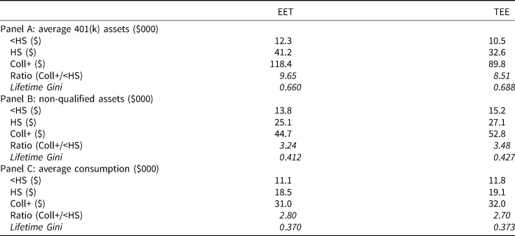
Notes: The first three rows of each panel report outcomes by educational group for the two tax regimes. The fourth row computes the ratio of Coll+ to <HS. Expected values are based on 200,000 simulated lifecycles allocated using population weights to the six-subgroups (male/female and three education groups) using optimal feedback controls from the life-cycle model. The Lifetime Gini coefficient is calculated year-by-year using 200,000 simulations for the entire population and averaged. For other parameters, see Figure 1.
Source: Authors' calculations.
The results generate some interesting conclusions. First, relative inequality measured as the ratio of average 401(k) assets of college graduates to high school dropouts falls by 12% in the TEE regime versus the EET regime. Second, relative inequality for cash on hand is 7% higher. Of course, as noted above, 401(k) assets cannot be directly compared across the two tax regimes, since in the EET world, these are subject to tax on withdrawal but not in the TEE regime. Moreover, the marginal tax rate for <HS individuals having only about $14,000 in their 401(k) accounts is far lower than for their Coll+ counterparts with over $210,000 in their 401(k) accounts. In consumption terms, then, the two tax regimes generate quite similar relative inequality metrics: the relative consumption inequality ratio under TEE is only 4% lower than in the EET case.
The last line of each panel in Table 2 reports average lifetime Gini coefficients under each tax regime. Rather strikingly, results indicate that the Gini measures are strikingly similar under the EET and the TEE regimes for lifetime consumption, assets in non-qualified accounts, and 401(k) assets, differing by only 1–4%. Therefore, we find few reasons that policymakers might favor either tax approach on egalitarian grounds.
3.2 Impacts on work hours and claiming ages
Table 3 depicts average work hours and Social Security claiming patterns under both the EET and TEE regimes. Panel A documents that Rothification induces people to work about one more hour per week until age 61, and three more hours per week during the Social Security claiming window (age 62–69). Panel B shows that Rothification pushes out retirement claiming by almost 1 year, compared to the EET base case.
Table 3. Social Security claiming ages and work hours under the EET versus TEE tax regime

Notes: Panel A reports average weekly work hours, while panel B shows average Social Security claiming ages for the two tax regimes. Expected values are based on 200,000 simulated lifecycles allocated using population weights to the six-subgroups (male/female and three education groups) using optimal feedback controls from the life-cycle model. For other parameters, see Figure 1.
Source: Authors' calculations.
The fact that the TEE regime's lower marginal tax rate on 401(k) payouts induces workers to delay Social Security claiming more than under the EET regime can be explained as follows: some workers with sufficient assets will wish to retire, but they also find it attractive to wait to claim Social Security so as to boost their benefits via the delayed claiming factor (6–8% increase per year of delayed claiming). Meanwhile, financing consumption during this no- (or low-) work phase requires them to work at least part-time and draw down their 401(k) assets. Under the EET regime, individuals must pay income tax on their pension withdrawals, so the appeal of receiving higher Social Security benefits by delaying claiming must be weighed against the disadvantage of paying high income taxes on withdrawals. If the tax burden on withdrawals is heavier than the advantage of receiving higher Social Security benefits, it is rational to claim earlier. This tradeoff also incorporates the fact that only a portion of Social Security benefits are included in taxable income (up to 50% may be tax-free). Accordingly, the net-of-tax gain from delaying Social Security claiming is relatively small in the EET scenario. Such complex tax considerations are irrelevant under the TEE regime, because pension withdrawals are not counted as part of taxable income. Therefore, given their financial resources to finance consumption until claiming, workers in the TEE scenario base their decisions to delay claiming only on the retirement credits received from deferring Social Security.
Work hours and Social Security claiming ages also differ by educational levels across the two tax regimes, as shown in Figure 2. Panel A shows the difference in claiming ages for workers with <HS, HS, and Coll+ education, while panel B depicts the corresponding changes in average hours worked during the claiming window. Interestingly, claiming patterns of the least-educated high school dropouts is relatively similar in both tax regimes, mainly because this group saves and accumulates few assets compared to the better-educated, so taxes are less relevant to them. Moreover, the changes in claiming ages for this subgroup are small. For example, high school dropouts claim 5 months later under the TEE regime, whereas the most educated group (Coll+) defers claiming Social Security benefits by over a year in the TEE versus EET setup. Differences in hours worked follow a similar pattern: the least educated work fewer than 2 hours per week more, whereas the most educated work more by about 4 hours a week. Accordingly, more educated and wealthier workers are predicted to work more and claim substantially later under Rothification, with a much smaller impact on the less-educated.

Figure 2. Differences by education in average work hours and claiming ages under the EET versus TEE tax regime. Panel A: Change in average Social Security claiming age. Panel B: Change in average work hours (ages 62–69).
Notes: This figure reports the average claiming age differences (panel A) and work hour differences (panel B) comparing the TEE versus the EET regime, for workers with three education levels. Results are derived from 200,000 simulated lifecycles allocated using population weights to each subgroup based on optimal feedback controls from the life-cycle model. The endogenous retirement age is between ages 62–70. For other parameters, see Figure 1.
Source: Authors' calculations.
3.3 Impacts on tax payments over the lifecycle
In terms of tax payments, there are two conceptual differences between EET and TEE taxation: timing and risk. Focusing first on timing, income tax payments come earlier with TEE, because contributions cannot be deducted from taxable income, and investment returns on accumulated retirement assets have no impact on tax payments. In contrast, under the EET system, tax payments are not due until later in life when withdrawals are made from the retirement savings account in retirement. Furthermore, under EET taxation, future uncertain investment income influences the amount of tax paid via deferred taxation. Tax payments are levied on distributions from qualified retirement accounts; these in turn depend on uncertain investment returns. Because tax-deferred retirement accounts are regularly invested and much of it in risky equity holdings, EET tax payments are subject to the return/risk profiles of the financial markets. This mechanism does not apply to TEE retirement accounts taxed up front.
Of course, tax payments under both regimes do vary with uncertainty in labor income and in both cases, uncertain investment returns affect tax payments for assets outside retirement accounts. To complete the picture, penalty taxes for early withdrawals and payroll taxes must also be considered. We depict the results under both regimes in Figure 3.

Figure 3. Average lifetime tax payments by age under the EET versus TEE tax regime. Panel A: Average tax payments by age. Panel B: Standard deviation of tax payments by age. Panel C: Present value of expected tax payments by age.
Notes: Panel A reports average individual annual tax payments (the sum of income taxes, payroll taxes, and taxes on early withdrawals) over the lifecycle in the EET versus TEE case. Panel B reports the annual standard deviation of tax payments. Panel C reports the expected present value of taxes paid by age group using a discount rate of 1%. Outcomes are based on 200,000 simulated lifecycles allocated using populations weights to each of the six subgroups (male/female and three education groups) using optimal feedback controls from the life-cycle model. For other parameters, see Figure 1.
Source: Authors' calculations.
Specifically, we plot average individual yearly tax payments (payroll taxes, income taxes, and penalty taxes for early withdrawals) based on the 200,000 simulated lifecycle under the EET and TEE regimes. As anticipated, expected tax payments (panel A) under EET are lower during the first 25 years of the work life, since 401(k) contributions can deducted from taxable income; by contrast, under the TEE regime, workers must pay taxes on own and employer matching contributions. Yet the situation changes around age 50, when tax payments rise in the EET regime, and the difference is particularly marked between ages 62–70. Thereafter, tax payments in both the EET and TEE scenarios are relatively low.
The explanation for this is that, in both tax regimes, workers begin curtailing their work hours after age 50 and finance some consumption with 401(k) withdrawals. From age 60 onward, 401(k) withdrawals are not subject to the 10% penalty tax, while withdrawals from EET accounts are included in taxable income. The latter results in higher tax payments, as opposed to the TEE world.
The difference in tax payments is particularly large between ages 62 and 70. For example, at age 65, the annual EET tax payment averages $8,000, or about twice as large as in the Roth regime. This is driven by individuals who have relatively large accumulations in their 401(k) plans and use these assets to reduce their work hours, delay claiming Social Security benefits, and spend retirement assets to cover consumption until claiming. From age 70 onward, their 401(k) assets are mostly spent, so people withdraw only small amounts from their retirement plans. Hence, retirees in the EET world pay only slightly more taxes than those in the TEE world.
Turning to panel B of Figure 3, we see the standard deviations of yearly tax payments under both tax scenarios. Here, the EET regime clearly has more volatility on tax payments resulting from uncertain investment returns over the lifecycle. From age 60, when households begin to withdraw from their 401(k) accounts, the volatility of the EET tax payments is significantly higher than that in the TEE regime. From age 70, after all workers are retired and receiving secure Social Security payments, the EET tax volatility is about twice as high as in the TEE case. The reason is that households still hold substantial equity in their 401(k)s later in life. This has a knock-on effect on potential withdrawals and thus, in the EET case, also on tax payments.
Panel C of Figure 3 reports numerical values of the expected present value of lifetime tax payments for the two tax regimes under consideration (as of age 25), assuming a real discount rate of 1% (the risk-free rate). A first observation is that average tax payments are higher (about $10,000 more) under the TEE system until workers reach age 49. Yet between ages 50 and 69, workers in the EET regime pay $16,000 (in present value) and retirees from age 70 on pay $5,000 more than in the TEE world. Over the complete lifecycle, the expected present value of lifetime taxes is 4% higher ($12,000) in the EET world. As a result, we conclude that tax payments are initially higher early in life under the TEE regime, but slightly lower in the long run. And as noted above, the overall higher EET tax payments are also accompanied by higher volatility.
A subsequent question would be how to use the initial expected higher tax revenues from Rothification. The possibilities are many, such as reducing the government budget deficit, cutting other taxes, or increasing government spending. Nevertheless, this lies outside the limits of our microeconomic single-generation lifecycle. We leave for future research an extension of our model to an overlapping generations setting, while retaining the realistic (and important) institutional framework.
3.4 Robustness checks
Models such as ours which project possible household economic patterns rely on several assumptions, making sensitivity analysis useful to evaluate the robustness of our findings. To this end, Table 4 reports results for financial assets inside and outside of qualified retirement accounts, as well as average lifetime consumption, using different assumptions regarding mortality, the time discount factor, employer matching contributions, and access to the stock market outside retirement accounts
Table 4. Sensitivity analysis by education under the EET versus TEE tax regime
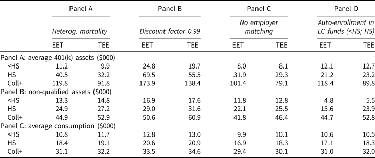
Notes: The first three rows of each panel report average lifetime assets in 401(k) accounts, cash on hand (non-retirement financial wealth), and consumption, respectively, by educational groups, for the two tax regimes. The first column labeled Heterogeneous mortality assumes higher (lower) mortality rates for workers with <HS (Coll+) compared to those with a HS education. Discount factor 0.99 refers to the case when the subjective discount factor is β = 0.99. No employer matching means no matching contributions are paid by the employer. Auto-enrollment in LC funds assumes 5% contribution of labor income is required in 401(k) plans (+ employer match) for the bottom two education groups; the assets are invested into life-cycle (LC) funds with age-dependent equity exposure (following the 100-age rule, see text) and only bond investments are held outside the retirement accounts. Expected values based on 200,000 simulated lifecycles allocated using population weights to the six-subgroups (male/female and three education groups) based on optimal feedback controls from the life-cycle model. For other parameters, see Table 3.
Source: Authors' calculations.
To start, we explore how results vary with alternative mortality assumptions by education group. Recent studies report widening mortality differentials by education, raising a question about whether the least-educated would benefit from moving from the status quo to a TEE tax regime. For instance, Kreuger et al. (Reference Kreuger, Tran, Hummer and Chang2015) reported that male high school dropouts averaged 23% excess mortality and females 32%, compared to high school graduates. By contrast, those with a college degree lived longer: men averaged a 6% lower mortality rate, and women 8%. Though only 10% of Americans have less than a high school degree and they comprise only 8% of the over-age 25 workforce (US DOL 2016), this group is more likely to be poor. Compared to the base case (see Table 2), average lifetime consumption, and financial assets inside and outside 401(k) plans decline slightly for the <HS group (panel A), while they rise for workers with a Coll+ education. This applies to both tax regimes EET and TEE. Therefore, the relative attractiveness of the two tax regimes barely changes, compared to the base case.
More substantial changes result if we reduce the time preference rate from 1 − β = 4%, as in the base case, to the level of the risk-free interest rate (1 − β = R f = 1%). As indicated in panel B, people in all three education groups and for both tax regimes build up much more financial wealth in retirement accounts compared to the base case. For example, high school dropouts save twice as much ($24,800 instead of $12,300) in their retirement accounts, compared to the base case with β = 0.96. Workers with a Coll+ education save about 50% more. Assets in non-qualified accounts also rise, but much less than retirement assets. The reason is that such assets mostly serve as precautionary savings to allow consumption smoothing against short-term shocks in labor or capital income. Average consumption also rises, mostly due to higher average working hours. Although the lower time preference rate does change consumption, labor supply, and financial wealth relative to the base case with a higher time preference rate, these changes have similar impacts under both the EET and TEE regimes. In other words, the relative attractiveness of the two tax regimes barely changes compared to the base case.
Next, we examine what happens when employers do not provide additional incentives to save via matching contributions (panel C), which allows us to examine the pure tax incentive effect to save for retirement. As expected, in this instance, fewer financial assets are accumulated in 401(k) plans relative to the base case. Yet clear differences can be observed across educational subgroups. High school dropouts save very little in 401(k) plans: the mean value of about $8,000 in 401(k) plans is lower than the $12,000 accumulated in non-qualified accounts. Interestingly, 401(k) assets for the TEE case are slightly higher ($8,100) for this education group than in the EET case ($8,000). The explanation lies in the relatively low incomes and thus low tax brackets of this lowest-earning group. In fact, many of these workers earn so little that they need not pay income taxes or may rely on government assistance. For them, retirement saving accounts offer few advantages, either tax-wise or through matching contributions, while they do impose liquidity restrictions. Consequently, these people save outside of retirement accounts, if at all. Only for a very few who earn relatively high incomes despite their low education (in the model, resulting from positive permanent income shocks) are the tax incentives sufficient to save for retirement in 401(k) accounts. In this case, TEE accounts are more attractive because they are associated with fewer liquidity constraints and are not taxed in retirement. This also explains the slight increase in consumption under the TEE versus the EET regime.
By contrast, workers with a Coll+ education face a different situation. The attractiveness of 401(k) plans is reduced due to no matching contributions, compared to the base case. Without employer matching contributions, mean 401(k) assets are lower by about 15% in the EET case (from $118,400 to $101,400). Yet 71% of total financial assets are still invested in retirement accounts; compared to the base case with 73%, for a very small reduction of 2 percentage points. In the TEE regime, the consequences are comparable, with about 12% less invested in 401(k) accounts, which continue to account (as in the base case) for 63% of total financial wealth. Thus, eliminating employer matching contributions does not dramatically change our conclusions about the relative impacts of EET versus TEE taxation.
As a last sensitivity analysis, we evaluate the impact of automatic enrollment in life-cycle funds as an alternative to assuming that workers can optimally make saving and portfolio allocation decisions. That is, to this point our model has assumed that households make rational economic decisions with the traditional expected utility framework, even though behavioral economists show that they sometimes do not, due to a host of reasons including financial illiteracy (Lusardi et al., Reference Lusardi, Mitchell and Michaud2017), inertia (Kim et al., Reference Kim, Maurer and Mitchell2016), loss or ambiguity aversion (Barberis and Huang, Reference Barberis and Huang2009), or ambiguity aversion (Dimmock et al., Reference Dimmock, Kouwenberg, Mitchell and Peijnenburg2016), among others. Unfortunately, there is no consensus in the literature regarding which and how behavioral aspects should be implemented in forward-looking normative models such as ours.
Accordingly, we focus here on two specific behavioral aspects which we can integrate into our life-cycle model in the form of numerically relatively easy-to-handle restrictions.Footnote 19 First, evidence documents that many US households do not participate in the stock market, especially with their non-retirement financial assets. To address this point, we now make the simplifying assumption that high school dropouts and graduates can only save in bonds outside their retirement accounts. Second, evidence shows also that some households have difficulty deciding how much to save in 401(k) plans and where to invest the contributions. To address this second point, we assume for the two low-educated groups that 5% of their incomes plus matching contributions are automatically enrolled into their 401(k) plan, which is then invested in a life-cycle fund with an age-dependent equity exposure according to the 100-age rule.Footnote 20 This restricts the decision space for these two population subgroups to work hours, claiming age, consumption, and 401(k) distributions. In this respect, this evaluation is not based on the usual ceteribus paribus approach (as in the other sensitivity analyses in Table 4), but rather it involves several model changes at once.
Results in panel D, Table 4, may be compared with those in Table 2. For high school dropouts, assets in the 401(k) setting are about the same in the EET regime, but about 20% higher in the TEE regime. Yet their cash on hand is much lower, averaging about one-third compared to the base case. The high school graduates hold almost 50% more 401(k) assets in the EET scenario and 29% more in the TEE regime, but their liquid asset holdings drop under both tax regimes. This is not due to low contribution rates, at these are relatively high at 5% of salary plus employer matches. Rather, it is the result of the life-cycle fund design: under the 100-age life investment rule, equity shares decline too quickly with age, compared to an optimal equity share. Overall, these changes affect results under both the EET and TEE tax scenarios similarly, and the relative attractiveness of the two tax regimes hardly differs from the base case.
4. Conclusions
This paper has evaluated whether adopting a different tax treatment for retirement plan contributions would materially change work hours, consumption, saving, asset allocations, and Social Security benefit claiming ages for individuals over their lifetimes. We also assess whether the lower-paid would behave differently from the higher-paid, in terms of changes in claiming, saving inside and outside retirement accounts, and non-pension saving.
We show that moving to a TEE system versus the current EET regime will have some interesting impacts on behavior, but modeling these outcomes is required due to the complex nonlinearities of tax and transfer systems in the USA. For example, the gap between high and low-wage workers' take-home pay is not diminished by income taxes under an EET system, whereas it is under a TEE program. Moreover, the Social Security replacement rate formula is concave, as it provides relatively higher benefits for low-wage workers than for the higher paid. Given these realities, the EET approach enhances the progressivity of overall old age income (pension account withdrawals plus Social Security benefits), whereas a TEE structure treats pension benefits more neutrally. Accordingly, it is theoretically impossible to predict how Rothification will alter household behavior without taking into account the complex institutional details confronting real-world consumers, along with the economic environment, capital and labor market risk, and uncertain lifetimes.
Our richly specified sophisticated structural model of lifetime behavior is calibrated to US federal/state income tax and Social Security/Medicare premium structures, along with realistic Social Security benefit rules including PIA and AIME formulas, early and delayed retirement adjustments under Social Security, and real-world rules characterizing tax-qualified DC accounts including the current caps on pre-tax contributions, employer matches, and penalties and taxes on early withdrawals. We find that taxing pension contributions instead of withdrawals leads to delayed retirement, somewhat lower lifetime tax payments, and relatively small reductions in consumption. Indeed, the two tax regimes generate quite similar relative inequality metrics: the relative consumption inequality ratio under TEE is only 4% higher than in the EET case. Moreover, results indicate that the Gini measures are also strikingly similar under the EET and the TEE regimes for lifetime consumption, cash on hand, and 401(k) assets, differing by only 1–4%. We therefore find few reasons for policymakers to favor either tax approach on egalitarian grounds.
We also investigate the impact on taxes paid over the complete lifecycle, and we document that the expected present value of lifetime taxes is 4% higher in the EET world. While tax payments are initially higher early in life under the TEE regime, they are slightly lower in the long run. Moreover, higher EET tax payments are also accompanied by higher volatility. Four different sensitivity analyses show that the relative attractiveness of the two tax regimes hardly differs from the base case.
These quantitative results regarding tax revenues should be interpreted with caution, since our microeconomic single-generation life-cycle model does not take into account potential macroeconomic effects that could arise with overlapping generations. Moreover, our model does not endogenize the impact of changes in the tax rules on the labor, financial, and goods markets. Nevertheless, since individual behaviors transfer to the macroeconomic level, our results indicate the direction of how Rothification of tax-qualified retirement accounts could affect the federal budget.
Supplementary material
The supplementary material for this article can be found at https://doi.org/10.1017/S1474747222000105.
Acknowledgments
The authors acknowledge research support for this work from the Michigan Retirement and Disability Research Center (MRDRC), the German Investment and Asset Management Association (BVI), and the Pension Research Council/Boettner Center at The Wharton School of the University of Pennsylvania. The authors also acknowledge the initiative High Performance Computing in Hessen for grating us computing time at the LOEWE-CSC and Lichtenberg Cluster. The authors thank Anna Maria Maurer for helpful comments. All findings and conclusions expressed are those of the authors and not the official views of the MRDRC, the Social Security Administration, or any of the other institutions with which the authors are affiliated. This research is part of the NBER Aging program and the Household Portfolio workshop. © 2022 Horneff, Maurer, and Mitchell.


 Open access