


1 Introduction
For algebraic vector bundles with an appropriate orientation, there are Euler classes and numbers enriched in bilinear forms. We will start over a field k and then discuss more general base schemes, obtaining integrality results. Let
 $\mathrm {GW}(k)$
denote the Grothendieck–Witt group of k, defined to be the group completion of the semi-ring of nondegenerate, symmetric, k-valued, bilinear forms (see, e.g., [Reference Lam53]). Let
$\mathrm {GW}(k)$
denote the Grothendieck–Witt group of k, defined to be the group completion of the semi-ring of nondegenerate, symmetric, k-valued, bilinear forms (see, e.g., [Reference Lam53]). Let
 $\langle a \rangle $
in
$\langle a \rangle $
in
 $\mathrm {GW}(k)$
denote the class of the rank
$\mathrm {GW}(k)$
denote the class of the rank
 $1$
bilinear form
$1$
bilinear form
 $(x,y) \mapsto axy$
for a in
$(x,y) \mapsto axy$
for a in
 $k^*$
.
$k^*$
.
For a smooth, proper k-scheme
 $f: X \to \operatorname {Spec} k $
of dimension n, coherent duality defines a trace map
$f: X \to \operatorname {Spec} k $
of dimension n, coherent duality defines a trace map
 $\eta _f: \mathrm {H}^n(X, \omega _{X/k}) \to k$
, which can be used to construct the following Euler number in
$\eta _f: \mathrm {H}^n(X, \omega _{X/k}) \to k$
, which can be used to construct the following Euler number in
 $\mathrm {GW}(k)$
. Let
$\mathrm {GW}(k)$
. Let
 $V \to X$
be a rank n vector bundle equipped with a relative orientation, meaning a line bundle
$V \to X$
be a rank n vector bundle equipped with a relative orientation, meaning a line bundle
 $\mathcal L$
on X and an isomorphism
$\mathcal L$
on X and an isomorphism
 $$ \begin{align*}\rho: \det V \otimes \omega_{X/k} \to \mathcal L^{\otimes 2}.\end{align*} $$
For
 $0 \leq i, j \leq n$
, let
$0 \leq i, j \leq n$
, let
 $\beta _{i,j}$
denote the perfect pairing
$\beta _{i,j}$
denote the perfect pairing
 $$ \begin{align} \beta_{i,j}: \mathrm{H}^i\left(X, \wedge^j V^* \otimes \mathcal L\right) \otimes \mathrm{H}^{n-i}\left(X, \wedge^{n-j} V^* \otimes \mathcal L\right)\to k\end{align} $$
given by the composition
 $$ \begin{align*}\mathrm{H}^i\left(X, \wedge^j V^* \otimes \mathcal L\right) \otimes \mathrm{H}^{n-i}\left(X, \wedge^{n-j} V^* \otimes \mathcal L\right) \stackrel{\cup}{\to} \mathrm{H}^n\left(X, \wedge^n V^* \otimes \mathcal L^{\otimes 2}\right) \stackrel{\rho}{\to} \mathrm{H}^n(X, \omega_{X/k}) \stackrel{\eta_f}{\to} k.\end{align*} $$
For
 $i = n-i$
and
$i = n-i$
and
 $j=n-j$
, note that
$j=n-j$
, note that
 $\beta _{i,j}$
is a bilinear form on
$\beta _{i,j}$
is a bilinear form on
 $ \mathrm {H}^i\left (X, \wedge ^j V^* \otimes \mathcal L\right )$
. Otherwise,
$ \mathrm {H}^i\left (X, \wedge ^j V^* \otimes \mathcal L\right )$
. Otherwise,
 $\beta _{i,j} \oplus \beta _{n-i,n-j}$
determines the bilinear form on
$\beta _{i,j} \oplus \beta _{n-i,n-j}$
determines the bilinear form on
 $\mathrm {H}^i\left (X, \wedge ^j V^* \otimes \mathcal L\right ) \oplus \mathrm {H}^{n-i}\left (X, \wedge ^{n-j} V^* \otimes \mathcal L\right )$
. The alternating sum
$\mathrm {H}^i\left (X, \wedge ^j V^* \otimes \mathcal L\right ) \oplus \mathrm {H}^{n-i}\left (X, \wedge ^{n-j} V^* \otimes \mathcal L\right )$
. The alternating sum
 $$ \begin{align*}n^{\mathrm{GS}}(V) : = \sum_{0 \leq i, j \leq n} (-1)^{i+j}\beta_{i,j}\end{align*} $$
thus determines an element of
 $\mathrm {GW}(k)$
, which we will call the Grothendieck–Serre duality or coherent duality Euler number. Note that
$\mathrm {GW}(k)$
, which we will call the Grothendieck–Serre duality or coherent duality Euler number. Note that
 $\beta _{i,j} \oplus \beta _{n-i,n-j}$
in
$\beta _{i,j} \oplus \beta _{n-i,n-j}$
in
 $\mathrm {GW}(k)$
is an integer multiple of h, where h denotes the hyperbolic form
$\mathrm {GW}(k)$
is an integer multiple of h, where h denotes the hyperbolic form
 $h = \langle 1 \rangle + \langle -1 \rangle $
, with Gram matrix
$h = \langle 1 \rangle + \langle -1 \rangle $
, with Gram matrix
 $$ \begin{align*}h= \left[ {\begin{array}{cc} 0 & 1 \\ 1 & 0 \\ \end{array}}\right].\end{align*} $$
This notion of the Euler number was suggested by M. J. Hopkins, J.-P. Serre, and A. Raksit, and developed by M. Levine and Raksit for the tangent bundle in [Reference Levine and Raksit56].
For a relatively oriented vector bundle V equipped with a section
 $\sigma $
with only isolated zeros, an Euler number
$\sigma $
with only isolated zeros, an Euler number
 $n^{\mathrm {PH}}(V, \sigma )$
was defined in [Reference Kass and Wickelgren49, Section 4] as a sum of local indices:
$n^{\mathrm {PH}}(V, \sigma )$
was defined in [Reference Kass and Wickelgren49, Section 4] as a sum of local indices:
 $$ \begin{align*}n^{\mathrm{PH}}(V, \sigma) = \sum_{x : \sigma(x) = 0} \mathrm{ind}^{\mathrm{PH}}_x \sigma .\end{align*} $$
The index
 $\mathrm {ind}^{\mathrm {PH}}_x \sigma $
can be computed explicitly with a formula of Scheja and Storch [Reference Scheja and Storch67] or of Eisenbud and Levine/Khimshiashvili [Reference Eisenbud and Levine29] (see §§2.4 and 2.3) and is also a local degree [Reference Kass and Wickelgren48] (this is discussed further in §7). For example, when x is a simple zero of
$\mathrm {ind}^{\mathrm {PH}}_x \sigma $
can be computed explicitly with a formula of Scheja and Storch [Reference Scheja and Storch67] or of Eisenbud and Levine/Khimshiashvili [Reference Eisenbud and Levine29] (see §§2.4 and 2.3) and is also a local degree [Reference Kass and Wickelgren48] (this is discussed further in §7). For example, when x is a simple zero of
 $\sigma $
with
$\sigma $
with
 $k(x)=k$
, the index is given by a well-defined Jacobian
$k(x)=k$
, the index is given by a well-defined Jacobian
 $\mathrm {Jac}\sigma $
of
$\mathrm {Jac}\sigma $
of
 $\sigma $
,
$\sigma $
,
 $$ \begin{align*}\mathrm{ind}^{\mathrm{PH}}_x \sigma= \langle \mathrm{Jac}\sigma(x) \rangle,\end{align*} $$
illustrating the relation with the Poincaré–Hopf formula for topological vector bundles. (For the definition of the Jacobian, see the beginning of §6.2.) In [Reference Kass and Wickelgren49, Section 4, Corollary 36], it was shown that
 $n^{\mathrm {PH}}(V, \sigma ) = n^{\mathrm {PH}}(V, \sigma ')$
when
$n^{\mathrm {PH}}(V, \sigma ) = n^{\mathrm {PH}}(V, \sigma ')$
when
 $\sigma $
and
$\sigma $
and
 $\sigma '$
are in a family over
$\sigma '$
are in a family over
 $\mathbb A^1_L$
of sections with only isolated zeros, where L is a field extension with
$\mathbb A^1_L$
of sections with only isolated zeros, where L is a field extension with
 $[L:k]$
odd. We strengthen this result by equating
$[L:k]$
odd. We strengthen this result by equating
 $n^{\mathrm {PH}}(V, \sigma )$
and
$n^{\mathrm {PH}}(V, \sigma )$
and
 $n^{\mathrm {GS}}(V)$
; this is the main result of §2.
$n^{\mathrm {GS}}(V)$
; this is the main result of §2.
Theorem 1.1 see §2.4
Let k be a field and
 $V \to X$
be a relatively oriented, rank n vector bundle on a smooth, proper k-scheme of dimension n. Suppose V has a section
$V \to X$
be a relatively oriented, rank n vector bundle on a smooth, proper k-scheme of dimension n. Suppose V has a section
 $\sigma $
with only isolated zeros. Then
$\sigma $
with only isolated zeros. Then
 $$ \begin{align*}n^{\mathrm{PH}}(V, \sigma) = n^{\mathrm{GS}}(V).\end{align*} $$
In particular,
 $n^{\mathrm {PH}}(V, \sigma )$
is independent of the choice of
$n^{\mathrm {PH}}(V, \sigma )$
is independent of the choice of
 $\sigma $
.
$\sigma $
.
Remark 1.2 Theorem 1.1 strengthens [Reference Bethea, Kass and Wickelgren15], removing its hypothesis (2) entirely. It also simplifies the proofs of [Reference Kass and Wickelgren49, Theorem 1] and [Reference Srinivasan and Wickelgren72, Theorems 1 and 2]: it is no longer necessary to show that the sections of certain vector bundles with nonisolated isolated zeros are of codimension
 $2$
, as in [Reference Kass and Wickelgren49, Lemmas 54, 56, and 57] and in [Reference Srinivasan and Wickelgren72, Lemma 1], because
$2$
, as in [Reference Kass and Wickelgren49, Lemmas 54, 56, and 57] and in [Reference Srinivasan and Wickelgren72, Lemma 1], because
 $n^{\mathrm {PH}}(V, \sigma )$
is independent of
$n^{\mathrm {PH}}(V, \sigma )$
is independent of
 $\sigma $
.
$\sigma $
.
1.1 Sketch proof and generalizations
The proof of Theorem 1.1 proceeds in three steps:
-
(0) For a section
 $\sigma $
of V, we define an Euler number relative to the section using coherent duality and denote it by
$n^{\mathrm {GS}}(V, \sigma , \rho )$
. If
$\sigma = 0$
, we recover the absolute Euler number
$n^{\mathrm {GS}}(V, \rho )$
, essentially by construction.
$\sigma $
of V, we define an Euler number relative to the section using coherent duality and denote it by
$n^{\mathrm {GS}}(V, \sigma , \rho )$
. If
$\sigma = 0$
, we recover the absolute Euler number
$n^{\mathrm {GS}}(V, \rho )$
, essentially by construction. -
(1) For two sections
$\sigma _1, \sigma _2$
, we show that
$n^{\mathrm {GS}}(V, \sigma _1, \rho ) = n^{\mathrm {GS}}(V, \sigma _2, \rho )$
. To prove this, one can use homotopy invariance of Hermitian K-theory or show that
$n^{\mathrm {GS}}(V, \sigma _1, \rho ) = n^{\mathrm {GS}}(V, \rho )$
by showing an instance of the principle that alternating sums, like Euler characteristics, are unchanged by passing to the homology of a complex. -
(2) If a section
$\sigma $
has isolated zeros, then
$n^{\mathrm {GS}}(V, \sigma , \rho )$
can be expressed as a sum of local indices
$\mathrm {ind}_{Z/S}(\sigma )$
, where Z is (a clopen component of) the zero scheme of
$\sigma $
. -
(3) For Z a local complete intersection in affine space–that is, in the presence of coordinates – we compute the local degree explicitly and identify it with the Scheja–Storch form [Reference Ananyevskiy2, Reference Scheja and Storch67].


Taken together, these steps show that
 $n^{\mathrm {GS}}(V, \rho )$
is a sum of local contributions given by Scheja–Storch forms, which is essentially the definition of
$n^{\mathrm {GS}}(V, \rho )$
is a sum of local contributions given by Scheja–Storch forms, which is essentially the definition of
 $n^{\mathrm {PH}}(V, \rho )$
.
$n^{\mathrm {PH}}(V, \rho )$
.
These arguments can be generalized considerably, replacing the Grothendieck–Witt group
 $\mathrm {GW}$
by a more general cohomology theory E. We need E to admit transfers along proper lci morphisms of schemes, and an
$\mathrm {GW}$
by a more general cohomology theory E. We need E to admit transfers along proper lci morphisms of schemes, and an
 $\mathrm {SL}^c$
-orientation (see §3 for more details). Then for step (0) one can define an Euler class
$\mathrm {SL}^c$
-orientation (see §3 for more details). Then for step (0) one can define an Euler class
 $e(V, \sigma , \rho )$
as
$e(V, \sigma , \rho )$
as
 $z^*\sigma _*(1)$
, where z is the zero section. Step (2) is essentially formal; the main content is in steps (1) and (3). Step (1) becomes formal if we assume that E is
$z^*\sigma _*(1)$
, where z is the zero section. Step (2) is essentially formal; the main content is in steps (1) and (3). Step (1) becomes formal if we assume that E is
 $\mathbb A^1$
-invariant. In particular, steps (0)–(2) can be performed for
$\mathbb A^1$
-invariant. In particular, steps (0)–(2) can be performed for
 $\mathrm {SL}$
-oriented cohomology theories represented by motivic spectra; this is explained in §§3, 4, and 5.
$\mathrm {SL}$
-oriented cohomology theories represented by motivic spectra; this is explained in §§3, 4, and 5.
It remains to find a replacement for step (3). We offer two possibilities: in §7 we show that, again in the presence of coordinates, the local indices can be identified with appropriate
 $\mathbb A^1$
-degrees. On the other hand, in §8 we show that for
$\mathbb A^1$
-degrees. On the other hand, in §8 we show that for
 $E = \mathrm {KO}$
the motivic spectrum corresponding to Hermitian K-theory, the local indices are again given by Scheja–Storch forms. This implies the following:
$E = \mathrm {KO}$
the motivic spectrum corresponding to Hermitian K-theory, the local indices are again given by Scheja–Storch forms. This implies the following:
Corollary 1.3 see Corollary 8.2 and Definition 3.10
Let
 $S=Spec(k)$
, where k is a field of characteristic
$S=Spec(k)$
, where k is a field of characteristic
 $\ne 2$
.Footnote 1 Let
$\ne 2$
.Footnote 1 Let
 $\pi : X \to k$
be smooth and
$\pi : X \to k$
be smooth and
 $V/X$
a relatively oriented vector bundle with a nondegenerate section
$V/X$
a relatively oriented vector bundle with a nondegenerate section
 $\sigma $
. Write
$\sigma $
. Write
 $\varpi : Z=Z(\sigma ) \to k$
for the vanishing scheme (which need not be smooth). Then
$\varpi : Z=Z(\sigma ) \to k$
for the vanishing scheme (which need not be smooth). Then
 $$\begin{align*}n^{\mathrm{PH}}(V, \sigma) = \varpi_*(1) \in \mathrm{KO}^0(k) = \mathrm{GW}(k). \end{align*}$$
Here we have used the lci push-forward
 $$\begin{align*}\varpi_*: \mathrm{KO}^0(Z) \stackrel{\rho}{\simeq} \mathrm{KO}^{L_\varpi}(Z) \to \mathrm{KO}^0(k) \end{align*}$$
of Déglise, Jin, and Khan [Reference Déglise, Jin and Khan26]. If, moreover, X is proper, then
 $\varpi _*(1)$
also coincides with
$\varpi _*(1)$
also coincides with
 $\pi _*z^*z_*(1)$
, where
$\pi _*z^*z_*(1)$
, where
 $z: X \to V$
is the zero section (see Corollaries 5.18 and 5.21 and Proposition 5.19). This provides an alternative proof that
$z: X \to V$
is the zero section (see Corollaries 5.18 and 5.21 and Proposition 5.19). This provides an alternative proof that
 $n^{\mathrm {PH}}(V,\sigma )$
is independent of the choice of
$n^{\mathrm {PH}}(V,\sigma )$
is independent of the choice of
 $\sigma $
(under our assumption on k).
$\sigma $
(under our assumption on k).
Another important example is when E is taken to be the motivic cohomology theory representing Chow–Witt groups. This recovers the Barge–Morel Euler class
 $e^{\mathrm {BM}}(V)$
in
$e^{\mathrm {BM}}(V)$
in
 $\widetilde {\mathrm {CH}}^r(X, \det V^*)$
[Reference Barge and Morel12], which is defined for a base field of characteristic not
$\widetilde {\mathrm {CH}}^r(X, \det V^*)$
[Reference Barge and Morel12], which is defined for a base field of characteristic not
 $2$
. Suppose that
$2$
. Suppose that
 $\rho $
is a relative orientation of V and
$\rho $
is a relative orientation of V and
 $\pi : X \to \operatorname {Spec} k$
is the structure map.
$\pi : X \to \operatorname {Spec} k$
is the structure map.
Corollary 1.4. Let k be a field of characteristic
 $\ne 2$
. Then
$\ne 2$
. Then
 $\pi _* e^{\mathrm {BM}}(V, \rho ) = n^{\mathrm {GS}}(V, \rho )$
in
$\pi _* e^{\mathrm {BM}}(V, \rho ) = n^{\mathrm {GS}}(V, \rho )$
in
 $\mathrm {GW}(k)$
.
$\mathrm {GW}(k)$
.
Proof. We have
 $e^{\mathrm {BM}}(V, \rho ) = e\left (V, \rho , H\tilde {\mathbb {Z}}\right )$
; indeed, by Proposition 5.19,
$e^{\mathrm {BM}}(V, \rho ) = e\left (V, \rho , H\tilde {\mathbb {Z}}\right )$
; indeed, by Proposition 5.19,
 $e\left (V, \rho , H\tilde {\mathbb {Z}}\right )$
can be computed in terms of push-forward along the zero section of V, and exactly the same is true for
$e\left (V, \rho , H\tilde {\mathbb {Z}}\right )$
can be computed in terms of push-forward along the zero section of V, and exactly the same is true for
 $e^{\mathrm {BM}}$
by definition [Reference Barge and Morel12, §2.1]. We also have
$e^{\mathrm {BM}}$
by definition [Reference Barge and Morel12, §2.1]. We also have
 $n^{\mathrm {GS}}(V,\rho ) = n(V, \rho , \mathrm {KO})$
; indeed, the right-hand side is represented by the natural symmetric bilinear form on the cohomology of the Koszul complex by Example 8.1, and this is essentially the definition of
$n^{\mathrm {GS}}(V,\rho ) = n(V, \rho , \mathrm {KO})$
; indeed, the right-hand side is represented by the natural symmetric bilinear form on the cohomology of the Koszul complex by Example 8.1, and this is essentially the definition of
 $n^{\mathrm {GS}}(V,\rho )$
.
$n^{\mathrm {GS}}(V,\rho )$
.
It thus suffices to prove that
 $n\left (V, \rho , H\tilde {\mathbb {Z}}\right ) = n(V, \rho , \mathrm {KO}) \in \mathrm {GW}(k)$
. Consider the span of ring spectra
$n\left (V, \rho , H\tilde {\mathbb {Z}}\right ) = n(V, \rho , \mathrm {KO}) \in \mathrm {GW}(k)$
. Consider the span of ring spectra
 $H\tilde {\mathbb {Z}} \leftarrow \tilde f_0 \mathrm {KO} \to \mathrm {KO}$
as in the proof of Proposition 5.4. It induces an isomorphism on
$H\tilde {\mathbb {Z}} \leftarrow \tilde f_0 \mathrm {KO} \to \mathrm {KO}$
as in the proof of Proposition 5.4. It induces an isomorphism on
 $\pi _0(\mathord -)(k)$
, namely with
$\pi _0(\mathord -)(k)$
, namely with
 $\mathrm {GW}(k)$
in all cases. The desired equality follows from the naturality of the Euler numbers.
$\mathrm {GW}(k)$
in all cases. The desired equality follows from the naturality of the Euler numbers.
(An alternative argument proceeds as follows: It suffices to prove that
 $\pi _* e^{\mathrm {BM}}(V,\rho )$
and
$\pi _* e^{\mathrm {BM}}(V,\rho )$
and
 $n^{\mathrm {GS}}(V, \rho )$
have the same image in
$n^{\mathrm {GS}}(V, \rho )$
have the same image in
 $\mathrm {W}(k)$
and
$\mathrm {W}(k)$
and
 $\mathbb {Z}$
. The image of
$\mathbb {Z}$
. The image of
 $n^{\mathrm {GS}}(V, \rho )$
in
$n^{\mathrm {GS}}(V, \rho )$
in
 $\mathrm {W}(k$
) is given by
$\mathrm {W}(k$
) is given by
 $n(V, \rho , \mathrm {KW})$
; for this we need only show that
$n(V, \rho , \mathrm {KW})$
; for this we need only show that
 $e(V,\rho ,\mathrm {KW})$
is represented by the Koszul complex, which is Example 5.20. It will thus be enough to show that
$e(V,\rho ,\mathrm {KW})$
is represented by the Koszul complex, which is Example 5.20. It will thus be enough to show that
 $n(V, \rho , H\mathbb {Z}) = n(V, \rho , \mathrm {KGL})$
and
$n(V, \rho , H\mathbb {Z}) = n(V, \rho , \mathrm {KGL})$
and
 $n\left (V, \rho , \underline {W}\left [\eta ^{\pm }\right ]\right ) = n(V, \rho , \mathrm {KW})$
; this follows as before by considering the spans
$n\left (V, \rho , \underline {W}\left [\eta ^{\pm }\right ]\right ) = n(V, \rho , \mathrm {KW})$
; this follows as before by considering the spans
 $H\mathbb {Z} \leftarrow \mathrm {kgl} \to \mathrm {KGL}$
and
$H\mathbb {Z} \leftarrow \mathrm {kgl} \to \mathrm {KGL}$
and
 $\underline {W}\left [\eta ^{\pm }\right ] \leftarrow \mathrm {KW}_{\ge 0} \to \mathrm {KW}$
.)Footnote 2
$\underline {W}\left [\eta ^{\pm }\right ] \leftarrow \mathrm {KW}_{\ge 0} \to \mathrm {KW}$
.)Footnote 2
The left-hand side is the Euler class studied by M. Levine in [Reference Levine55]. We do not compare these Euler classes with the obstruction-theoretic Euler class of [Reference Morel61, Chapter 8]. Asok and Fasel show that the latter agrees with
 $\pi _* e^{\mathrm {BM}}(V, \rho )$
up to a unit in
$\pi _* e^{\mathrm {BM}}(V, \rho )$
up to a unit in
 $\mathrm {GW}(k)$
[Reference Asok and Fasel3].
$\mathrm {GW}(k)$
[Reference Asok and Fasel3].
1.2 Applications
It is straightforward to see that Euler numbers for cohomology theories are stable under base change (see Corollary 5.3). This implies that in considering vector bundles on varieties which are already defined over, for example,
 $\operatorname {Spec}(\mathbb {Z}[1/2])$
, the possible Euler numbers are constrained to live in
$\operatorname {Spec}(\mathbb {Z}[1/2])$
, the possible Euler numbers are constrained to live in
 $\mathrm {GW}(\mathbb {Z}[1/2]) = \mathbb {Z}[\langle -1 \rangle , \langle 2 \rangle ] \subset \mathrm {GW}(\mathbb {Q})$
. Using novel results on Hermitian K-theory [Reference Calmès, Dotto, Harpaz, Hebestreit, Land, Moi, Nardin, Nikolaus and Steimle18] allows one to use the base scheme
$\mathrm {GW}(\mathbb {Z}[1/2]) = \mathbb {Z}[\langle -1 \rangle , \langle 2 \rangle ] \subset \mathrm {GW}(\mathbb {Q})$
. Using novel results on Hermitian K-theory [Reference Calmès, Dotto, Harpaz, Hebestreit, Land, Moi, Nardin, Nikolaus and Steimle18] allows one to use the base scheme
 $\operatorname {Spec} \mathbb {Z}$
as well. Proposition 5.4 contains both of these cases, and the
$\operatorname {Spec} \mathbb {Z}$
as well. Proposition 5.4 contains both of these cases, and the
 $\mathbb {Z}[1/2]$
case is independent of [Reference Calmès, Dotto, Harpaz, Hebestreit, Land, Moi, Nardin, Nikolaus and Steimle18]. It follows that for relatively oriented bundles over
$\mathbb {Z}[1/2]$
case is independent of [Reference Calmès, Dotto, Harpaz, Hebestreit, Land, Moi, Nardin, Nikolaus and Steimle18]. It follows that for relatively oriented bundles over
 $\mathbb {Z}$
the Euler numbers can be read off from topological computations (Proposition 5.9). Over
$\mathbb {Z}$
the Euler numbers can be read off from topological computations (Proposition 5.9). Over
 $\mathbb {Z}[1/2]$
the topological Euler numbers of the associated real and complex vector bundles, together with one further algebraic computation over some field in which
$\mathbb {Z}[1/2]$
the topological Euler numbers of the associated real and complex vector bundles, together with one further algebraic computation over some field in which
 $2$
is not a square, determine the Euler number (and this is again independent of [Reference Calmès, Dotto, Harpaz, Hebestreit, Land, Moi, Nardin, Nikolaus and Steimle18]); see Theorem 5.11.
$2$
is not a square, determine the Euler number (and this is again independent of [Reference Calmès, Dotto, Harpaz, Hebestreit, Land, Moi, Nardin, Nikolaus and Steimle18]); see Theorem 5.11.
We use this to compute a weighted count of d-dimensional hyperplanes in a general complete intersection
 $$ \begin{align*}\left\{f_1 = \cdots = f_j \right\} \hookrightarrow \mathbb P^n_k\end{align*} $$
over a field k. This count depends only on the degrees of the polynomials
 $f_i$
and not on the
$f_i$
and not on the
 $f_i$
themselves: it is determined by associated real and complex counts, for any d and degrees such that the expected variety of d-planes is
$f_i$
themselves: it is determined by associated real and complex counts, for any d and degrees such that the expected variety of d-planes is
 $0$
-dimensional and the associated real count is defined. This is Corollary 6.9. For example, combining with results of Finashin and Kharlamov over
$0$
-dimensional and the associated real count is defined. This is Corollary 6.9. For example, combining with results of Finashin and Kharlamov over
 $\mathbb {R}$
[Reference Finashin and Kharlamov34], we have that
$\mathbb {R}$
[Reference Finashin and Kharlamov34], we have that
 $160,839 \langle 1 \rangle + 160,650 \langle -1 \rangle $
and
$160,839 \langle 1 \rangle + 160,650 \langle -1 \rangle $
and
 $$ \begin{align*} &32,063,862,647,475,902,965,720,976,420,325 \langle 1 \rangle\\ &\quad {}+ 32,063,862,647,475,902,965,683,320,692,800 \langle -1 \rangle\end{align*} $$
are arithmetic counts of the
 $3$
-planes in a
$3$
-planes in a
 $7$
-dimensional cubic hypersurface and in a
$7$
-dimensional cubic hypersurface and in a
 $16$
-dimensional degree
$16$
-dimensional degree
 $5$
hypersurface, respectively (see Example 6.13). This builds on results of Finashin and Kharlamov [Reference Finashin and Kharlamov34], J. L. Kass and the second author of the present paper [Reference Kass and Wickelgren49], M. Levine [Reference Levine54], S. McKean [Reference McKean58], Okonek and Teleman [Reference Okonek and Teleman62], S. Pauli [Reference Pauli66], J. Solomon [Reference Solomon70], P. Srinivasan and the second author [Reference Srinivasan and Wickelgren72], and M. Wendt [Reference Wendt74].
$5$
hypersurface, respectively (see Example 6.13). This builds on results of Finashin and Kharlamov [Reference Finashin and Kharlamov34], J. L. Kass and the second author of the present paper [Reference Kass and Wickelgren49], M. Levine [Reference Levine54], S. McKean [Reference McKean58], Okonek and Teleman [Reference Okonek and Teleman62], S. Pauli [Reference Pauli66], J. Solomon [Reference Solomon70], P. Srinivasan and the second author [Reference Srinivasan and Wickelgren72], and M. Wendt [Reference Wendt74].
1.3 Notation and conventions
1.3.1 Grothendieck duality
We believe that if
 $f: X \to Y$
is a morphism of schemes which is locally of finite presentation, then there is a well-behaved adjunction
$f: X \to Y$
is a morphism of schemes which is locally of finite presentation, then there is a well-behaved adjunction
 $$\begin{align*}f_!: D_{\mathrm{qcoh}}(X) \leftrightarrows D_{\mathrm{qcoh}}(Y): f^! \end{align*}$$
between the associated derived (
 $\infty $
-)categories of unbounded complexes of
$\infty $
-)categories of unbounded complexes of
 $\mathcal O_X$
-modules with quasi-coherent homology sheaves. Unfortunately, we are not aware of any references in this generality. Instead, whenever mentioning a functor
$\mathcal O_X$
-modules with quasi-coherent homology sheaves. Unfortunately, we are not aware of any references in this generality. Instead, whenever mentioning a functor
 $f^!$
, we implicitly assume that X and Y are separated and of finite type over some Noetherian scheme S. In this situation, the functor
$f^!$
, we implicitly assume that X and Y are separated and of finite type over some Noetherian scheme S. In this situation, the functor
 $f^!$
is constructed for homologically bounded-above complexes in [73, Tag 0A9Y] (see also [ Reference Conrad24, Reference Hartshorne40]), and this is all we will use.
$f^!$
is constructed for homologically bounded-above complexes in [73, Tag 0A9Y] (see also [ Reference Conrad24, Reference Hartshorne40]), and this is all we will use.
1.3.2 Vector bundles
We identify locally free sheaves and vector bundles covariantly, via the assignment
 $$\begin{align*}\mathcal E \leftrightarrow \operatorname{Spec}(\operatorname{Sym}(\mathcal E^*)). \end{align*}$$
While it can be convenient to (not) pass to duals here (as in, e.g., [Reference Déglise, Jin and Khan26]), we do not do this, because it confuses the first author terribly.
1.3.3 Regular sequences and immersions
Following, for example, [Reference Berthelot, Grothendieck et, Illusie, Jouanolou, Jussila, Kleiman, Raynaud et and Serre14], by a regular immersion of schemes we mean what is called a Koszul-regular immersion in [73, Tag 0638]–that is, a morphism which is locally a closed immersion cut out by a Koszul-regular sequence. Moreover, by a regular sequence we will always mean a Koszu-regular sequence [73, Tag 062D], and we reserve the term strongly regular sequence for the usual notion. A strongly regular sequence is regular [73, Tag 062F], whence a strongly regular immersion is regular. In locally Noetherian situations, regular immersions are strongly regular [73, Tags 063L].
1.3.4 Cotangent complexes
For a morphism
 $f: X \to Y$
, we write
$f: X \to Y$
, we write
 $L_f$
for the cotangent complex. Recall that if f is smooth, then
$L_f$
for the cotangent complex. Recall that if f is smooth, then
 $L_f \simeq \Omega _f$
, whereas if f is a regular immersion, then
$L_f \simeq \Omega _f$
, whereas if f is a regular immersion, then
 $L_f \simeq C_f[1]$
, where
$L_f \simeq C_f[1]$
, where
 $C_f$
denotes the conormal bundle.
$C_f$
denotes the conormal bundle.
1.3.5 Graded determinants
We write
 $\widetilde \det : K(X) \to \mathrm {Pic}(D(X))$
for the determinant morphism from Thomason–Trobaugh K-theory to the groupoid of graded line bundles. If C is a perfect complex, then we write
$\widetilde \det : K(X) \to \mathrm {Pic}(D(X))$
for the determinant morphism from Thomason–Trobaugh K-theory to the groupoid of graded line bundles. If C is a perfect complex, then we write
 $\widetilde \det C$
for the determinant of the associated K-theory point. We write
$\widetilde \det C$
for the determinant of the associated K-theory point. We write
 $\det C \in \mathrm {Pic}(X)$
for the ungraded determinant.
$\det C \in \mathrm {Pic}(X)$
for the ungraded determinant.
Given an lci morphism f, we set
 $\omega _f = \det L_f$
and
$\omega _f = \det L_f$
and
 $\widetilde \omega _f = \widetilde \det L_f$
.
$\widetilde \omega _f = \widetilde \det L_f$
.
We systematically use graded determinants throughout the article; for example, we have the following compact definition of a relative orientation:
Definition 1.5. Let
 $\pi : X \to S$
be an lci morphism and V a vector bundle on X. By a relative orientation of
$\pi : X \to S$
be an lci morphism and V a vector bundle on X. By a relative orientation of
 $V/X/S$
we mean a choice of line bundle
$V/X/S$
we mean a choice of line bundle
 $\mathcal L$
on X and an isomorphism
$\mathcal L$
on X and an isomorphism
 $$\begin{align*}\rho: \underline{\operatorname{Hom}}\left(\widetilde\det V^*, \widetilde \omega_{X/S}\right) \xrightarrow{\simeq} \mathcal L^{\otimes 2}. \end{align*}$$
Note that if
 $\pi $
is smooth, this just means that the locally constant functions
$\pi $
is smooth, this just means that the locally constant functions
 $x \mapsto \operatorname {rank}(V_x)$
and
$x \mapsto \operatorname {rank}(V_x)$
and
 $x \mapsto \dim \pi ^{-1}(\pi (x))$
on X agree, and that we are given an isomorphism
$x \mapsto \dim \pi ^{-1}(\pi (x))$
on X agree, and that we are given an isomorphism
 $\mathcal L^{\otimes 2} \simeq \omega _{X/S} \otimes \det V$
. Hence we recover the definition from [Reference Kass and Wickelgren49, Definition 17].
$\mathcal L^{\otimes 2} \simeq \omega _{X/S} \otimes \det V$
. Hence we recover the definition from [Reference Kass and Wickelgren49, Definition 17].
2 Equality of coherent duality and Poincaré–Hopf Euler numbers
We prove Theorem 1.1 in this section.
2.1 Coherent-duality Euler Number
Let
 $f:X \to \operatorname {Spec} k$
be a smooth, proper k-scheme of dimension n, and let V be a rank n vector bundle, relatively oriented by the line bundle
$f:X \to \operatorname {Spec} k$
be a smooth, proper k-scheme of dimension n, and let V be a rank n vector bundle, relatively oriented by the line bundle
 $\mathcal L$
on X and the isomorphism
$\mathcal L$
on X and the isomorphism
 $\rho : \det V \otimes \omega _{X/k} \to \mathcal L^{\otimes 2}$
. Let
$\rho : \det V \otimes \omega _{X/k} \to \mathcal L^{\otimes 2}$
. Let
 $\sigma : X \to V$
be a section, and let
$\sigma : X \to V$
be a section, and let
 $K(\sigma )^\bullet $
denote the Koszul complex
$K(\sigma )^\bullet $
denote the Koszul complex
 $$\begin{align*}0 \to \wedge^n V^* \to \wedge^{n-1} V^* \to \cdots \to V^* \to \mathcal{O} \to 0, \end{align*}$$
with
 $\mathcal {O}$
in degree
$\mathcal {O}$
in degree
 $0$
and differential of degree
$0$
and differential of degree
 $+1$
given by
$+1$
given by
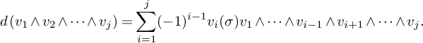 $$ \begin{align*}d\left(v_1 \wedge v_2 \wedge \cdots \wedge v_j\right) = \sum_{i=1}^j (-1)^{i-1} v_i(\sigma) v_1 \wedge \cdots \wedge v_{i-1} \wedge v_{i+1} \wedge \cdots \wedge v_j.\end{align*} $$
This choice of
 $K(\sigma )^{\bullet }$
is
$K(\sigma )^{\bullet }$
is
 $\operatorname {Hom}_{\mathcal {O}}(-,\mathcal {O})$
applied to the Koszul complex of [Reference Eisenbud27, 17.2].
$\operatorname {Hom}_{\mathcal {O}}(-,\mathcal {O})$
applied to the Koszul complex of [Reference Eisenbud27, 17.2].
 $K(\sigma )^{\bullet }$
carries a canonical multiplication
$K(\sigma )^{\bullet }$
carries a canonical multiplication
 $$ \begin{align}m: K(\sigma)^{\bullet} \otimes K(\sigma)^{\bullet} \to K(\sigma)^{\bullet}\end{align} $$
defined in degree
 $-p$
by
$-p$
by
 $m = \oplus _{i+j = p} 1_{\wedge ^i V^*} \wedge 1_{\wedge ^j V^*}$
. Composing m with the projection
$m = \oplus _{i+j = p} 1_{\wedge ^i V^*} \wedge 1_{\wedge ^j V^*}$
. Composing m with the projection
 $p: K(\sigma )^{\bullet } \to \det {V}^*[n]$
defines a nondegenerate bilinear form
$p: K(\sigma )^{\bullet } \to \det {V}^*[n]$
defines a nondegenerate bilinear form
 $$ \begin{align*}\beta_{\left(V,\sigma\right)}: K(V, \sigma) \otimes K(V, \sigma) \to \det{V}^*[n],\end{align*} $$
 $$ \begin{align*}\beta_{\left(V,\sigma\right)} =p m .\end{align*} $$
Tensoring
 $\beta _{\left (V,\sigma \right )}$
by
$\beta _{\left (V,\sigma \right )}$
by
 $\mathcal L^{\otimes 2}$
and reordering the tensor factors of the domain, we obtain a nondegenerate symmetric bilinear form on
$\mathcal L^{\otimes 2}$
and reordering the tensor factors of the domain, we obtain a nondegenerate symmetric bilinear form on
 $K(V, \sigma ) \otimes \mathcal L$
valued in
$K(V, \sigma ) \otimes \mathcal L$
valued in
 $\left (\det {V}^* \otimes \mathcal L^{\otimes 2}\right )[n]$
. The orientation
$\left (\det {V}^* \otimes \mathcal L^{\otimes 2}\right )[n]$
. The orientation
 $\rho $
determines an isomorphism
$\rho $
determines an isomorphism
 $\left (\det {V}^* \otimes \mathcal L^{\otimes 2}\right )[n] \to \omega _{X/k}[n]$
. Composing
$\left (\det {V}^* \otimes \mathcal L^{\otimes 2}\right )[n] \to \omega _{X/k}[n]$
. Composing
 $\beta _{\left (V,\sigma \right )} \otimes \mathcal L^{\otimes 2}$
with this isomorphism produces a nondegenerate bilinear form
$\beta _{\left (V,\sigma \right )} \otimes \mathcal L^{\otimes 2}$
with this isomorphism produces a nondegenerate bilinear form
 $$ \begin{align*}\beta_{\left(V,\sigma, \rho\right)}: (K(V, \sigma) \otimes \mathcal L) \otimes (K(V, \sigma) \otimes \mathcal L) \to \omega_{X/k}[n].\end{align*} $$
Let
 $D(X)$
denote the derived category of quasi-coherent
$D(X)$
denote the derived category of quasi-coherent
 $\mathcal {O}_X$
-modules. Serre duality determines an isomorphism
$\mathcal {O}_X$
-modules. Serre duality determines an isomorphism
 $R f_* \omega _{X/k}[n] \cong \mathcal {O}_k$
[Reference Hartshorne41, III Corollary 7.2 and Theorem 7.6]. Since
$R f_* \omega _{X/k}[n] \cong \mathcal {O}_k$
[Reference Hartshorne41, III Corollary 7.2 and Theorem 7.6]. Since
 $Rf_*$
is lax symmetric monoidal (being right adjoint to a symmetric monoidal functor), we obtain a symmetric morphism
$Rf_*$
is lax symmetric monoidal (being right adjoint to a symmetric monoidal functor), we obtain a symmetric morphism
 $$\begin{align*}Rf_*\beta_{\left(V,\sigma,\rho\right)}: [Rf_*(K(V, \sigma) \otimes \mathcal L)]^{\otimes 2} \to Rf_* \omega_{X/k}[n] \simeq \mathcal O_k \end{align*}$$
in
 $D(k)$
, which is nondegenerate by Serre duality.
$D(k)$
, which is nondegenerate by Serre duality.
The derived category
 $D(k)$
is equivalent to the category of graded k-vector spaces, by taking cohomology.Footnote 3 If V is a (nondegenerate) symmetric bilinear form in graded k-vector spaces, denote by
$D(k)$
is equivalent to the category of graded k-vector spaces, by taking cohomology.Footnote 3 If V is a (nondegenerate) symmetric bilinear form in graded k-vector spaces, denote by
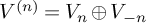 $V^{(n)} = V_n \oplus V_{-n}$
(for
$V^{(n)} = V_n \oplus V_{-n}$
(for
 $n \ne 0$
) and
$n \ne 0$
) and
 $V^{(0)} = V_0$
the indicated subspaces; observe that they also carry (nondegenerate) symmetric bilinear forms.
$V^{(0)} = V_0$
the indicated subspaces; observe that they also carry (nondegenerate) symmetric bilinear forms.
Definition 2.1. For a relatively oriented rank n vector bundle
 $V \to X$
with section
$V \to X$
with section
 $\sigma $
and orientation
$\sigma $
and orientation
 $\rho $
, over a smooth and proper variety
$\rho $
, over a smooth and proper variety
 $f: X \to k$
of dimension n, the Grothendieck–Serre-duality Euler number with respect to
$f: X \to k$
of dimension n, the Grothendieck–Serre-duality Euler number with respect to
 $\sigma $
is
$\sigma $
is
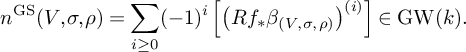 $$\begin{align*}n^{\mathrm{GS}}(V, \sigma, \rho) = \sum_{i \ge 0} (-1)^i \left[\left(Rf_*\beta_{\left(V,\sigma,\rho\right)}\right)^{(i)}\right] \in \mathrm{GW}(k). \end{align*}$$
Remark 2.2. In order not to clutter notation unnecessarily, we also write Definition 2.1 as
 $$\begin{align*}n^{\mathrm{GS}}(V, \sigma, \rho) = \sum_i (-1)^i \left[\left(Rf_*\beta_{\left(V,\sigma,\rho\right)}\right)_i\right]. \end{align*}$$
We shall commit to this kind of abuse of notation from now on.
Recall that
 $n^{\mathrm {GS}}(V, \rho ) \in \mathrm {GW}(k)$
was defined in the introduction in terms of the symmetric bilinear form on
$n^{\mathrm {GS}}(V, \rho ) \in \mathrm {GW}(k)$
was defined in the introduction in terms of the symmetric bilinear form on
 $\bigoplus _{i,j} H^i\left (X, \Lambda ^j V^* \otimes \mathcal L\right )$
.
$\bigoplus _{i,j} H^i\left (X, \Lambda ^j V^* \otimes \mathcal L\right )$
.
Proposition 2.3. For any section
 $\sigma $
, we have
$\sigma $
, we have
 $n^{\mathrm {GS}}(V, \sigma , \rho ) = n^{\mathrm {GS}}(V, \rho ) \in \mathrm {GW}(k)$
.
$n^{\mathrm {GS}}(V, \sigma , \rho ) = n^{\mathrm {GS}}(V, \rho ) \in \mathrm {GW}(k)$
.
To prove Proposition 2.3, we use the hypercohomology spectral sequence
 $E^{i,j}_r(K^{\bullet })$
associated to a complex
$E^{i,j}_r(K^{\bullet })$
associated to a complex
 $K^{\bullet }$
of locally free sheaves on X:
$K^{\bullet }$
of locally free sheaves on X:
 $$ \begin{align*}E^{i,j}_1(K^{\bullet}) : = \mathrm{H}^j\left(X, K^i\right) \Rightarrow R^{i+j} f_* K^{\bullet}.\end{align*} $$
Let
 $F_i$
denote the resulting filtration on
$F_i$
denote the resulting filtration on
 $R^{*} f_* K^{\bullet }$
, such that
$R^{*} f_* K^{\bullet }$
, such that
 $$ \begin{align*}\cdots \supseteq F_i = \mathrm{Im}\left(\mathrm{H}^*\left(X, K^{\bullet \geq i}\right) \to \mathrm{H}^*(X, K^{\bullet})\right) \supseteq F_{i+1} \supseteq \cdots.\end{align*} $$
Given a perfect symmetric pairing of chain complexes
 $\beta : K^{\bullet } \otimes K^{\bullet } \to \omega _{X/k} [n]$
, the cup product induces pairings
$\beta : K^{\bullet } \otimes K^{\bullet } \to \omega _{X/k} [n]$
, the cup product induces pairings
 $$\begin{align*}\beta': R^*f_* K^{\bullet} \otimes R^*f_* K^{\bullet} \to R^*f_* \omega_{X/k} [n] \to k \end{align*}$$
and
 $$\begin{align*}\beta_1: E^{*,*}_1(K^{\bullet}) \otimes E^{*,*}_1(K^{\bullet}) \to k.\end{align*}$$
The following properties hold:
-
(1) Placing the k in the codomain of
$\beta _1$
in bidegree
$(-n,n)$
,
$\beta _1$
is a map of bigraded vector spaces and satisfies the Leibniz rule with respect to
$d_1$
. It thus induces
$\beta _2: E^{*,*}_2(K^{\bullet }) \otimes E^{*,*}_2(K^{\bullet }) \to k$
. Then
$\beta _2$
satisfies the Leibnitz rule with respect to
$d_2$
and hence induces
$\beta _3$
, and so on. -
(2) All the pairings
$\beta _i$
are perfect. -
(3) The pairing
$\beta '$
is compatible with the filtration in the sense that
$\beta '(F_i,F_k) = 0$
if
$i+k>-n$
. -
(4) It follows that
$\beta '$
induces a pairing on
$\mathrm {gr}_{\bullet } R^*f_* K^{\bullet } $
. Under the isomorphism
$\mathrm {gr}_{\bullet } \simeq E_\infty $
, it coincides with
$\beta _\infty $
. -
(5)
$\beta '$
is perfect in the filtered sense: the induced pairing
$F_i \otimes R^*f_* K^{\bullet }/F_{-n-i+1} \to k$
is perfect. (In particular, the pairing
$\beta '$
is perfect.)


Remark 2.4. We do not know a reference for these facts, and proving them would take us too far afield. The main idea is that we have a sequence of duality-preserving functors
 $$\begin{align*}C^{\mathrm{perf}}(X) \xrightarrow{\sigma_{\bullet}} D(X)^{\mathrm{fil}} \xrightarrow{\pi_*} D(k)^{\mathrm{fil}}. \end{align*}$$
Here
 $C^{\mathrm {perf}}(X)$
denotes the category of bounded chain complexes of vector bundles,
$C^{\mathrm {perf}}(X)$
denotes the category of bounded chain complexes of vector bundles,
 $D(X)^{\mathrm {fil}}$
is the filtered derived category [Reference Gwilliam and Pavlov39], and
$D(X)^{\mathrm {fil}}$
is the filtered derived category [Reference Gwilliam and Pavlov39], and
 $\sigma _{\bullet }$
is the ‘stupid truncation’ functor (composed with forgetting to the filtered derived category). The first duality is with respect to
$\sigma _{\bullet }$
is the ‘stupid truncation’ functor (composed with forgetting to the filtered derived category). The first duality is with respect to
 $\underline {\operatorname {Hom}}(\mathord -, \omega [n])$
, the second with respect to
$\underline {\operatorname {Hom}}(\mathord -, \omega [n])$
, the second with respect to
 $\underline {\operatorname {Hom}}(\mathord -, \sigma _{\bullet }(\omega [n])) = \underline {\operatorname {Hom}}(\mathord -, \omega [n](-n))$
, and the third with respect to
$\underline {\operatorname {Hom}}(\mathord -, \sigma _{\bullet }(\omega [n])) = \underline {\operatorname {Hom}}(\mathord -, \omega [n](-n))$
, and the third with respect to
 $\underline {\operatorname {Hom}}(\mathord -, k[0](-n))$
. There are further duality-preserving functors
$\underline {\operatorname {Hom}}(\mathord -, k[0](-n))$
. There are further duality-preserving functors
 $$\begin{align*}(\mathord-)^{\mathrm{gr}}: D(k)^{\mathrm{fil}} \to D(k)^{\mathrm{gr}} \quad \text{and} \quad U: D(k)^{\mathrm{fil}} \to D(k), \end{align*}$$
where
 $D(X)^{\mathrm {gr}} = \mathrm {Fun}(\mathbb {Z}, D(X))$
, with
$D(X)^{\mathrm {gr}} = \mathrm {Fun}(\mathbb {Z}, D(X))$
, with
 $\mathbb {Z}$
viewed as a discrete category. Hence any perfect pairing
$\mathbb {Z}$
viewed as a discrete category. Hence any perfect pairing
 $C \otimes C \to k[0](-n) \in D(k)^{\mathrm {fil}}$
induces a perfect pairing on
$C \otimes C \to k[0](-n) \in D(k)^{\mathrm {fil}}$
induces a perfect pairing on
 $H_*C^{\mathrm {gr}} \otimes H_*C^{\mathrm {gr}} \to k(-n,n)$
, satisfying property (1), and a pairing
$H_*C^{\mathrm {gr}} \otimes H_*C^{\mathrm {gr}} \to k(-n,n)$
, satisfying property (1), and a pairing
 $H_*UC \otimes H_* UC \to k$
, satisfying properties (3) and (5). Moreover there is a spectral sequence
$H_*UC \otimes H_* UC \to k$
, satisfying properties (3) and (5). Moreover there is a spectral sequence
 $E_1 = H_*C^{\mathrm {gr}} \Rightarrow H_* UC$
, satisfying properties (1) and (4). Property (2) is obtained from the fact that passage to homology is a duality-preserving functor.
$E_1 = H_*C^{\mathrm {gr}} \Rightarrow H_* UC$
, satisfying properties (1) and (4). Property (2) is obtained from the fact that passage to homology is a duality-preserving functor.
We apply this to
 $K^{\bullet } \in C^{\mathrm {perf}}(X)$
; then
$K^{\bullet } \in C^{\mathrm {perf}}(X)$
; then
 $\mathrm {gr}_i \sigma _{\bullet } K^{\bullet } = K^i[i]$
and hence
$\mathrm {gr}_i \sigma _{\bullet } K^{\bullet } = K^i[i]$
and hence
 $\mathrm {gr}_i(\pi _*\sigma _{\bullet } K^{\bullet }) = \pi _* K^i[i]$
.
$\mathrm {gr}_i(\pi _*\sigma _{\bullet } K^{\bullet }) = \pi _* K^i[i]$
.
Lemma 2.5. Let X be a graded k-vector space with a finite decreasing filtration
 $$ \begin{align*}X \supset \cdots \supset X_{\bullet} \supset X_{\bullet +1} \supset \cdots.\end{align*} $$
Suppose that
 $X \otimes X \to k$
is a perfect symmetric bilinear pairing, which is compatible with the filtration in the sense of properties (3) and (5). Let
$X \otimes X \to k$
is a perfect symmetric bilinear pairing, which is compatible with the filtration in the sense of properties (3) and (5). Let
 $X^i$
denote the ith graded subspace of X and
$X^i$
denote the ith graded subspace of X and
 $X_{\bullet }^i$
denote the ith graded subspace of
$X_{\bullet }^i$
denote the ith graded subspace of
 $X_{\bullet }$
. Then in
$X_{\bullet }$
. Then in
 $\mathrm {GW}(k)$
, there is an equality
$\mathrm {GW}(k)$
, there is an equality
 $$\begin{align*}\sum_i (-1)^i \left[X^i\right] = \sum_i (-1)^i \left[\mathrm{gr}_{\bullet} X^i\right].\end{align*}$$
Proof. Note that property (5) implies that the pairing
 $\mathrm {gr}_{\bullet } X$
is nondegenerate, so the statement makes sense (recall Remark 2.2). On any graded symmetric bilinear form, the degree i and
$\mathrm {gr}_{\bullet } X$
is nondegenerate, so the statement makes sense (recall Remark 2.2). On any graded symmetric bilinear form, the degree i and
 $-i$
parts for
$-i$
parts for
 $i\ne 0$
assemble into a metabolic space, with Grothendieck–Witt class determined by the rank (see Lemma B.2). It is clear that the ranks on both sides of our equation are the same; hence it suffices to prove the lemma in the case where
$i\ne 0$
assemble into a metabolic space, with Grothendieck–Witt class determined by the rank (see Lemma B.2). It is clear that the ranks on both sides of our equation are the same; hence it suffices to prove the lemma in the case where
 $X^i=0$
for
$X^i=0$
for
 $i \ne 0$
. We may thus ignore the gradings.
$i \ne 0$
. We may thus ignore the gradings.
Let N be maximal with the property that
 $X_N \ne 0$
. We have a perfect pairing
$X_N \ne 0$
. We have a perfect pairing
 $$\begin{align*}X_{N+1} \otimes X/X_{-n-N} \to k. \end{align*}$$
Since
 $X_{N+1}=0$
, we deduce that
$X_{N+1}=0$
, we deduce that
 $X_{-n-N} = X$
and hence
$X_{-n-N} = X$
and hence
 $X_j = X$
for all
$X_j = X$
for all
 $j \le -n-N$
. If
$j \le -n-N$
. If
 $-n-N \ge N$
, then
$-n-N \ge N$
, then
 $X = X_N(N)$
and there is nothing to prove; hence assume the opposite.
$X = X_N(N)$
and there is nothing to prove; hence assume the opposite.
We have the perfect pairing
 $$\begin{align*}X_N/X_{N+1} \otimes X_{-n-N}/X_{-n-N+1} \simeq X_N \otimes X/X_{-n-N+1} \to k. \end{align*}$$
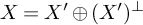
Pick a sequence of subspaces
 $X \supset X^{\prime }_{-n-N+1} \supset \dots \supset X^{\prime }_{N-1}$
such that
$X \supset X^{\prime }_{-n-N+1} \supset \dots \supset X^{\prime }_{N-1}$
such that
 $X^{\prime }_i \subset X_i$
and the canonical projection
$X^{\prime }_i \subset X_i$
and the canonical projection
 $X^{\prime }_i \to X_i/X_{N}$
is an isomorphism. Extend the filtration
$X^{\prime }_i \to X_i/X_{N}$
is an isomorphism. Extend the filtration
 $X'$
by
$X'$
by
 $0$
on the left and constantly on the right. By construction,
$0$
on the left and constantly on the right. By construction,
 $X^{\prime \mathrm {gr}}_i = X^{\mathrm {gr}}_i$
for
$X^{\prime \mathrm {gr}}_i = X^{\mathrm {gr}}_i$
for
 $i \ne N,-n-N$
, and the pairing on
$i \ne N,-n-N$
, and the pairing on
 $X' \subset X$
is perfect in the filtered sense. By [Reference Milnor and Husemoller59, Lemma I.3.1], we have
$X' \subset X$
is perfect in the filtered sense. By [Reference Milnor and Husemoller59, Lemma I.3.1], we have
 $X = X'\oplus (X')^\perp $
. By induction on N, we have
$X = X'\oplus (X')^\perp $
. By induction on N, we have
 $[X'] = [\mathrm {gr}_{\bullet } X']$
. It thus suffices to show that
$[X'] = [\mathrm {gr}_{\bullet } X']$
. It thus suffices to show that
 $\left [(X')^\perp \right ] = [\mathrm {gr}_N X \oplus \mathrm {gr}_{-n-N} X]$
. This holds because both sides are metabolic of the same rank:
$\left [(X')^\perp \right ] = [\mathrm {gr}_N X \oplus \mathrm {gr}_{-n-N} X]$
. This holds because both sides are metabolic of the same rank:
 $X_{-n-N}$
is an isotropic subspace of half rank on either side (see again Lemma B.2).
$X_{-n-N}$
is an isotropic subspace of half rank on either side (see again Lemma B.2).
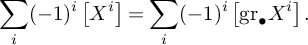
Lemma 2.6. Let
 $E^{\bullet }$
be a chain complex with a nondegenerate, symmetric bilinear form
$E^{\bullet }$
be a chain complex with a nondegenerate, symmetric bilinear form
 $E^{\bullet } \otimes E^{\bullet } \to k[0]$
. Then
$E^{\bullet } \otimes E^{\bullet } \to k[0]$
. Then
 $$\begin{align*}\sum_i (-1)^i \left[H^i(E)\right] = \sum_i \left[E^i\right] \in \mathrm{GW}(k). \end{align*}$$
Proof. Since passing to homology is a duality-preserving functor, the statement makes sense. Both sides have the same rank, so it suffices to prove equality in
 $\mathrm {W}(k)$
(see Lemma B.2). We have a perfect pairing
$\mathrm {W}(k)$
(see Lemma B.2). We have a perfect pairing
 $C^i \otimes C^{-i} \to k$
, and similarly for homology. Both are metabolic unless
$C^i \otimes C^{-i} \to k$
, and similarly for homology. Both are metabolic unless
 $i = 0$
. We can choose a splitting
$i = 0$
. We can choose a splitting
 $$\begin{align*}C^{0} = H \oplus C', \end{align*}$$
where
 $H \subset ker\left (C^{0} \to C^{1}\right )$
maps isomorphically to
$H \subset ker\left (C^{0} \to C^{1}\right )$
maps isomorphically to
 $H^{0}(C)$
. The restriction of the pairing on
$H^{0}(C)$
. The restriction of the pairing on
 $C^{0}$
to H is perfect by construction, and hence
$C^{0}$
to H is perfect by construction, and hence
 $C^{0} = H \oplus H^\perp $
. It suffices to show that
$C^{0} = H \oplus H^\perp $
. It suffices to show that
 $H^\perp $
is metabolic. Compatibility of the pairing with the differential shows that
$H^\perp $
is metabolic. Compatibility of the pairing with the differential shows that
 $d\left (C^{-1}\right ) \subset C^{0}$
is an isotropic subspace. Self-duality shows that
$d\left (C^{-1}\right ) \subset C^{0}$
is an isotropic subspace. Self-duality shows that
 $$\begin{align*}\mathrm{Im}\left(d: C^{-1} \to C^{0}\right) \simeq \mathrm{Im}\left(d^\vee: \left(C^{1}\right)^\vee \to \left(C^{0}\right)^\vee\right) \simeq \mathrm{Im}\left(d: C^{0} \to C^{1}\right)^\vee, \end{align*}$$
which implies that
 $d\left (C^{-1}\right ) \subset H^\perp $
is of half rank. This concludes the proof.
$d\left (C^{-1}\right ) \subset H^\perp $
is of half rank. This concludes the proof.
Proof of Proposition 2.3. Let
 $K^{\bullet } =K(V, \sigma )^{\bullet } \otimes \mathcal L $
. We compute
$K^{\bullet } =K(V, \sigma )^{\bullet } \otimes \mathcal L $
. We compute
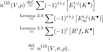 $$ \begin{align*} & n^{\mathrm{GS}}(V, \rho) \stackrel{\text{def.}}{=} \sum (-1)^{i+j} \left[E^{i,j}_1(K^{\bullet})\right] \\ & \qquad \quad \stackrel{\text{Lemma~2.6}}{=} \sum (-1)^{i+j} \left[E^{i,j}_{\infty}(K^{\bullet})\right] \\ & \qquad \quad \stackrel{\text{Lemma~2.5}}{=} \sum_i (-1)^i \left[R^if_* K^{\bullet}\right] \\ & \qquad \qquad \ \stackrel{\text{def.}}{=} n^{\mathrm{GS}}(V, \sigma, \rho). \end{align*} $$
This is the desired result.
Remark 2.7. Admitting a version of Hermitian K-theory which is
 $\mathbb A^1$
-invariant on regular schemes and has proper push-forwards, one can give an alternative proof of Proposition 2.3 by considering the Koszul complex with respect to the section
$\mathbb A^1$
-invariant on regular schemes and has proper push-forwards, one can give an alternative proof of Proposition 2.3 by considering the Koszul complex with respect to the section
 $t\sigma $
on
$t\sigma $
on
 $\mathbb A^1 \times X$
. While we believe such a theory exists, at the time of writing there is no reference for this in characteristic
$\mathbb A^1 \times X$
. While we believe such a theory exists, at the time of writing there is no reference for this in characteristic
 $2$
, so we chose to present our argument instead.
$2$
, so we chose to present our argument instead.
2.2 Local indices for
$n^{\mathrm {GS}}(V, \sigma, \rho )$

Suppose that
 $\sigma $
is a section with only isolated zeros. Let i denote the closed immersion
$\sigma $
is a section with only isolated zeros. Let i denote the closed immersion
 $i: Z = Z(\sigma ) \hookrightarrow X$
given by the zero locus of
$i: Z = Z(\sigma ) \hookrightarrow X$
given by the zero locus of
 $\sigma $
. We express
$\sigma $
. We express
 $n^{\mathrm {GS}}(V, \sigma , \rho )$
as a sum over the points z of Z of a local index at z. To do this, we use a push-forward in a suitable context and show that
$n^{\mathrm {GS}}(V, \sigma , \rho )$
as a sum over the points z of Z of a local index at z. To do this, we use a push-forward in a suitable context and show that
 $\beta _{\left (V,\sigma \right )}$
is a push-forward from Z.
$\beta _{\left (V,\sigma \right )}$
is a push-forward from Z.
For a line bundle
 $\mathcal L$
on a scheme X, denote by
$\mathcal L$
on a scheme X, denote by
 $\mathrm {BL}_{\mathrm {naive}}(D(X), \mathcal L[n])$
the set of isomorphism classes of nondegenerate symmetric bilinear forms on the derived category of perfect complexes on X, with respect to the duality
$\mathrm {BL}_{\mathrm {naive}}(D(X), \mathcal L[n])$
the set of isomorphism classes of nondegenerate symmetric bilinear forms on the derived category of perfect complexes on X, with respect to the duality
 $\underline {\operatorname {Hom}}(\mathord -, \mathcal L[n])$
. For a proper, lci map
$\underline {\operatorname {Hom}}(\mathord -, \mathcal L[n])$
. For a proper, lci map
 $f: X' \to X$
, coherent duality supplies us with a trace map
$f: X' \to X$
, coherent duality supplies us with a trace map
 $\eta _{f,\mathcal L}: f_* f^!(\mathcal L)\to \mathcal L$
. We can use this [Reference Calmès and Hornbostel21, Theorem 4.2.9] to build a push-forward
$\eta _{f,\mathcal L}: f_* f^!(\mathcal L)\to \mathcal L$
. We can use this [Reference Calmès and Hornbostel21, Theorem 4.2.9] to build a push-forward
 $$ \begin{gather*} f_*: \mathrm{BL}_{\mathrm{naive}}\left(D(X'), f^!\mathcal L\right) \to \mathrm{BL}_{\mathrm{naive}}(D(X), \mathcal L), \\ \left[E \otimes E \xrightarrow{\phi} f^! \mathcal L\right] \mapsto \left[f_* E \otimes f_*E \to f_*(E \otimes E) \xrightarrow{f_* \phi} f_*\left(f^! \mathcal L\right) \xrightarrow{\eta_{f,\mathcal L}} \mathcal L\right]. \end{gather*} $$
Remark 2.8. There is a canonical weak equivalence
 $f^!\mathcal L \simeq f^! \mathcal O_X \otimes f^* \mathcal L$
, and
$f^!\mathcal L \simeq f^! \mathcal O_X \otimes f^* \mathcal L$
, and
 $\eta _{f,\mathcal L}$
is given by the composition
$\eta _{f,\mathcal L}$
is given by the composition
 $$ \begin{align*}f_*\left(f^!\mathcal L\right) \simeq f_*\left( f^! \mathcal O_X \otimes f^* \mathcal L \right) \simeq f_* f^! \mathcal O_X \otimes \mathcal L \xrightarrow{\eta_f \otimes \operatorname{id}_{\mathcal L}} \mathcal L,\end{align*} $$
where
 $\eta _f = \eta _{f, \mathcal O_S}$
[73, Lemma 47.17.8].
$\eta _f = \eta _{f, \mathcal O_S}$
[73, Lemma 47.17.8].
Example 2.9. Consider the case of a relatively oriented vector bundle V on a smooth, proper variety
 $f: X \to \operatorname {Spec}(k)$
. Note that elements of
$f: X \to \operatorname {Spec}(k)$
. Note that elements of
 $\mathrm {BL}^{\mathrm {naive}}(k)$
are just isomorphism classes of symmetric bilinear forms on graded vector spaces. The orientation supplies us with an equivalence
$\mathrm {BL}^{\mathrm {naive}}(k)$
are just isomorphism classes of symmetric bilinear forms on graded vector spaces. The orientation supplies us with an equivalence
 $$\begin{align*}f^!(\mathcal O_k) \simeq \omega_{X/k}[n] \simeq \det V^* [n] \otimes \mathcal L^{\otimes 2}. \end{align*}$$
Under the induced push-forward map we have
 $$\begin{align*}f_* \left[\beta_{\left(V,\sigma,\rho\right)}\right] = n^{\mathrm{GS}}(V, \sigma, \rho) \in \mathrm{BL}^{\mathrm{naive}}(k), \end{align*}$$
where
 $\beta _{\left (V,\sigma ,\rho \right )} \in \mathrm {BL}^{\mathrm {naive}}\left (X, \det V^* [n] \otimes \mathcal L^{\otimes 2}\right )$
is the form on
$\beta _{\left (V,\sigma ,\rho \right )} \in \mathrm {BL}^{\mathrm {naive}}\left (X, \det V^* [n] \otimes \mathcal L^{\otimes 2}\right )$
is the form on
 $K(V, \sigma ) \otimes \mathcal L$
defined in §2.1.
$K(V, \sigma ) \otimes \mathcal L$
defined in §2.1.
Remark 2.10. A symmetric bilinear form
 $\phi $
on the derived category
$\phi $
on the derived category
 $D(S)$
is usually not a very sensible notion. We offer three ways around this:
$D(S)$
is usually not a very sensible notion. We offer three ways around this:
-
(1) If
$1/2 \in S$
, we could look at the image of
$\phi $
in the Balmer–Witt group of S. -
(2) If
$\phi $
happens to be concentrated in degree
$0$
, it corresponds to a symmetric bilinear form on a vector bundle on S, which is a sensible invariant. -
(3) If
$S = \operatorname {Spec}(k)$
is the spectrum of a field, then
$D(S)$
is equivalent to the category of graded vector spaces, and we can split
$\phi $
into components by degree and consider
$$\begin{align*}cl(\phi) := \left[H^0(\phi)\right] + \sum_{i> 0} (-1)^i \left[H^i(\phi) \oplus H^{-i}(\phi)\right] \in \mathrm{GW}(k). \end{align*}$$


Let
 $1_Z$
denote the element of
$1_Z$
denote the element of
 $\mathrm {BL}_{\mathrm {naive}}(D(Z), \mathcal O_Z[0])$
represented by
$\mathrm {BL}_{\mathrm {naive}}(D(Z), \mathcal O_Z[0])$
represented by
 $\mathcal {O}_Z \otimes \mathcal {O}_Z \to \mathcal {O}_Z$
.
$\mathcal {O}_Z \otimes \mathcal {O}_Z \to \mathcal {O}_Z$
.
Proposition 2.11. Let X be a scheme, V a vector bundle, and
 $\sigma \in \Gamma (X, V)$
a section locally given by a regular sequence. Write
$\sigma \in \Gamma (X, V)$
a section locally given by a regular sequence. Write
 $i: Z = Z(\sigma ) \hookrightarrow X$
for the inclusion of the zero scheme. Proposition B.1 yields a canonical equivalence
$i: Z = Z(\sigma ) \hookrightarrow X$
for the inclusion of the zero scheme. Proposition B.1 yields a canonical equivalence
 $i^!\det (V^*)[n] \simeq \mathcal O_Z[0]$
, where n is the rank of V; under the induced map
$i^!\det (V^*)[n] \simeq \mathcal O_Z[0]$
, where n is the rank of V; under the induced map
 $$\begin{align*}i_*: \mathrm{BL}_{\mathrm{naive}}(D(Z), \mathcal O_Z[0]) \to \mathrm{BL}_{\mathrm{naive}}(D(X), \det(V^*)[n]), \end{align*}$$
we have
 $i_*(1_Z) = \beta _{\left (V,\sigma \right )}$
, where
$i_*(1_Z) = \beta _{\left (V,\sigma \right )}$
, where
 $$\begin{align*}\beta_{\left(V,\sigma\right)}: K(V, \sigma) \otimes K(V, \sigma) \to \det(V^*)[n] \end{align*}$$
is the canonical pairing on the Koszul complex as in §2.1.
Proof. Because
 $\sigma $
locally corresponds to a regular sequence, the canonical map
$\sigma $
locally corresponds to a regular sequence, the canonical map
 $r:K(V, \sigma )^{\bullet } \to i_*\mathcal {O}_Z$
is an equivalence in
$r:K(V, \sigma )^{\bullet } \to i_*\mathcal {O}_Z$
is an equivalence in
 $D(X)$
. The canonical projection
$D(X)$
. The canonical projection
 $i_* \mathcal O_Z \simeq K(V, \sigma ) \to \det (V^*)[n]$
induces by adjunction a map
$i_* \mathcal O_Z \simeq K(V, \sigma ) \to \det (V^*)[n]$
induces by adjunction a map
 $\mathcal O_Z \to i^!\det (V^*)[n]$
. We claim that this is the equivalence of Proposition B.1. The proof of that proposition shows that the problem is local on Z, so we may assume that V is trivial. Then this map is precisely the isomorphism constructed in [Reference Hartshorne40, Proposition III.7.2 and preceeding pages], which is also the isomorphism used in the proof of Proposition B.1.
$\mathcal O_Z \to i^!\det (V^*)[n]$
. We claim that this is the equivalence of Proposition B.1. The proof of that proposition shows that the problem is local on Z, so we may assume that V is trivial. Then this map is precisely the isomorphism constructed in [Reference Hartshorne40, Proposition III.7.2 and preceeding pages], which is also the isomorphism used in the proof of Proposition B.1.
Now we prove that
 $i_*(1_Z) = \beta _{\left (V,\sigma \right )}$
. Consider the following diagram:
$i_*(1_Z) = \beta _{\left (V,\sigma \right )}$
. Consider the following diagram:

The map
 $m_K: K(V, \sigma ) \otimes K(V, \sigma ) \to K(V, \sigma )$
is the canonical multiplication (see §2.1, property (2)) and
$m_K: K(V, \sigma ) \otimes K(V, \sigma ) \to K(V, \sigma )$
is the canonical multiplication (see §2.1, property (2)) and
 $m_Z: i_*\mathcal O_Z \otimes ^L i_* \mathcal O_Z \to i_* \mathcal O_Z \otimes i_* \mathcal O_Z \to i_* \mathcal O_Z$
is equivalently given by either multiplication in
$m_Z: i_*\mathcal O_Z \otimes ^L i_* \mathcal O_Z \to i_* \mathcal O_Z \otimes i_* \mathcal O_Z \to i_* \mathcal O_Z$
is equivalently given by either multiplication in
 $\mathcal O_Z$
or the lax monoidal witness transformation of
$\mathcal O_Z$
or the lax monoidal witness transformation of
 $i_*$
. The former interpretation shows that the left-hand square commutes. The pairing
$i_*$
. The former interpretation shows that the left-hand square commutes. The pairing
 $i_*(1)$
is given by the composite from the top right corner to the bottom right corner. To prove the claim, it suffices to show that the bottom-row composite
$i_*(1)$
is given by the composite from the top right corner to the bottom right corner. To prove the claim, it suffices to show that the bottom-row composite
 $K(V, \sigma ) \to \det (V^*)[n]$
is the canonical projection. This follows by adjunction from our choice of equivalence
$K(V, \sigma ) \to \det (V^*)[n]$
is the canonical projection. This follows by adjunction from our choice of equivalence
 $\mathcal O_Z \simeq i^! \det (V^*)[n]$
.
$\mathcal O_Z \simeq i^! \det (V^*)[n]$
.
This concludes the proof.
Proposition 2.11 is an example of a more general phenomenon given in Meta-Theorem 3.9.
Lemma 2.12 [Reference Calmès and Hornbostel21]
Let
 $g: Z \to Y$
and
$g: Z \to Y$
and
 $f: Y \to X$
be proper maps.Footnote 4 Given equivalences
$f: Y \to X$
be proper maps.Footnote 4 Given equivalences
 $f^! \mathcal L \simeq \mathcal M [n]$
and
$f^! \mathcal L \simeq \mathcal M [n]$
and
 $g^! \mathcal M [n] \simeq \mathcal N$
, the canonical equivalence
$g^! \mathcal M [n] \simeq \mathcal N$
, the canonical equivalence
 $(f g)^! \simeq g^! f^!$
produces a weak equivalence
$(f g)^! \simeq g^! f^!$
produces a weak equivalence
 $(f g)^! \mathcal L \simeq \mathcal N$
, and consequently push-forward maps
$(f g)^! \mathcal L \simeq \mathcal N$
, and consequently push-forward maps
 $$\begin{align*}g_*: \mathrm{BL}_{\mathrm{naive}}(D(Z), \mathcal N) \to \mathrm{BL}_{\mathrm{naive}}(D(Y), \mathcal M [n]), \end{align*}$$
 $$\begin{align*}f_*: \mathrm{BL}_{\mathrm{naive}}(D(Y), \mathcal M [n]) \to \mathrm{BL}_{\mathrm{naive}}(D(X), \mathcal L), \end{align*}$$
 $$\begin{align*}(f g)_*: \mathrm{BL}_{\mathrm{naive}}(D(Z), \mathcal N) \to \mathrm{BL}_{\mathrm{naive}}(D(X), \mathcal L). \end{align*}$$
There is a canonical equivalence
 $(f g)_* \simeq f_* g_*$
.
$(f g)_* \simeq f_* g_*$
.
Proof. The main point is that
 $\eta _{f, \mathcal L} \circ f_*\left (\eta _{g, \mathcal M [n]}\right ) = \eta _{fg, \mathcal L}$
. The categorical details are worked out in the reference.
$\eta _{f, \mathcal L} \circ f_*\left (\eta _{g, \mathcal M [n]}\right ) = \eta _{fg, \mathcal L}$
. The categorical details are worked out in the reference.
Now we get back to our Euler numbers. Let
 $X/k$
be smooth and proper, V a relatively oriented vector bundle, and
$X/k$
be smooth and proper, V a relatively oriented vector bundle, and
 $\sigma $
a section of V with only isolated zeros. Write
$\sigma $
a section of V with only isolated zeros. Write
 $i: Z = Z(\sigma ) \hookrightarrow X$
for the inclusion of the zero scheme of
$i: Z = Z(\sigma ) \hookrightarrow X$
for the inclusion of the zero scheme of
 $\sigma $
. Let
$\sigma $
. Let
 $\varpi : Z \to \operatorname {Spec} k$
and
$\varpi : Z \to \operatorname {Spec} k$
and
 $f: X \to \operatorname {Spec} k$
denote the structure maps, so that
$f: X \to \operatorname {Spec} k$
denote the structure maps, so that
 $\varpi = f i $
.
$\varpi = f i $
.
The weak equivalence
 $i^!\det (V^*)[n] \simeq \mathcal O_Z[0]$
of Proposition 2.11, with Remark 2.8, produces a weak equivalence
$i^!\det (V^*)[n] \simeq \mathcal O_Z[0]$
of Proposition 2.11, with Remark 2.8, produces a weak equivalence
 $i^! \left (\det V^*[n] \otimes \mathcal L^{\otimes 2}\right ) \cong i^* \mathcal L^{\otimes 2}$
. The orientation
$i^! \left (\det V^*[n] \otimes \mathcal L^{\otimes 2}\right ) \cong i^* \mathcal L^{\otimes 2}$
. The orientation
 $\rho $
gives an isomorphism
$\rho $
gives an isomorphism
 $\det V^*[n] \otimes \mathcal L^{\otimes 2}\cong \omega _{X/k}[n]$
. Combining, we have a chosen weak equivalence
$\det V^*[n] \otimes \mathcal L^{\otimes 2}\cong \omega _{X/k}[n]$
. Combining, we have a chosen weak equivalence
 $$\begin{align*}i^! (\omega_{X/k}[n]) \cong i^* \mathcal L^{\otimes 2}. \end{align*}$$
Since also
 $f^! \mathcal {O}_k \simeq \omega _{X/k} [n]$
(see, e.g., Proposition B.1), we therefore obtain a canonical equivalence
$f^! \mathcal {O}_k \simeq \omega _{X/k} [n]$
(see, e.g., Proposition B.1), we therefore obtain a canonical equivalence
 $$\begin{align*}\varpi^! \mathcal{O}_k \simeq i^* \mathcal L^{\otimes 2}. \end{align*}$$
We use this equivalence to define
 $$\begin{align*}\varpi_*: \mathrm{BL}^{\mathrm{naive}}\left(Z, i^* \mathcal L^{\otimes 2}\right) \to \mathrm{BL}^{\mathrm{naive}}(k). \end{align*}$$
Corollary 2.13. With this notation, we have
 $$\begin{align*}n^{\mathrm{GS}}(V, \sigma, \rho) =\varpi_* \left(i^* \mathcal L \otimes i^* \mathcal L \to i^* \mathcal L^{\otimes 2}\right). \end{align*}$$
Proof. By Lemma 2.12 we have
 $\varpi _* = f_* i_*$
. Proposition 2.11 and the projection formula imply that
$\varpi _* = f_* i_*$
. Proposition 2.11 and the projection formula imply that
 $i_*\left (i^* \mathcal L \otimes i^* \mathcal L \to i^* \mathcal L^{\otimes 2}\right ) = \beta _{V,\sigma ,\rho }$
. We conclude by Example 2.9.
$i_*\left (i^* \mathcal L \otimes i^* \mathcal L \to i^* \mathcal L^{\otimes 2}\right ) = \beta _{V,\sigma ,\rho }$
. We conclude by Example 2.9.
Suppose that
 $\sigma $
has isolated zeros, or in other words that the support of
$\sigma $
has isolated zeros, or in other words that the support of
 $\sigma $
is a disjoint union of points. Then
$\sigma $
is a disjoint union of points. Then
 $n^{\mathrm {GS}}(V, \sigma , \rho )$
can be expressed as a sum of local contributions. Namely, for each point z of Z, let
$n^{\mathrm {GS}}(V, \sigma , \rho )$
can be expressed as a sum of local contributions. Namely, for each point z of Z, let
 $i_z: Z_z \hookrightarrow X$
denote the chosen immersion coming from the connected component of Z given by z. Let
$i_z: Z_z \hookrightarrow X$
denote the chosen immersion coming from the connected component of Z given by z. Let
 $\varpi _z: Z_z \to \operatorname {Spec} k$
denote the structure map. Then
$\varpi _z: Z_z \to \operatorname {Spec} k$
denote the structure map. Then
 $$ \begin{align*}n^{\mathrm{GS}}(V, \sigma, \rho) = \sum_{z \in Z}\varpi_{z*} \left(i_z^* \mathcal L \otimes i_z^* \mathcal L \to i_z^* \mathcal L^{\otimes 2}\right) .\end{align*} $$
In light of this we propose the following:
Definition 2.14. For a relatively oriented vector bundle with a section as described, and
 $z \in Z(\sigma )$
, we define
$z \in Z(\sigma )$
, we define
 $$\begin{align*}\mathrm{ind}_z(\sigma) = \mathrm{ind}_z(V, \sigma, \rho) = \varpi_{z*}\left(i_z^* \mathcal L \otimes i_z^* \mathcal L \to i_z^* \mathcal L^{\otimes 2}\right) \in \mathrm{BL}^{\mathrm{naive}}(k). \end{align*}$$
The previous formula then reads
 $$ \begin{align} n^{\mathrm{GS}}(V, \sigma, \rho) = \sum_{z \in Z} \mathrm{ind}_z(V, \sigma, \rho). \end{align} $$
In the next two subsections, we compute the local contributions
 $\mathrm {ind}_z(\sigma )$
as an explicit bilinear form constructed by Scheja and Storch [Reference Scheja and Storch67], appearing in the Eisenbud–Levine–Khimshiashvili signature theorem [Reference Eisenbud and Levine29] and used as the local index of the Euler class constructed in [Reference Kass and Wickelgren49, Section 4].
$\mathrm {ind}_z(\sigma )$
as an explicit bilinear form constructed by Scheja and Storch [Reference Scheja and Storch67], appearing in the Eisenbud–Levine–Khimshiashvili signature theorem [Reference Eisenbud and Levine29] and used as the local index of the Euler class constructed in [Reference Kass and Wickelgren49, Section 4].
2.3 Scheja–Storch and coherent duality
Let S be a scheme,
 $\pi : X \to S$
a smooth scheme of relative dimension n, and
$\pi : X \to S$
a smooth scheme of relative dimension n, and
 $Z \subset X$
closed with
$Z \subset X$
closed with
 $\varpi : Z \to S$
finite. Suppose the following data:
$\varpi : Z \to S$
finite. Suppose the following data:
-
(1) sections
$T_1, \dots , T_n \in \mathcal O(X)$
such that
$T_i \otimes 1 - 1 \otimes T_i$
generate the ideal of
$X \subset X \times _S X$
; -
(2) sections
$f_1, \dots , f_n \in \mathcal O(X)$
such that
$Z = Z(f_1, \dots , f_n)$
.


Remark 2.15. Since
 $Z \to X$
is quasi-finite, Lemma B.5 shows that
$Z \to X$
is quasi-finite, Lemma B.5 shows that
 $f_1, \dots , f_n$
is a regular sequence and
$f_1, \dots , f_n$
is a regular sequence and
 $Z \to X$
is flat, so finite locally free (being finite and finitely presented [73, Tag 02KB]).
$Z \to X$
is flat, so finite locally free (being finite and finitely presented [73, Tag 02KB]).
Choose
 $a_{ij} \in \mathcal O(X \times _S X)$
such that
$a_{ij} \in \mathcal O(X \times _S X)$
such that
 $$\begin{align*}f_i\otimes 1 - 1 \otimes f_i = \sum_j a_{ij}\left(T_j \otimes 1 - 1 \otimes T_j\right). \end{align*}$$
Let
 $\Delta \in \mathcal O(Z \times _S Z)$
be the image of the determinant of
$\Delta \in \mathcal O(Z \times _S Z)$
be the image of the determinant of
 $a_{ij}$
. Since
$a_{ij}$
. Since
 $\varpi $
is finite locally free,
$\varpi $
is finite locally free,
 $\Delta $
determines an element
$\Delta $
determines an element
 $\tilde \Delta $
of
$\tilde \Delta $
of
 $$\begin{align*}\operatorname{Hom}_{\mathcal O_S}\left(\mathcal O_S, (\varpi \times_S \varpi)_* \mathcal O_{Z \times_S Z}\right) \simeq \operatorname{Hom}_{\mathcal O_S}(\mathcal O_S, \varpi_* \mathcal O_Z \otimes \varpi_* \mathcal O_Z) \simeq \operatorname{Hom}_{\mathcal O_S}((\varpi_* \mathcal O_Z)^*, \varpi_* \mathcal O_Z). \end{align*}$$
Remark 2.16. We can make
 $\tilde \Delta $
explicit: if
$\tilde \Delta $
explicit: if
 $\Delta = \sum _i b_i \otimes b_i^{\prime }$
, then
$\Delta = \sum _i b_i \otimes b_i^{\prime }$
, then
 $$\begin{align*}\tilde\Delta(\alpha) = \sum_i \alpha(b_i)b_i^{\prime}. \end{align*}$$
Remark 2.17. By construction, the pullback of
 $\Delta $
along the diagonal
$\Delta $
along the diagonal
 $\delta : Z \to Z \times _S Z$
is the determinant of the differentiation map
$\delta : Z \to Z \times _S Z$
is the determinant of the differentiation map
 $C_{Z/X} \to \Omega _X\rvert _Z$
with respect to the canonical bases. In other words,this is the Jacobian:
$C_{Z/X} \to \Omega _X\rvert _Z$
with respect to the canonical bases. In other words,this is the Jacobian:
 $$\begin{align*}\delta^*(\Delta) = \mathrm{Jac} F := \det \left(\frac{\partial f_i}{\partial T_j}\right)_{i,j=1}^n. \end{align*}$$
Theorem 2.18. Under the foregoing assumptions, the map
 $$\begin{align*}\tilde\Delta: (\varpi_* \mathcal O_Z)^* \to \varpi_* \mathcal O_Z \end{align*}$$
is a symmetric isomorphism and hence determines a symmetric bilinear structure on
 $\varpi _* \mathcal O_Z$
. This is the same structure as
$\varpi _* \mathcal O_Z$
. This is the same structure as
 $\varpi _*(1)$
–that is,
$\varpi _*(1)$
–that is,
 $$\begin{align*}\varpi_*(\mathcal O_Z) \otimes \varpi_*(\mathcal O_Z) \to \varpi_*(\mathcal O_Z) \simeq \varpi_*\left(\varpi^! \mathcal O_S\right) \xrightarrow{\eta_\varpi} \mathcal O_S. \end{align*}$$
Here the isomorphism
 $\varpi ^! \mathcal O_Z \simeq \mathcal O_Z$
arises from
$\varpi ^! \mathcal O_Z \simeq \mathcal O_Z$
arises from
 $$\begin{align*}\varpi^!(\mathcal O_Z) \simeq \widetilde\det L_\varpi \simeq \omega_{Z/X} \otimes \omega_{X/S} \simeq \mathcal O, \end{align*}$$
with the first isomorphism given by Proposition B.1 and the third given by the sections
 $(T_i)$
and
$(T_i)$
and
 $(f_i)$
.
$(f_i)$
.
Remark 2.19. The theorem asserts in particular that the isomorphism
 $\tilde \Delta $
, and hence the section
$\tilde \Delta $
, and hence the section
 $\Delta $
, is independent of the choice of the
$\Delta $
, is independent of the choice of the
 $a_{ij}$
.
$a_{ij}$
.
We begin with some preliminary observations before delving into the proof. The problem is local on S, so we may assume that
 $S = \operatorname {Spec}(A)$
; then
$S = \operatorname {Spec}(A)$
; then
 $Z = \operatorname {Spec}(B)$
. Since
$Z = \operatorname {Spec}(B)$
. Since
 $\varpi $
is finite, there is a canonical isomorphism [Reference Hartshorne40, III §8 Theorem 8.7 (3), or Ideal Theorem (3) p. 6]
$\varpi $
is finite, there is a canonical isomorphism [Reference Hartshorne40, III §8 Theorem 8.7 (3), or Ideal Theorem (3) p. 6]
 $$\begin{align*}\varpi^! \simeq \underline{\operatorname{Hom}}_A(B, \mathord-): D(A) \to D(B). \end{align*}$$
In particular,
 $$\begin{align*}\varpi^!(A) \simeq \underline{\operatorname{Hom}}_A(B, A) \end{align*}$$
and the trace map takes the form [Reference Hartshorne40, Ideal theorem 3) pg 7]
 $$\begin{align*}\varpi_* \varpi^! A \simeq \operatorname{Hom}_A(B, A) \to A, \eta \mapsto \eta(1). \end{align*}$$
Proof of Theorem 2.18. The isomorphisms
 $$\begin{align*}B^* = \underline{\operatorname{Hom}}_A(B,A) \simeq \varpi^!(A) \simeq B \end{align*}$$
determine an element
 $\Delta ^{\prime } \in \operatorname {Hom}_A(B^*, B)$
. The theorem is equivalent to showing that
$\Delta ^{\prime } \in \operatorname {Hom}_A(B^*, B)$
. The theorem is equivalent to showing that
 $\tilde \Delta = \Delta ^{\prime }$
.
$\tilde \Delta = \Delta ^{\prime }$
.
We thus need to make explicit the isomorphism
 $$\begin{align*}\underline{\operatorname{Hom}}_A(B, A) \simeq \varpi^!(\mathcal O_A) \simeq i^! \pi^! (\mathcal O_A) \simeq \omega_{Z/X} \otimes \omega_{X} \simeq \mathcal O. \end{align*}$$
Tracing through the definitions (including the proof of [Reference Hartshorne40, III Proposition 8.2]), one finds that this isomorphism arises by computing
 $$\begin{align*}\operatorname{Ext}^n_X(B, \mathcal O_X) \end{align*}$$
in two ways. One the one hand, the kernel of the surjection
 $\mathcal O_X \to B$
is generated by
$\mathcal O_X \to B$
is generated by
 $f_1, \dots , f_n$
, which is a regular sequence by Remark 2.15; let
$f_1, \dots , f_n$
, which is a regular sequence by Remark 2.15; let
 $K_A(f)^{\bullet }$
denote the corresponding Koszul complex. On the other hand, we can consider the embedding
$K_A(f)^{\bullet }$
denote the corresponding Koszul complex. On the other hand, we can consider the embedding
 $Z \hookrightarrow X \times Z$
; its ideal is generated by the strongly regular sequence
$Z \hookrightarrow X \times Z$
; its ideal is generated by the strongly regular sequence
 $T_i - t_i$
, where
$T_i - t_i$
, where
 $t_i$
is the image of
$t_i$
is the image of
 $T_i$
in B. We thus obtain a resolution
$T_i$
in B. We thus obtain a resolution
 $K_B(T-t)^{\bullet } \to B$
over
$K_B(T-t)^{\bullet } \to B$
over
 $X \times Z$
. Since
$X \times Z$
. Since
 $p: X \times Z \to X$
is finite,
$p: X \times Z \to X$
is finite,
 $p_*K_B(T-t)^{\bullet } \to p_*B=B$
is still a resolution. We shall conflate
$p_*K_B(T-t)^{\bullet } \to p_*B=B$
is still a resolution. We shall conflate
 $K_B(T-t)$
and
$K_B(T-t)$
and
 $p_* K_B(T-t)$
notationally. We can thus compute
$p_* K_B(T-t)$
notationally. We can thus compute
 $$\begin{align*}\operatorname{Ext}^n_{X}(B, \mathcal O_X) \simeq coker\left(\operatorname{Hom}_{X}\left(K_B(T-t)^{n-1}, \mathcal O_X\right) \to \operatorname{Hom}_{X}(K_B(T-t)^{n}, \mathcal O_X)\right). \end{align*}$$
Since
 $\operatorname {Hom}_{X}(B \otimes \mathcal O_X, \mathcal O_X) \simeq \operatorname {Hom}_A(B, \mathcal O_X) \simeq \operatorname {Hom}_A(B, A) \otimes _A \mathcal O_X,$
there is a natural map
$\operatorname {Hom}_{X}(B \otimes \mathcal O_X, \mathcal O_X) \simeq \operatorname {Hom}_A(B, \mathcal O_X) \simeq \operatorname {Hom}_A(B, A) \otimes _A \mathcal O_X,$
there is a natural map
 $\xi : \operatorname {Hom}_A(B, A) \to \operatorname {Hom}_{X}(K_B(T-t)^{n}, \mathcal O_X)$
(sending
$\xi : \operatorname {Hom}_A(B, A) \to \operatorname {Hom}_{X}(K_B(T-t)^{n}, \mathcal O_X)$
(sending
 $\alpha $
to
$\alpha $
to
 $\alpha \otimes 1$
). One checks that this induces
$\alpha \otimes 1$
). One checks that this induces
 $\operatorname {Hom}_A(B, A) \simeq coker(\dots ) \simeq \operatorname {Ext}^n_{X}(B, \mathcal O_X)$
.
$\operatorname {Hom}_A(B, A) \simeq coker(\dots ) \simeq \operatorname {Ext}^n_{X}(B, \mathcal O_X)$
.
We can write down a map of resolutions
 $\zeta : K_A(f) \to K_B(T-t)$
as follows: The kernel of
$\zeta : K_A(f) \to K_B(T-t)$
as follows: The kernel of
 $B \otimes \mathcal O_X \to B$
is by construction generated by
$B \otimes \mathcal O_X \to B$
is by construction generated by
 $\{T_i - t_i\}_i$
, but it also contains
$\{T_i - t_i\}_i$
, but it also contains
 $f_i$
. Note that
$f_i$
. Note that
 $f_i = \sum _j \bar a_{ij}\left (T_j - t_j\right )$
, where we write
$f_i = \sum _j \bar a_{ij}\left (T_j - t_j\right )$
, where we write
 $\bar a_{ij}$
for the image of
$\bar a_{ij}$
for the image of
 $a_{ij}$
in
$a_{ij}$
in
 $\mathcal O_X \otimes B$
. Letting
$\mathcal O_X \otimes B$
. Letting
 $K_A(f)$
be the exterior algebra on
$K_A(f)$
be the exterior algebra on
 $\{e_1, \dots , e_n\}$
and
$\{e_1, \dots , e_n\}$
and
 $K_B(T-t)$
the exterior algebra on
$K_B(T-t)$
the exterior algebra on
 $\left \{e_1^{\prime }, \dots , e_n^{\prime }\right \}$
, the map
$\left \{e_1^{\prime }, \dots , e_n^{\prime }\right \}$
, the map
 $\zeta $
is specified by
$\zeta $
is specified by
 $\zeta (e_i) = \sum _j \bar a_{ij} e_j^{\prime }$
. The isomorphism
$\zeta (e_i) = \sum _j \bar a_{ij} e_j^{\prime }$
. The isomorphism
 $$\begin{align*}\operatorname{Hom}_A(B, A) \simeq h^n \operatorname{Hom}_{X}(K_B(T-t)^{\bullet}, \mathcal O_X) \simeq h^n \operatorname{Hom}_{X}(K_A(f)^{\bullet}, \mathcal O_X) \simeq B \end{align*}$$
is thus given by
 $$ \begin{gather*} \operatorname{Hom}_A(B, A) \xrightarrow{\xi} \operatorname{Hom}_{X}(K_B(T-t)^{n}, \mathcal O_X) \xrightarrow{\det\left(a_{ij}\right)^*} \operatorname{Hom}_{X}(K_A(f)^{n}, \mathcal O_X) \\ \simeq \operatorname{Hom}_{X}(\mathcal O_X, \mathcal O_X) \simeq \mathcal O_X \to B. \end{gather*} $$
Write the image of
 $\det (a_{ij})$
in
$\det (a_{ij})$
in
 $B \otimes B$
as
$B \otimes B$
as
 $\sum _k b_k \otimes b_k^{\prime }$
. Tracing through the definitions, we find that this composite sends
$\sum _k b_k \otimes b_k^{\prime }$
. Tracing through the definitions, we find that this composite sends
 $\alpha \in \operatorname {Hom}_A(B, A)$
to
$\alpha \in \operatorname {Hom}_A(B, A)$
to
 $\sum _k \alpha (b_k)b_k^{\prime }$
. By Remark 2.16, this is precisely
$\sum _k \alpha (b_k)b_k^{\prime }$
. By Remark 2.16, this is precisely
 $\tilde \Delta $
.
$\tilde \Delta $
.
This concludes the proof.□
Definition 2.20. If
 $X=U \subset \mathbb A^n_S$
,
$X=U \subset \mathbb A^n_S$
,
 $(T_i)$
are the standard coordinates, and
$(T_i)$
are the standard coordinates, and
 $F=(f_1, \dots , f_n)$
, we denote the symmetric bilinear form already constructed by
$F=(f_1, \dots , f_n)$
, we denote the symmetric bilinear form already constructed by
 $$\begin{align*}\langle - \vert - \rangle^{\mathrm{SS}} = \langle - \vert - \rangle^{\mathrm{SS}}(U, F, S). \end{align*}$$
This form was first constructed, without explicitly using coherent duality, by Scheja and Storch [Reference Ananyevskiy2, Reference Scheja and Storch67].
Example 2.21. Suppose that
 $Z \to S$
is an isomorphism (where
$Z \to S$
is an isomorphism (where
 $Z=Z(F)$
as before, so that the diagonal
$Z=Z(F)$
as before, so that the diagonal
 $\delta : Z \to Z \times _S Z$
is also an isomorphism. Then
$\delta : Z \to Z \times _S Z$
is also an isomorphism. Then
 $\langle - \vert - \rangle ^{\mathrm {SS}}$
is just the rank
$\langle - \vert - \rangle ^{\mathrm {SS}}$
is just the rank
 $1$
bilinear form corresponding to multiplication by
$1$
bilinear form corresponding to multiplication by
 $\delta ^*(\Delta ) \in \mathcal O_Z \simeq \mathcal O_S$
. In other words, using Remark 2.17,
$\delta ^*(\Delta ) \in \mathcal O_Z \simeq \mathcal O_S$
. In other words, using Remark 2.17,
 $\langle - \vert - \rangle ^{\mathrm {SS}}$
identifies with
$\langle - \vert - \rangle ^{\mathrm {SS}}$
identifies with
 $(x,y) \mapsto (\mathrm {Jac} F) xy$
.
$(x,y) \mapsto (\mathrm {Jac} F) xy$
.
2.4 The Poincaré–Hopf Euler number with respect to a section
In this subsection, we recall the Euler class defined in [Reference Kass and Wickelgren49, Section 4] and prove Theorem 1.1. To distinguish this Euler class from the others under consideration, here we call it the Poincaré–Hopf Euler number, because it is a sum of local indices as in the Poincaré–Hopf theorem for the Euler characteristic of a manifold. It is defined using local coordinates.
Let k be a field, and let X be an n-dimensional smooth k-scheme. Let z be a closed point of X.
Definition 2.22 compare [Reference Kass and Wickelgren49, Definition 17]
By a system of Nisnevich coordinates around z we mean a Zariski open neighborhood U of z in X, and an étale map
 $\varphi : U \to \mathbb A^n_k$
such that the extension of residue fields
$\varphi : U \to \mathbb A^n_k$
such that the extension of residue fields
 $k(\varphi (z)) \subseteq k(z)$
is an isomorphism.
$k(\varphi (z)) \subseteq k(z)$
is an isomorphism.
Proposition 2.23. When
 $n>0$
, there exists a system of Nisnevich coordinates around every closed point z of X.
$n>0$
, there exists a system of Nisnevich coordinates around every closed point z of X.
Proof. When k is infinite, this follows from [Reference Knus52, Chapter 8. Proposition 3.2.1]. When
 $k(z)/k$
is separable, for instance when k is finite, this is [Reference Kass and Wickelgren49, Lemma 18].
$k(z)/k$
is separable, for instance when k is finite, this is [Reference Kass and Wickelgren49, Lemma 18].
As before, let V be a relatively oriented, rank n vector bundle on X. Let
 $\sigma $
be a section with only isolated zeros, and let
$\sigma $
be a section with only isolated zeros, and let
 $Z \hookrightarrow X$
denote the closed subscheme given by the zero locus of
$Z \hookrightarrow X$
denote the closed subscheme given by the zero locus of
 $\sigma $
. Let z be a point of Z. The Poincaré–Hopf local index or degree
$\sigma $
. Let z be a point of Z. The Poincaré–Hopf local index or degree
 $$ \begin{align*}\mathrm{ind}_z^{\mathrm{PH}} \sigma \in \mathrm{GW}(k)\end{align*} $$
was defined in [Reference Kass and Wickelgren49, Definition 30] as follows: Choose a system of Nisnevich coordinates
 $\varphi : U \to \mathbb A^n_k$
around z. After possibly shrinking U, the restriction of V to U is trivial and we may choose an isomorphism
$\varphi : U \to \mathbb A^n_k$
around z. After possibly shrinking U, the restriction of V to U is trivial and we may choose an isomorphism
 $\psi : V \rvert _{U} \to \mathcal {O}_{U}^n$
of V. The local trivialization
$\psi : V \rvert _{U} \to \mathcal {O}_{U}^n$
of V. The local trivialization
 $\psi $
induces a distinguished section of
$\psi $
induces a distinguished section of
 $\det V(U)$
. The system of local coordinates
$\det V(U)$
. The system of local coordinates
 $\varphi $
induces a distinguished section of
$\varphi $
induces a distinguished section of
 $\det T_X (U)$
, and we therefore have a distinguished section of
$\det T_X (U)$
, and we therefore have a distinguished section of
 $(\det V \otimes \omega _X)(U)$
. As in [Reference Kass and Wickelgren49, Definition 19], the local coordinates
$(\det V \otimes \omega _X)(U)$
. As in [Reference Kass and Wickelgren49, Definition 19], the local coordinates
 $\varpi $
and local trivialization
$\varpi $
and local trivialization
 $\psi $
are said to be compatible with the relative orientation if the distinguished element is the tensor square of a section of
$\psi $
are said to be compatible with the relative orientation if the distinguished element is the tensor square of a section of
 $\mathcal L(U)$
. By multiplying
$\mathcal L(U)$
. By multiplying
 $\psi $
by a section in
$\psi $
by a section in
 $\mathcal {O}(U)$
, we may assume this compatibility.
$\mathcal {O}(U)$
, we may assume this compatibility.
Under
 $\psi $
, the section
$\psi $
, the section
 $\sigma $
can be identified with an n-tuple
$\sigma $
can be identified with an n-tuple
 $(f_1, \ldots , f_n)$
of regular functions,
$(f_1, \ldots , f_n)$
of regular functions,
 $\psi (\sigma ) = (f_1, \ldots , f_n) \in \oplus _{i=1}^n \mathcal {O}_{U}$
. Let m denote the maximal ideal of
$\psi (\sigma ) = (f_1, \ldots , f_n) \in \oplus _{i=1}^n \mathcal {O}_{U}$
. Let m denote the maximal ideal of
 $\mathcal {O}_{U}$
corresponding to z. Since z is an isolated zero, there is an integer n such that
$\mathcal {O}_{U}$
corresponding to z. Since z is an isolated zero, there is an integer n such that
 $m^n=0$
in
$m^n=0$
in
 $\mathcal {O}_{Z,z}$
. For any N, it is possible to choose
$\mathcal {O}_{Z,z}$
. For any N, it is possible to choose
 $(g_1, \ldots , g_n)$
in
$(g_1, \ldots , g_n)$
in
 $\oplus _{i=1}^n m^{N}$
such that
$\oplus _{i=1}^n m^{N}$
such that
 $(f_i + g_i)\rvert _{U}$
is in the image of
$(f_i + g_i)\rvert _{U}$
is in the image of
 $\varphi ^*: \mathcal {O}_{\mathbb A^r_S} \to \varphi _* \mathcal {O}_U$
after possibly shrinking U [Reference Kass and Wickelgren49, Lemma 22]. For
$\varphi ^*: \mathcal {O}_{\mathbb A^r_S} \to \varphi _* \mathcal {O}_U$
after possibly shrinking U [Reference Kass and Wickelgren49, Lemma 22]. For
 $N=2n$
, choose such
$N=2n$
, choose such
 $(g_1, \ldots , g_n)$
and let
$(g_1, \ldots , g_n)$
and let
 $F_i$
in
$F_i$
in
 $\mathcal {O}_{\mathbb A^d_k}\left (\mathbb A^d_k\right )$
be the functions such that
$\mathcal {O}_{\mathbb A^d_k}\left (\mathbb A^d_k\right )$
be the functions such that
 $\varphi ^*(F_i) = f_i + g_i$
. Then
$\varphi ^*(F_i) = f_i + g_i$
. Then
 $\varphi $
induces an isomorphism
$\varphi $
induces an isomorphism
 $\mathcal {O}_{Z,z} \cong k[t_1, \dots , t_n]_{m_{\varphi (z)}}/(F_1, \dots , F_n)$
[Reference Kass and Wickelgren49, Lemma 25], and
$\mathcal {O}_{Z,z} \cong k[t_1, \dots , t_n]_{m_{\varphi (z)}}/(F_1, \dots , F_n)$
[Reference Kass and Wickelgren49, Lemma 25], and
 $\mathrm {ind}_z^{\mathrm {PH}} \sigma $
is defined to be the associated Scheja–Storch form
$\mathrm {ind}_z^{\mathrm {PH}} \sigma $
is defined to be the associated Scheja–Storch form
 $\langle - \vert - \rangle ^{\mathrm {SS}}(\varphi (U), F, k)$
(see §2.3 and Definition 2.20 for the definition of
$\langle - \vert - \rangle ^{\mathrm {SS}}(\varphi (U), F, k)$
(see §2.3 and Definition 2.20 for the definition of
 $\langle - \vert - \rangle ^{\mathrm {SS}}(\varphi (U), F, k)$
). The local index
$\langle - \vert - \rangle ^{\mathrm {SS}}(\varphi (U), F, k)$
). The local index
 $\mathrm {ind}_z^{\mathrm {PH}} \sigma $
is well defined by [Reference Kass and Wickelgren49, Lemma 26]. Then the Poincaré–Hopf Euler number is defined to be the sum of the local indices:
$\mathrm {ind}_z^{\mathrm {PH}} \sigma $
is well defined by [Reference Kass and Wickelgren49, Lemma 26]. Then the Poincaré–Hopf Euler number is defined to be the sum of the local indices:
Definition 2.24. The Poincaré–Hopf Euler number
 $n^{\mathrm {PH}}(V, \sigma )$
of V with respect to
$n^{\mathrm {PH}}(V, \sigma )$
of V with respect to
 $\sigma $
is
$\sigma $
is
 $n^{\mathrm {PH}}(V, \sigma ) = \sum _{z : \sigma (z) = 0} \mathrm {ind}_z^{\mathrm {PH}} \sigma $
.
$n^{\mathrm {PH}}(V, \sigma ) = \sum _{z : \sigma (z) = 0} \mathrm {ind}_z^{\mathrm {PH}} \sigma $
.
Proof of Theorem 1.1. By Proposition 2.3 we have
 $n^{\mathrm {GS}}(V) = n^{\mathrm {GS}}(V, \sigma )$
, where the orientation has been suppressed from the notation but is indeed present. Using equation (3), it is thus enough to show that
$n^{\mathrm {GS}}(V) = n^{\mathrm {GS}}(V, \sigma )$
, where the orientation has been suppressed from the notation but is indeed present. Using equation (3), it is thus enough to show that
 $\mathrm {ind}_z(\sigma ) = \mathrm {ind}_z^{\mathrm {PH}}(\sigma )$
. This follows from Theorem 2.18. One needs to be careful about the trivializations used in defining the various push-forward maps; this is ensured precisely by the condition that the tautological section is a square. The details of this argument are spelled out more carefully in the proof of Proposition 3.13.□
$\mathrm {ind}_z(\sigma ) = \mathrm {ind}_z^{\mathrm {PH}}(\sigma )$
. This follows from Theorem 2.18. One needs to be careful about the trivializations used in defining the various push-forward maps; this is ensured precisely by the condition that the tautological section is a square. The details of this argument are spelled out more carefully in the proof of Proposition 3.13.□
One can extend the comparison of local degrees
 $\mathrm {ind}_z^{\mathrm {PH}} \sigma = \mathrm {ind}_z \sigma $
to work over a more general base scheme S. This was done for
$\mathrm {ind}_z^{\mathrm {PH}} \sigma = \mathrm {ind}_z \sigma $
to work over a more general base scheme S. This was done for
 $S = \mathbb A^1_k$
with k a field in [Reference Kass and Wickelgren49, Lemma 33], but in more generality, it is useful to pick the local coordinates using knowledge of both
$S = \mathbb A^1_k$
with k a field in [Reference Kass and Wickelgren49, Lemma 33], but in more generality, it is useful to pick the local coordinates using knowledge of both
 $\sigma $
and X, as follows:
$\sigma $
and X, as follows:
Definition 2.25. Let X be a scheme, V a vector bundle on X, and
 $\sigma $
a section of V.
$\sigma $
a section of V.
-
(1) We call
$\sigma $
nondegenerate if it locally corresponds to a regular sequence. -
(2) Given another scheme S and a morphism
$\pi : X \to S$
, we call
$\sigma $
very nondegenerate (with respect to
$\pi $
) if it is nondegenerate and the zero locus
$Z(\sigma )$
is finite and locally free over S.


Remark 2.26. Suppose that X is smooth over S and
 $rk(V) = \dim X/S$
.
$rk(V) = \dim X/S$
.
-
(1) If
$S=\operatorname {Spec}(k)$
is the spectrum of a field, then
$Z(\sigma ) \to \operatorname {Spec}(k)$
is quasi-finite if and only if it is finite locally free, if and only if
$\sigma $
is locally given by a regular sequence. In other words,
$\sigma $
is nondegenerate if and only if it is very nondegenerate, if and only if
$Z(\sigma ) \to Z$
is quasi-finite. -
(2) In general,
$\sigma $
is nondegenerate as soon as
$Z(\sigma ) \to S$
is quasi-finite, and very nondegenerate if and only if
$Z(\sigma ) \to S$
is finite (see Lemma B.5).


Example 2.27. If
 $\sigma $
is a nondegenerate section, then precomposition with
$\sigma $
is a nondegenerate section, then precomposition with
 $\sigma $
induces an isomorphism
$\sigma $
induces an isomorphism
 $\operatorname {Hom}(V, \mathcal O) \simeq C_{Z/X}$
. In particular,
$\operatorname {Hom}(V, \mathcal O) \simeq C_{Z/X}$
. In particular,
 $N_{Z/X} \simeq V$
and
$N_{Z/X} \simeq V$
and
 $L_{Z/X} \simeq V^*[1]$
.
$L_{Z/X} \simeq V^*[1]$
.
Definition 2.28. Let X be a smooth S-scheme and let
 $V \to X$
be a vector bundle, relatively oriented by
$V \to X$
be a vector bundle, relatively oriented by
 $\rho $
. Let
$\rho $
. Let
 $\sigma $
be a very nondegenerate section of V and let Z be a closed and open subscheme of the zero locus
$\sigma $
be a very nondegenerate section of V and let Z be a closed and open subscheme of the zero locus
 $Z(\sigma )$
of
$Z(\sigma )$
of
 $\sigma $
. By a system of coordinates for
$\sigma $
. By a system of coordinates for
 $(V,X,\sigma ,\rho ,Z)$
we mean an open neighborhood U of Z in X, an étale map
$(V,X,\sigma ,\rho ,Z)$
we mean an open neighborhood U of Z in X, an étale map
 $\varphi : U \to \mathbb A^n_S$
, a trivialization
$\varphi : U \to \mathbb A^n_S$
, a trivialization
 $\psi : V\rvert _U \simeq \mathcal O_U^n$
, and a section
$\psi : V\rvert _U \simeq \mathcal O_U^n$
, and a section
 $\sigma ^{\prime } \in \mathcal O_{\mathbb A_S^n}^n(\varphi (U))$
, such that the following conditions hold:
$\sigma ^{\prime } \in \mathcal O_{\mathbb A_S^n}^n(\varphi (U))$
, such that the following conditions hold:
-
(1)
$Z = Z(\sigma \rvert _U) \cong Z(\sigma ^{\prime })$
, -
(2)
$\det (\sigma \rvert _Z) = \det (\varphi ^* \sigma ^{\prime }\rvert _Z) \in \det N_{Z/X}$
, and -
(3) the canonical section of
$\omega _{X/S} \otimes \det V\rvert _Z \cong \mathcal L^{\otimes 2}\rvert _Z$
determined by
$\psi $
and
$\varphi $
corresponds to the square of a section of
$\mathcal L\rvert _Z$
.


Here for conditions (2) and (3) we used Example 2.27.
Suppose that X has dimension n over S, so that the rank of V is also n. Let
 $Z \subset Z(\sigma )$
be a clopen component and write
$Z \subset Z(\sigma )$
be a clopen component and write
 $\varpi : Z \to S$
for the structure map. The local index generalizes straightforwardly from Definition 2.14:
$\varpi : Z \to S$
for the structure map. The local index generalizes straightforwardly from Definition 2.14:
Definition 2.29. We call
 $$\begin{align*}\mathrm{ind}_{Z}(\sigma) = \mathrm{ind}_{Z}(V, \sigma, \rho) = \varpi_*\left(i^* \mathcal L \otimes i^* \mathcal L \to i^* \mathcal L^{\otimes 2}\right) \in \mathrm{BL}^{\mathrm{naive}}(S) \end{align*}$$
the local index at Z.
Remark 2.30. Since
 $\varpi $
is finite locally free,
$\varpi $
is finite locally free,
 $\varpi _*$
preserves vector bundles. In particular,
$\varpi _*$
preserves vector bundles. In particular,
 $\mathrm {ind}_{Z}(\sigma ) \in \mathrm {BL}^{\mathrm {naive}}(S)$
is a symmetric bilinear form on a vector bundle, as opposed to just on a complex up to homotopy. (See also Remark 2.10.)
$\mathrm {ind}_{Z}(\sigma ) \in \mathrm {BL}^{\mathrm {naive}}(S)$
is a symmetric bilinear form on a vector bundle, as opposed to just on a complex up to homotopy. (See also Remark 2.10.)
A system of coordinates for
 $(V,X,\sigma ,\rho ,Z)$
determines a presentation
$(V,X,\sigma ,\rho ,Z)$
determines a presentation
 $Z=Z(\sigma \rvert _U)=Z(\sigma ^{\prime }) \subset \mathbb A^n_S$
, where
$Z=Z(\sigma \rvert _U)=Z(\sigma ^{\prime }) \subset \mathbb A^n_S$
, where
 $\sigma ^{\prime }: \mathbb A^n_S \supset \phi (U) \to \mathbb A^n$
. Hence Definition 2.20 supplies us with a symmetric bilinear form
$\sigma ^{\prime }: \mathbb A^n_S \supset \phi (U) \to \mathbb A^n$
. Hence Definition 2.20 supplies us with a symmetric bilinear form
 $\langle - \vert - \rangle ^{\mathrm {SS}}(\varphi (U), \sigma , S) \in \mathrm {BL}^{\mathrm {naive}}(S)$
.
$\langle - \vert - \rangle ^{\mathrm {SS}}(\varphi (U), \sigma , S) \in \mathrm {BL}^{\mathrm {naive}}(S)$
.
Proposition 2.31. The form
 $\langle - \vert - \rangle ^{\mathrm {SS}}(\varphi (U), \sigma ^{\prime }, S)$
coincides (up to isomorphism) with
$\langle - \vert - \rangle ^{\mathrm {SS}}(\varphi (U), \sigma ^{\prime }, S)$
coincides (up to isomorphism) with
 $\mathrm {ind}_Z(\sigma )$
. In particular, its isomorphism class is independent of the choice of coordinates.
$\mathrm {ind}_Z(\sigma )$
. In particular, its isomorphism class is independent of the choice of coordinates.
In contrast, our proof that the Euler number (sum of indices) is independent of the choice of section (i.e., Proposition 2.3) does not generalize immediately; in fact, this will not hold in
 $\mathrm {BL}^{\mathrm {naive}}(S)$
but rather in some quotient (like
$\mathrm {BL}^{\mathrm {naive}}(S)$
but rather in some quotient (like
 $\mathrm {GW}(k)$
in the case of fields). As indicated in Remark 2.7, one situation in which it is easy to see this independence is if the quotient group satisfies homotopy invariance. This suggests studying Euler numbers valued in more general homotopy-invariant cohomology theories for algebraic varieties, which is what the remainder of this work is concerned with.
$\mathrm {GW}(k)$
in the case of fields). As indicated in Remark 2.7, one situation in which it is easy to see this independence is if the quotient group satisfies homotopy invariance. This suggests studying Euler numbers valued in more general homotopy-invariant cohomology theories for algebraic varieties, which is what the remainder of this work is concerned with.
3 Cohomology theories for schemes
3.1 Introduction
In order to generalize the results from the previous sections, we find it useful to introduce the concept of a cohomology theory twisted by K-theory. We do not seek here to axiomatize all the relevant data, just to introduce a common language for similar phenomena.
Definition 3.1. Let S be a scheme and
 $\mathcal C \subset \mathrm {S}\mathrm {ch}{}_S$
a category of schemes. Denote by
$\mathcal C \subset \mathrm {S}\mathrm {ch}{}_S$
a category of schemes. Denote by
 $\mathcal C^L$
the category of pairs
$\mathcal C^L$
the category of pairs
 $(X, \xi )$
, where
$(X, \xi )$
, where
 $X \in \mathcal C$
and
$X \in \mathcal C$
and
 $\xi \in K(X)$
(i.e., a point in the K-theory space of X), and morphisms those maps of schemes compatible with the K-theory points.Footnote 5 By a cohomology theory E over S (for schemes in
$\xi \in K(X)$
(i.e., a point in the K-theory space of X), and morphisms those maps of schemes compatible with the K-theory points.Footnote 5 By a cohomology theory E over S (for schemes in
 $\mathcal C$
) we mean a presheaf of sets on
$\mathcal C$
) we mean a presheaf of sets on
 $\mathcal C^L$
–that is, a functor
$\mathcal C^L$
–that is, a functor
 $$\begin{align*}E: \left(\mathcal C^L\right)^{\mathrm{op}} \to \mathrm{S}\mathrm{et}, (X, \xi) \mapsto E^\xi(X). \end{align*}$$
To illustrate the flavor of cohomology theory we have in mind, we begin with two examples.
Example 3.2. We can set either of the following:
-
(1)
$E^\xi (X) = \mathrm {CH}^{rk(\xi )}(X)$
, the Chow group of algebraic cycles up to rational equivalence of the appropriate codimension, or -
(2)
$E^\xi (X) = \mathrm {GW}\left (X, \widetilde \det \xi \right )$
, the Grothendieck–Witt group of symmetric bilinear perfect complexes for the duality
$\underline {\operatorname {Hom}}\left (\mathord -, \widetilde \det \xi \right )$
(see, e.g., [Reference Schlichting68]).

Warning 3.3. For cohomology theories with values in a
 $1$
-category (like sets), in this definition we can safely replace
$1$
-category (like sets), in this definition we can safely replace
 $K(X)$
by its truncation
$K(X)$
by its truncation
 $K(X)_{\le 1}$
–that is, the ordinary
$K(X)_{\le 1}$
–that is, the ordinary
 $1$
-groupoid of virtual vector bundles. However, we can in general not replace it by just the set
$1$
-groupoid of virtual vector bundles. However, we can in general not replace it by just the set
 $K_0(X)$
. In other words, if (say) V is a vector bundle on X and
$K_0(X)$
. In other words, if (say) V is a vector bundle on X and
 $\phi $
an automorphism of V, then there is an induced automorphism
$\phi $
an automorphism of V, then there is an induced automorphism
 $$\begin{align*}E(\phi): E^{V}(X) \to E^{V}(X) \end{align*}$$
which may or may not be trivial. For example, in the case
 $E = \mathrm {GW}$
as before, if
$E = \mathrm {GW}$
as before, if
 $V = \mathcal O$
is trivial and
$V = \mathcal O$
is trivial and
 $\phi $
corresponds to
$\phi $
corresponds to
 $a \in \mathcal O^\times (X)$
, then
$a \in \mathcal O^\times (X)$
, then
 $E(\phi )$
is given by multiplication by
$E(\phi )$
is given by multiplication by
 $\langle a \rangle \in \mathrm {GW}(X)$
.
$\langle a \rangle \in \mathrm {GW}(X)$
.
3.2 Features of cohomology theories
Many cohomology theories that occur in practice satisfy additional properties beyond the basic ones of our definition, and many come with more data. We list here some of those relevant to this paper.
-
Morphisms of theories: Cohomology theories form a category in an evident way, with morphisms given by natural transformations.
-
Trivial bundles: We usually abbreviate
$E^{\mathcal O^n}(X)$
to
$E^n(X)$
. -
Additive and multiplicative structure: Often, E takes values in abelian groups. Moreover, often
$E^0(X)$
is a ring and
$E^\xi (X)$
is a module over
$E^0(X)$
. Typically all of this structure is preserved by the pullback maps. -
Disjoint unions: Usually E converts finite disjoint unions into products–that is,
$E(\emptyset ) = *$
and
$E(X \coprod Y) = E(X) \times E(Y)$
. If E takes values in abelian groups, this is usually written as
$E(X \coprod Y) = E(X) \oplus E(Y)$
. -
Orientations: In many cases, the cohomology theory E factors through a quotient of the category
$\mathcal C^L$
, built using a quotient
$q: K(X) \to K^{\prime }(X)$
of the K-theory groupoid. In other words, one has canonical isomorphisms
$E^\xi (X) \simeq E^{\xi ^{\prime }}(X)$
for certain K-theory points
$\xi , \xi ^{\prime }$
. More specifically: -
$\mathrm {GL}$
-orientations: If
$K^{\prime }(X) = \mathbb {Z}$
and q is the rank map, then we speak of a
$\mathrm {GL}$
-orientation. In other words, in this situation we canonically have
$E^\xi (X) \simeq E^{rk(\xi )}(X)$
. In particular, Warning 3.3 does not apply: all automorphisms of vector bundles act trivially on E. This happens, for example, if
$E = \mathrm {CH}$
(see Example 3.2(1)).
-
$\mathrm {SL}$
-orientations: If instead
$K^{\prime }(X) = \mathrm {Pic}(D(X))$
via the determinant, then we speak of an
$\mathrm {SL}$
-orientation. In other words, in this situation
$E^\xi (X)$
depends only on the rank and (ungraded) determinant of
$\xi $
. We write
$E^{rk(\xi )}(X, \det (\xi ))$
for this common group. This happens, for example, if
$E=\mathrm {GW}$
(see Example 3.2(1)).
-
$\mathrm {SL}^c$
-orientations: This is a further strengthening of the concept of an
$\mathrm {SL}$
-orientation, where in
$K^{\prime }(X) = \mathrm {Pic}(D(X))$
we mod out (in the sense of groupoids) by the squares of line bundles. In other words, if
$\mathcal L_1, \mathcal L_2, \mathcal L_3$
are line bundles on X, then any isomorphism
$\mathcal L_1 \simeq \mathcal L_2 \otimes \mathcal L_3^{\otimes 2}$
induces Note that then, in particular,
$$\begin{align*}E^n(X, \mathcal L_1) \simeq E^n(X, \mathcal L_2). \end{align*}$$
$E^n(X, \mathcal L) \simeq E^n(X, \mathcal L^*)$
. This also happens for
$E = \mathrm {GW}$
, essentially by construction.
-
-
Supports: Often, for
$Z \subset X$
closed there is a cohomology with support, denoted
$E^\xi _Z(X)$
. It enjoys further functorialities which we do not list in detail here. -
Transfers: In many theories, for appropriate morphisms
$p: X \to Y$
and
$\xi \in K(Y)$
, there exists
$tw(p, \xi ) \in K(X)$
and a transfer map compatible with composition. Typically p is required to be lci, and
$$\begin{align*}p_*: E^{tw\left(p, \xi\right)}(X) \to E^\xi(Y), \end{align*}$$
where
$$\begin{align*}tw(p, \xi) = p^*\xi + L_p, \end{align*}$$
$L_p$
is the cotangent complex [Reference Illusie46]. Furthermore, typically p is required to be proper, or else we need to fix
$Z \subset X$
closed and proper over Y and obtain
$p_*: E^{tw\left (p, \xi \right )}_Z(X) \to E^\xi (Y)$
. Finally, usually E takes values in abelian groups and satisfies the disjoint union property, and transfer from a disjoint union is just the sum of the transfers.


Remark 3.4.
-
(1) We have defined a morphism of cohomology theories as a natural transformation of functors valued in sets. Whether or not such a transformation respects additional structure (abelian group structures, orientations, transfers, etc.) must be investigated in each case.
-
(2) In many cases (in particular in the presence of homotopy invariance),
$\mathrm {SL}$
-oriented theories are also canonically
$\mathrm {SL}^c$
-oriented (see Proposition 4.19).


3.3 Some cohomology theories
We now introduce a number of cohomology theories that can be used in this context.
-
Hermitian K-theory
$\mathrm {GW}$
: This is the theory from Example 3.2(2). It is
$\mathrm {SL}^c$
-oriented. We believe that it has transfers for (at least) smooth, proper morphisms and regular immersions, but we are not aware of a reference for this in adequate generality. If X is regular and
$1/2 \in X$
, one can use the comparison with
$\mathrm {KO}$
-theory (see later). -
Naive derived bilinear forms
$\mathrm {BL}_{\mathrm {naive}}$
: See §2.2. -
Cohomology theories represented by motivic spectra: Let
$\mathcal {SH}(S)$
denote the motivic stable
$\infty $
-category. Then any
$E \in \mathcal {SH}(S)$
defines a cohomology theory on
$\mathrm {S}\mathrm {ch}{}_S$
, automatically satisfying many good properties; for example, they always have transfers along smooth and proper morphisms, as well as regular immersions. For a lucid introduction, see [Reference Elmanto, Hoyois, Khan, Sosnilo and Yakerson31]. We recall some of the main points in §4. -
Orthogonal K-theory spectrum
$\mathrm {KO}$
: This spectrum is defined and stable under arbitrary base change if
$1/2 \in S$
[ Reference Spitzweck71, Reference Panin and Walter65]. Over regular bases, it represents Hermitian K-theory
$\mathrm {GW}$
; in general it represents a homotopy-invariant version. -
Generalized motivic cohomology
$\mathrm {H}\tilde {\mathbb {Z}}$
: This can be defined as
(see, e.g., [Reference Bachmann5]). Over fields (of characteristic not
$2$
) it represents generalized motivic cohomology in the sense of Calmès and Fasel [Reference Calmès and Fasel20, Reference Bachmann and Hopkins9, Reference Calmès and Fasel20]; it is unclear whether this theory is useful in this form over more general bases.


3.4 The yoga of Euler numbers
Let E be a cohomology theory.
Definition 3.5. We will say that E has Euler classes if, for each scheme X over S and each vector bundle V on X, we are supplied with a class
 $$\begin{align*}e(V, E) \in E^{V^*}(X). \end{align*}$$
Remark 3.6. The twist by
 $V^*$
(instead of V) in this definition may seem peculiar. It ultimately comes from our choice of covariant (instead of contravariant) equivalence between locally free sheaves and vector bundles, whereas a contravariant equivalence is used in the motivic Thom spectrum functor and hence in the definition of twists.
$V^*$
(instead of V) in this definition may seem peculiar. It ultimately comes from our choice of covariant (instead of contravariant) equivalence between locally free sheaves and vector bundles, whereas a contravariant equivalence is used in the motivic Thom spectrum functor and hence in the definition of twists.
Typically, the Euler classes will satisfy further properties, such as stability under base change; we do not formalize this here.
Now suppose that
 $\pi : X \to S$
is smooth and proper, V is relatively oriented, and E has transfers for smooth proper maps and is
$\pi : X \to S$
is smooth and proper, V is relatively oriented, and E has transfers for smooth proper maps and is
 $\mathrm {SL}^c$
-oriented. In this case we have a transfer map
$\mathrm {SL}^c$
-oriented. In this case we have a transfer map
 $$\begin{align*}E^{V^*}(X) \simeq E^n(X, \det V) \stackrel{\rho}{\simeq} E^n(X, \omega_{X/S}) \simeq E^{L_\pi}(X) \xrightarrow{\pi_*} E^0(S). \end{align*}$$
Definition 3.7. In the foregoing situation, we call
 $$\begin{align*}n(V, \rho, E) = \pi_* e(V, E) \end{align*}$$
the Euler number of V in E with respect to the relative orientation
 $\rho $
.
$\rho $
.
Example 3.8. Let
 $E = \mathrm {GW}$
. We can define a family of Euler classes by
$E = \mathrm {GW}$
. We can define a family of Euler classes by
 $$\begin{align*}e(V) = [K(V, 0)] \in \mathrm{GW}\left(X, \widetilde\det V\right) \simeq \mathrm{GW}^{V^*}(X); \end{align*}$$
here we use the Koszul complex from §2.1. This depends initially on a choice of section, but we shall show that the Grothendieck–Witt class often does not. In any case, here we chose the zero section for definiteness. Assuming that
 $\mathrm {GW}$
has transfers (of the expected form) in this context, we find that
$\mathrm {GW}$
has transfers (of the expected form) in this context, we find that
 $$\begin{align*}n(V, \rho, \mathrm{GW}) = n^{\mathrm{GS}}(V, 0, \rho). \end{align*}$$
Now let
 $\sigma $
be a nondegenerate section of V (in the sense of Definition 2.25) and write
$\sigma $
be a nondegenerate section of V (in the sense of Definition 2.25) and write
 $i: Z=Z(\sigma ) \hookrightarrow X$
for the inclusion of the zero scheme. Thus i is a regular immersion. In this case one has (see Example 2.27)
$i: Z=Z(\sigma ) \hookrightarrow X$
for the inclusion of the zero scheme. Thus i is a regular immersion. In this case one has (see Example 2.27)
 $$\begin{align*}[L_i] \simeq -\left[N_{Z/X}^*\right] \simeq -[V^*\rvert_Z], \end{align*}$$
and consequently, if E has push-forwards along regular immersions, there is a transfer map
 $$\begin{align*}i_*: E^0(Z) \simeq E^{[V^*]\rvert_Z - \left[V^*\rvert_Z\right]}(Z) \simeq E^{i^*V^* + L_i}(Z) \to E^{V^*}(X). \end{align*}$$
The following result is true in all cases that we know of; but of course it cannot be proved from the weak axioms that we have listed:
Meta-Theorem 3.9. Let
 $\sigma $
be a nondegenerate section of a vector bundle V over a scheme X. Let E be a cohomology theory with Euler classes and push-forwards along regular immersions, such that
$\sigma $
be a nondegenerate section of a vector bundle V over a scheme X. Let E be a cohomology theory with Euler classes and push-forwards along regular immersions, such that
 $E^0(S)$
has a distinguished element
$E^0(S)$
has a distinguished element
 $1$
(e.g., is a ring). Then
$1$
(e.g., is a ring). Then
 $$\begin{align*}e(V, E) = i_*(1), \end{align*}$$
where we use the identification from before for the push-forward.
Going back to the situation where X is smooth and proper over S, V is relatively oriented, and E is
 $\mathrm {SL}^c$
-oriented and has transfers along proper lci morphisms, we also have the push-forward
$\mathrm {SL}^c$
-oriented and has transfers along proper lci morphisms, we also have the push-forward
 $$\begin{align*}\varpi_*: E^0(Z) \simeq E^0\left(Z, \mathcal L^{\otimes 2}\middle\rvert_Z\right) \stackrel{\rho}{\simeq} E^0\left(Z, \det V^* \otimes \omega_{X/S}\rvert_Z\right) \simeq E^{L_\varpi}(Z) \to E^0(S). \end{align*}$$
More generally, if
 $Z^{\prime } \subset Z$
is a clopen component, then we have a similar transfer originating from
$Z^{\prime } \subset Z$
is a clopen component, then we have a similar transfer originating from
 $E^0(Z^{\prime })$
.
$E^0(Z^{\prime })$
.
Definition 3.10. For
 $V, \sigma , X, E$
as before, for any clopen component
$V, \sigma , X, E$
as before, for any clopen component
 $Z^{\prime } \subset Z$
we denote by
$Z^{\prime } \subset Z$
we denote by
 $$\begin{align*}\mathrm{ind}_{Z^{\prime}}(\sigma, \rho, E) = \varpi^{\prime}_*(1) \in E^0(S) \end{align*}$$
the local index of
 $\sigma $
around
$\sigma $
around
 $Z^{\prime }$
in E. Here
$Z^{\prime }$
in E. Here
 $\varpi ^{\prime }: Z^{\prime } \to S$
is the restriction of
$\varpi ^{\prime }: Z^{\prime } \to S$
is the restriction of
 $\varpi $
to
$\varpi $
to
 $Z^{\prime }$
.
$Z^{\prime }$
.
Meta-Corollary 3.11. Let
 $\sigma $
be a nondegenerate section of a relatively oriented vector bundle V over
$\sigma $
be a nondegenerate section of a relatively oriented vector bundle V over
 $\pi : X \to S$
. Let E be an
$\pi : X \to S$
. Let E be an
 $\mathrm {SL}^c$
-oriented cohomology theory with Euler classes and push-forwards along proper lci morphisms, such that Meta-Theorem 3.9 applies. Then
$\mathrm {SL}^c$
-oriented cohomology theory with Euler classes and push-forwards along proper lci morphisms, such that Meta-Theorem 3.9 applies. Then
 $$\begin{align*}n(V, \rho, E) = \sum_{Z^{\prime}} \mathrm{ind}_{Z^{\prime}}(\sigma, \rho, E). \end{align*}$$
Proof. By assumption, transfers are compatible with composition and additive along disjoint unions. The result follows.
Example 3.12. If
 $S = \operatorname {Spec}(k)$
is the spectrum of a field, then Z is
$S = \operatorname {Spec}(k)$
is the spectrum of a field, then Z is
 $0$
-dimensional and hence decomposes into a finite disjoint union of ‘fat points’. In particular, the Euler number is expressed as a sum of local indices, in bijection with the zeros of our nondegenerate section.
$0$
-dimensional and hence decomposes into a finite disjoint union of ‘fat points’. In particular, the Euler number is expressed as a sum of local indices, in bijection with the zeros of our nondegenerate section.
Recall the notion of coordinates from Definition 2.28. The following result states that indices may be computed in local coordinates:
Proposition 3.13. Let E be an
 $\mathrm {SL}^c$
-oriented cohomology theory with Euler classes and push-forwards along proper lci morphisms. Let
$\mathrm {SL}^c$
-oriented cohomology theory with Euler classes and push-forwards along proper lci morphisms. Let
 $(\psi ,\varphi ,\sigma _2)$
be a system of coordinates for
$(\psi ,\varphi ,\sigma _2)$
be a system of coordinates for
 $(V,X,\sigma _1,\rho _1,Z)$
. Then
$(V,X,\sigma _1,\rho _1,Z)$
. Then
 $$\begin{align*}\mathrm{ind}_Z(\sigma_1, \rho_1, E) = \mathrm{ind}_Z(\sigma_2, \rho_2, E), \end{align*}$$
where
 $\rho _2$
is the canonical relative orientation of
$\rho _2$
is the canonical relative orientation of
 $\mathcal O_{\mathbb A^n}^n/\mathbb A^n$
.
$\mathcal O_{\mathbb A^n}^n/\mathbb A^n$
.
Proof. Let
 $\varpi : Z \to S$
denote the canonical map. Then both sides are obtained as
$\varpi : Z \to S$
denote the canonical map. Then both sides are obtained as
 $\varpi _*(1)$
, but conceivably the orientations used to define the transfer could be different; we shall show that they are not. In other words, we are given two isomorphisms
$\varpi _*(1)$
, but conceivably the orientations used to define the transfer could be different; we shall show that they are not. In other words, we are given two isomorphisms
 $$\begin{align*}\widetilde \det L_\varpi \stackrel{\alpha_i}{\simeq} \mathcal L_i^{\otimes 2} \end{align*}$$
and we need to exhibit
 $\mathcal L_1 \stackrel {\beta }{\simeq } \mathcal L_2$
such that
$\mathcal L_1 \stackrel {\beta }{\simeq } \mathcal L_2$
such that
 $\alpha _1^{-1} \alpha _2 = \beta ^{\otimes 2}$
. The isomorphisms
$\alpha _1^{-1} \alpha _2 = \beta ^{\otimes 2}$
. The isomorphisms
 $\alpha _i$
arise as
$\alpha _i$
arise as
 $$\begin{align*}\det L_\varpi \simeq \det N_{Z/X} \otimes \omega_{X/S}\rvert_Z \stackrel{\sigma_i}{\simeq} \det V \otimes \omega_{X/S}\rvert_Z \stackrel{\rho_i}{\simeq} \mathcal L_i^{\otimes 2}\rvert_Z, \end{align*}$$
where
 $\mathcal L_2 = \mathcal O$
and for
$\mathcal L_2 = \mathcal O$
and for
 $i=2$
we implicitly use
$i=2$
we implicitly use
 $\varphi $
and
$\varphi $
and
 $\psi $
as well. We first check that the two isomorphisms
$\psi $
as well. We first check that the two isomorphisms
 $\det N_{Z/X} \simeq \det V\rvert _Z$
are the same. Indeed,
$\det N_{Z/X} \simeq \det V\rvert _Z$
are the same. Indeed,
 $V\rvert _U \simeq \mathcal O^n$
via
$V\rvert _U \simeq \mathcal O^n$
via
 $\psi $
, and up to this trivialization the isomorphism is given by the trivialization of
$\psi $
, and up to this trivialization the isomorphism is given by the trivialization of
 $C_{Z/X}$
by
$C_{Z/X}$
by
 $\sigma _i$
; these are the same by Definition 2.28. Now we deal with the second half of the isomorphism. By construction, we have an isomorphism
$\sigma _i$
; these are the same by Definition 2.28. Now we deal with the second half of the isomorphism. By construction, we have an isomorphism
 $\mathcal O \simeq \mathcal O^{\otimes 2} \stackrel {\alpha _1^{-1}\alpha _2}{\simeq } \mathcal L_1^{\otimes 2}$
; what we need to check is that the corresponding global section of
$\mathcal O \simeq \mathcal O^{\otimes 2} \stackrel {\alpha _1^{-1}\alpha _2}{\simeq } \mathcal L_1^{\otimes 2}$
; what we need to check is that the corresponding global section of
 $\mathcal L_1^{\otimes 2}$
is a tensor square. Unwinding the definitions, this follows from Definition 2.28.
$\mathcal L_1^{\otimes 2}$
is a tensor square. Unwinding the definitions, this follows from Definition 2.28.
4 Cohomology theories represented by motivic spectra
We recall some background material about motivic extraordinary cohomology theories–that is, theories represented by motivic spectra. We make essentially no claim to originality.
4.1 Aspects of the six-functors formalism
We recall some aspects of the six-functors formalism for the motivic stable categories
 $\mathcal {SH}(\mathord -)$
, following the exposition in [Reference Elmanto, Hoyois, Khan, Sosnilo and Yakerson31].
$\mathcal {SH}(\mathord -)$
, following the exposition in [Reference Elmanto, Hoyois, Khan, Sosnilo and Yakerson31].
4.1.1 Adjunctions
For every scheme X, we have a symmetric monoidal, stable category
 $\mathcal {SH}(X)$
. For every morphism
$\mathcal {SH}(X)$
. For every morphism
 $f: X \to Y$
of schemes we have an adjunction
$f: X \to Y$
of schemes we have an adjunction
 $$\begin{align*}f^*: \mathcal{SH}(Y) \leftrightarrows \mathcal{SH}(X): f_*. \end{align*}$$
If no confusion can arise, we sometimes write
 $E_Y := f^* E$
. If f is smooth, there is a further adjunction
$E_Y := f^* E$
. If f is smooth, there is a further adjunction
 $$\begin{align*}f_\#: \mathcal{SH}(X) \leftrightarrows \mathcal{SH}(Y): f^*. \end{align*}$$
If f is locally of finite type, then there is the exceptional adjunction
 $$\begin{align*}f_!: \mathcal{SH}(X) \leftrightarrows \mathcal{SH}(Y): f^!. \end{align*}$$
There is a natural transformation
 $\alpha : f_! \to f_*$
. If f is proper, then
$\alpha : f_! \to f_*$
. If f is proper, then
 $\alpha $
is an equivalence.
$\alpha $
is an equivalence.
The assignments
 $f \mapsto f^*, f_*, f^!, f_!, f_\#$
are functorial. In particular, given composable morphisms
$f \mapsto f^*, f_*, f^!, f_!, f_\#$
are functorial. In particular, given composable morphisms
 $f, g$
of the appropriate type, we have equivalences
$f, g$
of the appropriate type, we have equivalences
 $(fg)_* \simeq f_*g_*$
, and so on.
$(fg)_* \simeq f_*g_*$
, and so on.
4.1.2 Exchange transformations
Suppose a commutative square of categories
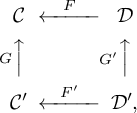
which is a natural isomorphism
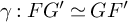 $\gamma : FG^{\prime } \simeq GF^{\prime }$
. If the functors
$\gamma : FG^{\prime } \simeq GF^{\prime }$
. If the functors
 $G^{\prime }, G$
have right adjoints
$G^{\prime }, G$
have right adjoints
 $H^{\prime }, H$
, then we have the natural transformation
$H^{\prime }, H$
, then we have the natural transformation
 $$\begin{align*}F^{\prime} H^{\prime} \xrightarrow{\mathrm{unit}} HG F^{\prime}H^{\prime} \stackrel{\gamma}{\simeq} HFG^{\prime}H^{\prime} \xrightarrow{\mathrm{counit}} HF, \end{align*}$$
called the associated exchange transformation. Similarly, if
 $G^{\prime }, G$
have left adjoints
$G^{\prime }, G$
have left adjoints
 $K^{\prime }, K$
, then we have the exchange transformation
$K^{\prime }, K$
, then we have the exchange transformation
 $$\begin{align*}KF \xrightarrow{\mathrm{unit}} KF G^{\prime}K^{\prime} \stackrel{\gamma}{\simeq} KGFK^{\prime} \xrightarrow{\mathrm{counit}} FK^{\prime}. \end{align*}$$
Suppose we have a commutative square of schemes

Then we have an induced commutative square of categories
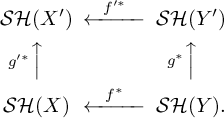
Passing to the right adjoints, we obtain the exchange transformation
 $$\begin{align*}\mathrm{Ex}^{*}_{*}: f^{*}g_{*} \to g^{\prime}_* f^{\prime*}. \end{align*}$$
Similarly, there is
 $\mathrm {Ex}_\#^*: g^{\prime }_\# f^{\prime *} \to f^*g_\#$
(for g smooth; this is in fact an equivalence if diagram (4) is cartesian), and so on.
$\mathrm {Ex}_\#^*: g^{\prime }_\# f^{\prime *} \to f^*g_\#$
(for g smooth; this is in fact an equivalence if diagram (4) is cartesian), and so on.
4.1.3 Exceptional exchange transformation
Given a cartesian square of schemes as in diagram (4), with g (and hence
 $g'$
) locally of finite type, there is a canonical equivalence
$g'$
) locally of finite type, there is a canonical equivalence
 $$\begin{align*}\mathrm{Ex}^*_!: f^*g_! \simeq g^{\prime}_! f^{\prime*}. \end{align*}$$
Passing to right adjoints, we obtain
 $$\begin{align*}\mathrm{Ex}^{*!}: f^{\prime*}g^! \to g^{\prime!}f^*. \end{align*}$$
4.1.4 Thom transformation
Given a perfect complex
 $\mathcal E$
of vector bundles on X, the motivic J-homomorphism
$\mathcal E$
of vector bundles on X, the motivic J-homomorphism
 $K(X) \to \mathrm {Pic}(\mathcal {SH}(X))$
[Reference Bachmann and Hoyois10, §16.2] provides us with an invertible spectrum
$K(X) \to \mathrm {Pic}(\mathcal {SH}(X))$
[Reference Bachmann and Hoyois10, §16.2] provides us with an invertible spectrum
![]() . We denote by
. We denote by
![]() the associated invertible endofunctor. If
the associated invertible endofunctor. If
 $\mathcal E$
is a vector bundle (concentrated in degree
$\mathcal E$
is a vector bundle (concentrated in degree
 $0$
), then
$0$
), then
![]() is the suspension spectrum on the Thom space
is the suspension spectrum on the Thom space
 $\mathcal E^*/\mathcal E^* \setminus 0$
.Footnote 6
$\mathcal E^*/\mathcal E^* \setminus 0$
.Footnote 6
Lemma 4.1. The functor
 $f^!$
commutes with Thom transforms.
$f^!$
commutes with Thom transforms.
Proof. This follows from the projection formula [Reference Cisinski and Déglise23, A.5.1(6)] and the invertibility of
:
4.1.5 Purity transformation
Let
 $f: X \to Y$
be a smoothable [Reference Elmanto, Hoyois, Khan, Sosnilo and Yakerson31, §2.1.21] lci morphism. Then the cotangent complex
$f: X \to Y$
be a smoothable [Reference Elmanto, Hoyois, Khan, Sosnilo and Yakerson31, §2.1.21] lci morphism. Then the cotangent complex
 $\mathrm {L}_f$
is perfect, and there exists a canonical purity transformation
$\mathrm {L}_f$
is perfect, and there exists a canonical purity transformation
 $$\begin{align*}\mathfrak{p}_f: \Sigma^{\mathrm{L}_f} f^* \to f^!. \end{align*}$$
4.2 Cohomology groups and Gysin maps
4.2.1
Let S be a scheme and set
 $E \in \mathcal {SH}(S)$
. Given
$E \in \mathcal {SH}(S)$
. Given
 $(\pi : X \to S) \in \mathrm {S}\mathrm {ch}{}_S$
,
$(\pi : X \to S) \in \mathrm {S}\mathrm {ch}{}_S$
,
 $i: Z \hookrightarrow X$
closed, and
$i: Z \hookrightarrow X$
closed, and
 $\xi \in K(Z)$
, we define the
$\xi \in K(Z)$
, we define the
 $\xi $
-twisted E-cohomology of X with support in Z as
$\xi $
-twisted E-cohomology of X with support in Z as
This assignment forms a cohomology theory in the sense of §3.1. It takes values in abelian groups, has supports, and satisfies the disjoint union property. We shall see that it has transfers for proper lci maps. It need not be orientable in general.
If
 $Z = X$
, we may omit it from the notation and just write
$Z = X$
, we may omit it from the notation and just write
 $E^\xi (X)$
. As before, if
$E^\xi (X)$
. As before, if
 $\xi $
is a trivial virtual vector bundle of rank
$\xi $
is a trivial virtual vector bundle of rank
 $n \in \mathbb {Z}$
, then we also write
$n \in \mathbb {Z}$
, then we also write
 $E^n_Z(X)$
instead of
$E^n_Z(X)$
instead of
 $E^\xi _Z(X)$
.
$E^\xi _Z(X)$
.
Example 4.2. Suppose that
 $\xi = i^*V$
, where V is a vector bundle on X. We have
$\xi = i^*V$
, where V is a vector bundle on X. We have
where we have used the fact that
 $i_* \simeq i_!$
and Lemma 4.1. Using the localization sequence
$i_* \simeq i_!$
and Lemma 4.1. Using the localization sequence
 $j_\#j^* \to \operatorname {id} \to i_*i^*$
[Reference Hoyois44, Theorem 6.18(4)] to identify
$j_\#j^* \to \operatorname {id} \to i_*i^*$
[Reference Hoyois44, Theorem 6.18(4)] to identify
, we find that
 $$\begin{align*}E_Z^\xi(X) \simeq \left[ X/(X \setminus Z), \Sigma^\xi \pi^* E\right]_{\mathcal{SH}(X)}. \end{align*}$$
Remark 4.3. The final expression in Example 4.2 depends only on
 $Z \subset X$
as a subset, not a subscheme. This also follows directly from the definition, since
$Z \subset X$
as a subset, not a subscheme. This also follows directly from the definition, since
 $\mathcal {SH}(Z) \simeq \mathcal {SH}(Z_{\mathrm {red}})$
; this is another consequence of localization.
$\mathcal {SH}(Z) \simeq \mathcal {SH}(Z_{\mathrm {red}})$
; this is another consequence of localization.
4.2.2 Functoriality in E
If
 $\alpha : E \to F \in \mathcal {SH}(S)$
is any morphism, then there is an induced morphism
$\alpha : E \to F \in \mathcal {SH}(S)$
is any morphism, then there is an induced morphism
 $\alpha _*: E^\xi _Z(X) \to F^\xi _Z(X)$
. This just follows from the fact that
$\alpha _*: E^\xi _Z(X) \to F^\xi _Z(X)$
. This just follows from the fact that
 $\pi ^*$
and so on are functors.
$\pi ^*$
and so on are functors.
4.2.3 Contravariant functoriality in X
Define
 $f: X^{\prime } \to X \in \mathrm {S}\mathrm {ch}{}_S$
. Then there is a pullback map
$f: X^{\prime } \to X \in \mathrm {S}\mathrm {ch}{}_S$
. Then there is a pullback map
 $$\begin{align*}f^*: E^\xi_Z(X) \to E^{f^* \xi}_{f^{-1}(Z)}(X^{\prime}), \end{align*}$$
coming from the morphism
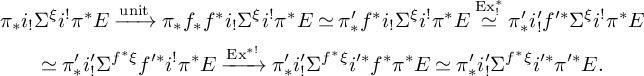 $$ \begin{gather*} \pi_* i_! \Sigma^\xi i^! \pi^* E \xrightarrow{\mathrm{unit}} \pi_* f_*f^* i_! \Sigma^\xi i^! \pi^* E \simeq \pi^{\prime}_* f^* i_! \Sigma^\xi i^! \pi^* E \stackrel{\mathrm{Ex}_!^*}{\simeq} \pi^{\prime}_* i^{\prime}_! f^{\prime*} \Sigma^\xi i^! \pi^* E \\ \simeq \pi^{\prime}_* i^{\prime}_! \Sigma^{f^*\xi} f^{\prime*} i^! \pi^* E \xrightarrow{\mathrm{Ex}^{*!}} \pi^{\prime}_* i^{\prime}_! \Sigma^{f^*\xi} i^{\prime*} f^* \pi^* E \simeq \pi^{\prime}_* i^{\prime}_! \Sigma^{f^*\xi} i^{\prime*} \pi^{\prime*} E. \end{gather*} $$
Here the
 $\mathrm {Ex}_!^*$
and
$\mathrm {Ex}_!^*$
and
 $\mathrm {Ex}^{*!}$
come from the cartesian square
$\mathrm {Ex}^{*!}$
come from the cartesian square
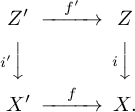
Lemma 4.4. Set
 $f: X^{\prime } \to X \in \mathrm {S}\mathrm {ch}{}_X$
,
$f: X^{\prime } \to X \in \mathrm {S}\mathrm {ch}{}_X$
,
 $Z \subset X$
,
$Z \subset X$
,
 $\xi \in K(Z)$
, and
$\xi \in K(Z)$
, and
 $\alpha : E \to F \in \mathcal {SH}(S)$
. The following square commutes:
$\alpha : E \to F \in \mathcal {SH}(S)$
. The following square commutes:
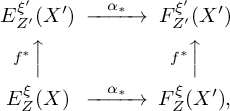
where
 $\xi ^{\prime } = f^*(\xi )$
and
$\xi ^{\prime } = f^*(\xi )$
and
 $Z^{\prime } = f^{-1}(Z)$
.
$Z^{\prime } = f^{-1}(Z)$
.
Proof. This is just an expression of the fact that the exchange transformations used to build
 $f^*$
are indeed natural transformations.
$f^*$
are indeed natural transformations.
4.2.4 Covariant functoriality in X
Suppose a commutative square in
 $\mathrm {S}\mathrm {ch}{}_S$
,
$\mathrm {S}\mathrm {ch}{}_S$
,

where f is smoothable lci,
 $i, k$
are closed immersions, and g is proper. For every
$i, k$
are closed immersions, and g is proper. For every
 $\xi \in K(Z_2)$
, there is a Gysin map
$\xi \in K(Z_2)$
, there is a Gysin map
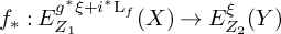 $$\begin{align*}f_*:E_{Z_1}^{g^* \xi + i^* \mathrm{L}_f}(X) \to E_{Z_2}^\xi(Y) \end{align*}$$
coming from the morphism
 $$\begin{align*}f_* i_! \Sigma^{g^*\xi + i^* \mathrm{L}_f} i^! f^* E_Y &\xrightarrow{\mathfrak{p}_f} f_* i_! \Sigma^{g^* \xi} i^! f^! E_Y \simeq k_! g_! \Sigma^{g^* \xi} g^!k^! E_Y \simeq k_! g_! g^!\Sigma^{\xi} k^! E_Y\\ &\xrightarrow{\mathrm{counit}} k_! \Sigma^\xi k^! E_Y, \end{align*}$$
where we used Lemma 4.1 to move
 $\Sigma ^{L_f}$
through
$\Sigma ^{L_f}$
through
 $i^!$
and
$i^!$
and
 $\Sigma ^\xi $
through
$\Sigma ^\xi $
through
 $g^!$
, and also used
$g^!$
, and also used
 $i_* \simeq i_!, k_* \simeq k_!, g_* \simeq g_!$
.
$i_* \simeq i_!, k_* \simeq k_!, g_* \simeq g_!$
.
Remark 4.5. In [Reference Elmanto, Hoyois, Khan, Sosnilo and Yakerson31], the Gysin map is denoted by
 $f_!$
, to emphasize that it involves the purity transform. We find the notation
$f_!$
, to emphasize that it involves the purity transform. We find the notation
 $f_*$
more convenient.
$f_*$
more convenient.
Lemma 4.6. The following hold:
-
(1) Suppose a square as in diagram (5) and
$\alpha : E \to F \in \mathcal {SH}(S)$
. Then the following square commutes: -
(2) Suppose a square as in diagram (5) and
$s: Y^{\prime } \to Y$
such that
$s, f$
are tor-independent. Set
$X^{\prime } = X \times _Y Y^{\prime }$
,
$Z_i^{\prime } = Z_i \times _Y Y^{\prime }$
,
$i^{\prime }, g^{\prime }, k^{\prime }, f^{\prime }$
the induced maps, and so on. Then the following square commutes: -
(3) Suppose a commutative diagram in
$\mathrm {S}\mathrm {ch}{}_S$
as followsThen given
$\xi \in K(Z_3)$
, we have Here we use the equivalence
$$\begin{align*}f^{\prime}_* f_* = (f^{\prime}f)_*: E^{\left(g^{\prime}g\right)^* \xi + i^* L_{f^{\prime}f}}_{Z_1}(X) \to E_{Z_3}^\xi(W). \end{align*}$$
$L_{f^{\prime }f} \simeq f^{\prime *} L_f + L_{f^{\prime }} \in K(X)$
, coming from the cofiber sequence
$f^{\prime *} L_f \to L_{f^{\prime }f} \to L_{f^{\prime }}$
.


Proof. (1) Since
 $f_*: E_{Z_1}^{g^* \xi + i^* \mathrm {L}_f}(X) \to E_{Z_2}^\xi (Y)$
is obtained as
$f_*: E_{Z_1}^{g^* \xi + i^* \mathrm {L}_f}(X) \to E_{Z_2}^\xi (Y)$
is obtained as
 $[1, \zeta _E]$
, where
$[1, \zeta _E]$
, where
 $\zeta $
is a natural transformation of endofunctors of
$\zeta $
is a natural transformation of endofunctors of
 $\mathcal {SH}(S)$
, this is clear.
$\mathcal {SH}(S)$
, this is clear.
(2) Consider the following diagram:
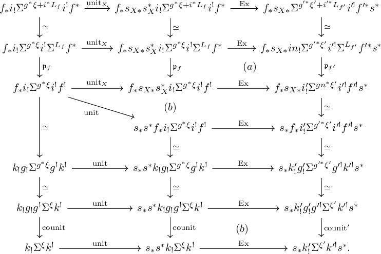
Here
 $s_X: X^{\prime } \to X$
is the canonical map and
$s_X: X^{\prime } \to X$
is the canonical map and
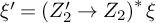 $\xi ^{\prime } = \left (Z_2^{\prime } \to Z_2\right )^* \xi $
. All the unlabeled equivalences arise from moving Thom transforms through (various) pullbacks, the compatibility of pullbacks and push-forwards with composition, and equivalences of the form
$\xi ^{\prime } = \left (Z_2^{\prime } \to Z_2\right )^* \xi $
. All the unlabeled equivalences arise from moving Thom transforms through (various) pullbacks, the compatibility of pullbacks and push-forwards with composition, and equivalences of the form
 $p_* \simeq p_!$
for p proper. All the maps labeled ‘
$p_* \simeq p_!$
for p proper. All the maps labeled ‘
 $\mathrm {Ex}$
’ are exchange transformations expressing the compatibility of
$\mathrm {Ex}$
’ are exchange transformations expressing the compatibility of
 $p_*, p_!, p^!$
with base change. Denote the diagram by
$p_*, p_!, p^!$
with base change. Denote the diagram by
 $\mathcal D$
. Then
$\mathcal D$
. Then
yields a diagram of abelian groups. The outer square of that diagram identifies with the square which we are trying to show commutes. It thus suffices to show that
 $\mathcal D$
commutes. All cells commute for trivial reasons, except for (a), which commutes by [Reference Elmanto, Hoyois, Khan, Sosnilo and Yakerson31, Proposition 2.2.2(ii)] and (b), which commute by the stability of the counit transformations under base change.
$\mathcal D$
commutes. All cells commute for trivial reasons, except for (a), which commutes by [Reference Elmanto, Hoyois, Khan, Sosnilo and Yakerson31, Proposition 2.2.2(ii)] and (b), which commute by the stability of the counit transformations under base change.
(3) Consider the following diagram:
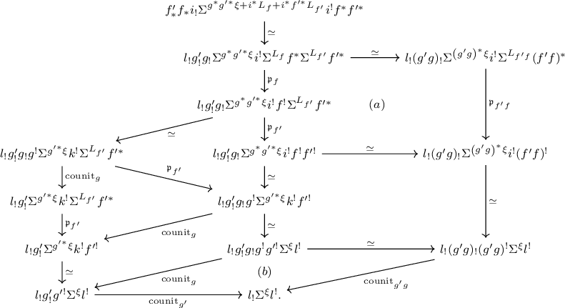
All the unlabeled equivalences arise from moving Thom transforms through (various) pullbacks, the compatibility of pullbacks and push-forwards with composition, and equivalences of the form
 $p_* \simeq p_!$
for p proper. Denote the diagram by
$p_* \simeq p_!$
for p proper. Denote the diagram by
 $\mathcal D$
. Then
$\mathcal D$
. Then
yields a diagram of abelian groups. Going from the top to the bottom middle via the leftmost path, we obtain
 $f^{\prime }_* f_*$
; going instead via the rightmost path we obtain
$f^{\prime }_* f_*$
; going instead via the rightmost path we obtain
 $(f^{\prime }f)_*$
. It hence suffices to show that
$(f^{\prime }f)_*$
. It hence suffices to show that
 $\mathcal D$
commutes. All cells commute for trivial reasons, except for (a), which commutes by [Reference Elmanto, Hoyois, Khan, Sosnilo and Yakerson31, Proposition 2.2.2(i)], and (b), which commutes by the compatibility of the counit transformations with composition.
$\mathcal D$
commutes. All cells commute for trivial reasons, except for (a), which commutes by [Reference Elmanto, Hoyois, Khan, Sosnilo and Yakerson31, Proposition 2.2.2(i)], and (b), which commutes by the compatibility of the counit transformations with composition.
Example 4.7. Consider a commutative square as in diagram (5), with
 $X=Y$
and
$X=Y$
and
 $f = \operatorname {id}$
, so that
$f = \operatorname {id}$
, so that
 $g: Z_1 \hookrightarrow Z_2$
is a closed immersion. Then
$g: Z_1 \hookrightarrow Z_2$
is a closed immersion. Then
 $f_*: E^{g^* \xi }_{Z_1}(X) \to E^\xi _{Z_2}(X)$
is the ‘extension of support’ map. In particular taking
$f_*: E^{g^* \xi }_{Z_1}(X) \to E^\xi _{Z_2}(X)$
is the ‘extension of support’ map. In particular taking
 $Z_2 = X$
as well, we obtain the map
$Z_2 = X$
as well, we obtain the map
 $E^{i^* \xi }_{Z_1}(X) \to E^\xi (X)$
‘forgetting the support’. Lemma 4.6(3) now in particular tells us that given a proper map
$E^{i^* \xi }_{Z_1}(X) \to E^\xi (X)$
‘forgetting the support’. Lemma 4.6(3) now in particular tells us that given a proper map
 $f: X \to Y$
, a closed immersion
$f: X \to Y$
, a closed immersion
 $i: Z \hookrightarrow X$
, and
$i: Z \hookrightarrow X$
, and
 $\xi \in K(Y)$
, the following diagram commutes:
$\xi \in K(Y)$
, the following diagram commutes:
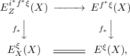
where the upper horizontal map forgets the support.
4.3 Orientations
4.3.1 Product structures
By a ring spectrum (over S) we an object
 $E \in \mathcal {SH}(S)$
together with homotopy classes of maps
$E \in \mathcal {SH}(S)$
together with homotopy classes of maps
![]() and
and
 $m: E \wedge E \to E$
satisfying the evident identities. If E is a ring spectrum, then there are multiplication maps
$m: E \wedge E \to E$
satisfying the evident identities. If E is a ring spectrum, then there are multiplication maps
 $$\begin{align*}E^\xi_{Z_1}(X) \times E^{\xi^{\prime}}_{Z_2}(X) \to E^{\xi + \xi^{\prime}}_{Z_1 \cap Z_2}(X) \end{align*}$$
induced by
 $$\begin{align*}\left(\Sigma^\xi E\right) \wedge \left(\Sigma^{\xi^{\prime}} E\right) \simeq \Sigma^{\xi + \xi^{\prime}} E \wedge E \xrightarrow{m} \Sigma^{\xi + \xi^{\prime}} E \end{align*}$$
and the diagonalFootnote 7
 $$\begin{align*}X/X \setminus (Z_1 \cap Z_2) \to X/X \setminus Z_1 \wedge X/X \setminus Z_2. \end{align*}$$
Lemma 4.8. The multiplicative structure on E-cohomology is compatible with pullback: given
 $Z_1, Z_2 \subset X$
,
$Z_1, Z_2 \subset X$
,
 $\xi , \xi ^{\prime } \in K(X)$
, and
$\xi , \xi ^{\prime } \in K(X)$
, and
 $f: X^{\prime } \to X$
, the following diagram commutes:
$f: X^{\prime } \to X$
, the following diagram commutes:
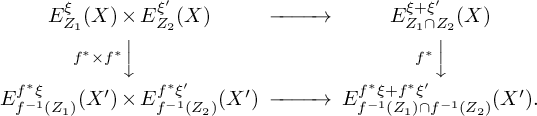
Proof. This is immediate from the definitions.
4.3.2 Thom spectra
Let
 $G = (G_n)_n$
be a family of finitely presented S-group schemes, equipped with a morphism of associative algebras
$G = (G_n)_n$
be a family of finitely presented S-group schemes, equipped with a morphism of associative algebras
 $G \to \left (\mathrm {GL}_{nk,S}\right )_n$
(for the Day convolution symmetric monoidal structure on
$G \to \left (\mathrm {GL}_{nk,S}\right )_n$
(for the Day convolution symmetric monoidal structure on
 $\mathrm {Fun}(\mathbb {N}, \mathrm {Grp}(\mathrm {S}\mathrm {ch}{}_S))$
). Then there is a notion of a (stable) vector bundle with structure group G, the associated K-theory space
$\mathrm {Fun}(\mathbb {N}, \mathrm {Grp}(\mathrm {S}\mathrm {ch}{}_S))$
). Then there is a notion of a (stable) vector bundle with structure group G, the associated K-theory space
 $K^G(X)$
, and the associated Thom spectrum
$K^G(X)$
, and the associated Thom spectrum
 $\mathrm {M} G$
, which is a ring spectrum [Reference Bachmann and Hoyois10, Example 16.22].
$\mathrm {M} G$
, which is a ring spectrum [Reference Bachmann and Hoyois10, Example 16.22].
Example 4.9. If
 $G_n = \mathrm {GL}_n$
, then
$G_n = \mathrm {GL}_n$
, then
 $K^G(X) = K(X)$
and
$K^G(X) = K(X)$
and
 $\mathrm {M} \mathrm {GL}$
is the algebraic cobordism spectrum [Reference Bachmann and Hoyois10, Theorem 16.13]. If
$\mathrm {M} \mathrm {GL}$
is the algebraic cobordism spectrum [Reference Bachmann and Hoyois10, Theorem 16.13]. If
 $G_n = \mathrm {SL}_n$
(resp.,
$G_n = \mathrm {SL}_n$
(resp.,
 $\mathrm {Sp}_n$
), then
$\mathrm {Sp}_n$
), then
 $K^G(X)$
is the K-theory of oriented (resp., symplectic) vector bundles in the usual sense, and
$K^G(X)$
is the K-theory of oriented (resp., symplectic) vector bundles in the usual sense, and
 $\mathrm {M} \mathrm {SL}$
(resp.,
$\mathrm {M} \mathrm {SL}$
(resp.,
 $\mathrm {M} \mathrm {Sp}$
) is the Thom spectrum as defined in [Reference Panin and Walter63].
$\mathrm {M} \mathrm {Sp}$
) is the Thom spectrum as defined in [Reference Panin and Walter63].
In order to work effectively with
 $\mathrm {M} G$
, one needs to know that it is stable under base change. This is easily seen to be true for
$\mathrm {M} G$
, one needs to know that it is stable under base change. This is easily seen to be true for
 $\mathrm {M}\mathrm {GL}$
,
$\mathrm {M}\mathrm {GL}$
,
 $\mathrm {M}\mathrm {SL}$
, and
$\mathrm {M}\mathrm {SL}$
, and
 $\mathrm {M}\mathrm {Sp}$
[Reference Bachmann and Hoyois10, Example 16.23]. We record the following more general result for future reference:
$\mathrm {M}\mathrm {Sp}$
[Reference Bachmann and Hoyois10, Example 16.23]. We record the following more general result for future reference:
Proposition 4.10. The Thom spectrum
 $\mathrm {M} G$
is stable under base change, provided that each
$\mathrm {M} G$
is stable under base change, provided that each
 $G_n$
is flat and quasi-affine.
$G_n$
is flat and quasi-affine.
Proof. We have a presheaf
 $K^G \in \mathcal {P}(\mathrm {S}\mathrm {ch}{}_S)$
and a map
$K^G \in \mathcal {P}(\mathrm {S}\mathrm {ch}{}_S)$
and a map
 $K^G \to K$
. For
$K^G \to K$
. For
 $f: X \to S \in \mathrm {S}\mathrm {ch}{}_S$
, denote by
$f: X \to S \in \mathrm {S}\mathrm {ch}{}_S$
, denote by
 $K^G_X \in \mathcal {P}({\mathrm {S}\mathrm {m}}_X)$
and
$K^G_X \in \mathcal {P}({\mathrm {S}\mathrm {m}}_X)$
and
 $j_X: K^G_X \to K\rvert _{{\mathrm {S}\mathrm {m}}_X}$
the restrictions. Then by definition,
$j_X: K^G_X \to K\rvert _{{\mathrm {S}\mathrm {m}}_X}$
the restrictions. Then by definition,
 $\mathrm {M} G_X = M_X(j_X)$
, where
$\mathrm {M} G_X = M_X(j_X)$
, where
 $M_X: \mathcal {P}({\mathrm {S}\mathrm {m}}_X)_{/K} \to \mathcal {SH}(X)$
is the motivic Thom-spectrum functor [Reference Bachmann and Hoyois10, §16.1]. Let
$M_X: \mathcal {P}({\mathrm {S}\mathrm {m}}_X)_{/K} \to \mathcal {SH}(X)$
is the motivic Thom-spectrum functor [Reference Bachmann and Hoyois10, §16.1]. Let
 $L K^G_S \in \mathcal {P}(\mathrm {S}\mathrm {ch}{}_S)$
denote the left Kan extension of
$L K^G_S \in \mathcal {P}(\mathrm {S}\mathrm {ch}{}_S)$
denote the left Kan extension of
 $K^G_S$
. We claim that
$K^G_S$
. We claim that
 $L K^G_S \to K^G$
is a Nisnevich equivalence. Assuming this, we deduce that
$L K^G_S \to K^G$
is a Nisnevich equivalence. Assuming this, we deduce that
 $f^* K^G_S \simeq \left .\left (L K^G_S\right )\right \rvert _{{\mathrm {S}\mathrm {m}}_X} \to K^G_X$
is a Nisnevich equivalence. Since
$f^* K^G_S \simeq \left .\left (L K^G_S\right )\right \rvert _{{\mathrm {S}\mathrm {m}}_X} \to K^G_X$
is a Nisnevich equivalence. Since
 $M_X$
inverts Nisnevich equivalences [Reference Bachmann and Hoyois10, Proposition 16.9], this implies that
$M_X$
inverts Nisnevich equivalences [Reference Bachmann and Hoyois10, Proposition 16.9], this implies that
 $f^* \mathrm {M} G_S \simeq \mathrm {M} G_X$
, which is the desired result.
$f^* \mathrm {M} G_S \simeq \mathrm {M} G_X$
, which is the desired result.
To prove the claim, we first note that by [Reference Elmanto, Hoyois, Khan, Sosnilo and Yakerson32, Lemma 3.3.9], we may assume S is affine, and it suffices to prove that the restriction of
 $K^G$
to
$K^G$
to
 ${\mathrm {A}\mathrm {ff}}_S$
is left Kan extended from smooth affine S-schemes. By definition,
${\mathrm {A}\mathrm {ff}}_S$
is left Kan extended from smooth affine S-schemes. By definition,
 $K^G = \left (\mathrm {Vect}^G\right )^{gp}$
, where
$K^G = \left (\mathrm {Vect}^G\right )^{gp}$
, where
 $\mathrm {Vect}^G = \coprod _{n \ge 0} BG_n$
(here the coproduct is as stacks i.e., fppf sheaves). The desired result now follows from [Reference Elmanto, Hoyois, Khan, Sosnilo and Yakerson32, Proposition A.0.4 and Lemma A.0.5] (noting that the coproduct of stacks is the same as the coproduct of
$\mathrm {Vect}^G = \coprod _{n \ge 0} BG_n$
(here the coproduct is as stacks i.e., fppf sheaves). The desired result now follows from [Reference Elmanto, Hoyois, Khan, Sosnilo and Yakerson32, Proposition A.0.4 and Lemma A.0.5] (noting that the coproduct of stacks is the same as the coproduct of
 $\Sigma $
-presheaves, and Kan extension preserves
$\Sigma $
-presheaves, and Kan extension preserves
 $\Sigma $
-presheaves).
$\Sigma $
-presheaves).
Now set
 $\xi \in K^G(X)$
. Then there is a canonical equivalence [Reference Bachmann and Hoyois10, Example 16.29]
$\xi \in K^G(X)$
. Then there is a canonical equivalence [Reference Bachmann and Hoyois10, Example 16.29]
 $$\begin{align*}\Sigma^\xi \mathrm{M} G_X \simeq \Sigma^{\lvert\xi\rvert} \mathrm{M} G_X. \end{align*}$$
We denote by
 $t_\xi \in \mathrm {M} G^{\xi - \lvert \xi \rvert }(X)$
the class of the map
$t_\xi \in \mathrm {M} G^{\xi - \lvert \xi \rvert }(X)$
the class of the map
4.3.3 Oriented ring spectra
Definition 4.11. Let
 $E \in \mathcal {SH}(S)$
be a ring spectrum and
$E \in \mathcal {SH}(S)$
be a ring spectrum and
 $G = (G_n)_n$
a family of group schemes as in §4.3.2. By a strong G -orientation of E we mean a ring map
$G = (G_n)_n$
a family of group schemes as in §4.3.2. By a strong G -orientation of E we mean a ring map
 $\mathrm {M} G \to E$
.
$\mathrm {M} G \to E$
.
Example 4.12. The spectrum
 $\mathrm {KO}$
is strongly
$\mathrm {KO}$
is strongly
 $\mathrm {SL}$
-oriented (see Corollary A.3).
$\mathrm {SL}$
-oriented (see Corollary A.3).
Note that if
 $E \in \mathcal {SH}(S)$
is strongly G-oriented, then there is no reason a priori why
$E \in \mathcal {SH}(S)$
is strongly G-oriented, then there is no reason a priori why
 $E_X$
should be strongly
$E_X$
should be strongly
 $G_X$
-oriented. This is true if
$G_X$
-oriented. This is true if
 $\mathrm {M} G$
is stable under base change, so for most reasonable G by Proposition 4.10. We will not talk about strong G-orientations unless
$\mathrm {M} G$
is stable under base change, so for most reasonable G by Proposition 4.10. We will not talk about strong G-orientations unless
 $\mathrm {M} G$
is stable under base change, so assume this throughout.
$\mathrm {M} G$
is stable under base change, so assume this throughout.
Given
 $\xi \in K^G(X)$
, the map
$\xi \in K^G(X)$
, the map
 $\mathrm {M} G \to E$
provides us with
$\mathrm {M} G \to E$
provides us with
 $t_\xi = t_\xi (E) \in E^{\xi - \lvert \xi \rvert }(X)$
.
$t_\xi = t_\xi (E) \in E^{\xi - \lvert \xi \rvert }(X)$
.
Proposition 4.13. Let E be strongly G-oriented and set
 $\xi \in K^G(X)$
.
$\xi \in K^G(X)$
.
-
(1) The classes
$t_\xi (E)$
are stable under base change: for
$f: X^{\prime } \to X$
we have
$t_{f^*\xi }(E) = f^*t_\xi (E)$
. -
(2) Multiplication by
$t_\xi (E)$
induces an equivalence
$\Sigma ^{\lvert \xi \rvert } E \simeq \Sigma ^\xi E$
and an isomorphism
$t: E^{\lvert \xi \rvert }_Z(X) \simeq E^\xi _Z(X)$
, called the Thom isomorphism. -
(3) The Thom isomorphism is compatible with base change:
$f^*(t(x)) = t(f^*(x))$
.


In particular, E is G-oriented.
Proof. (1) follows from the same statement for
 $\mathrm {M} G$
, where it holds by construction. For the first half of (2), it suffices to show that
$\mathrm {M} G$
, where it holds by construction. For the first half of (2), it suffices to show that
 $t_\xi (E)$
is a unit in the Picard-graded homotopy ring of E. This follows from the same statement for
$t_\xi (E)$
is a unit in the Picard-graded homotopy ring of E. This follows from the same statement for
 $\mathrm {M} G$
. The second half of (2) follows. (3) immediately follows from (1).
$\mathrm {M} G$
. The second half of (2) follows. (3) immediately follows from (1).
Example 4.14. Let E be strongly
 $\mathrm {GL}$
-oriented. Then for any
$\mathrm {GL}$
-oriented. Then for any
 $\xi \in K(X)$
we obtain
$\xi \in K(X)$
we obtain
 $E^\xi (X) \simeq E^{rk(\xi )}(X)$
, so E is oriented in the sense of §3.2.
$E^\xi (X) \simeq E^{rk(\xi )}(X)$
, so E is oriented in the sense of §3.2.
Definition 4.15. For
 $X \in \mathrm {S}\mathrm {ch}{}_S$
and
$X \in \mathrm {S}\mathrm {ch}{}_S$
and
 $\mathcal L$
a line bundle on X, put
$\mathcal L$
a line bundle on X, put
 $$\begin{align*}E^n_Z(X, \mathcal L) = E^{n-1+\mathcal L}_Z(X). \end{align*}$$
Example 4.16. Let E be strongly
 $\mathrm {SL}$
-oriented and set
$\mathrm {SL}$
-oriented and set
 $\xi \in K(X)$
. Then
$\xi \in K(X)$
. Then
 $\xi ^{\prime } := \xi - (\lvert \xi \rvert - 1 + \det \xi ) \in K(X)$
lifts canonically to
$\xi ^{\prime } := \xi - (\lvert \xi \rvert - 1 + \det \xi ) \in K(X)$
lifts canonically to
 $K^{\mathrm {SL}}(X)$
, whence by Proposition 4.13 we get a canonical (Thom) isomorphism
$K^{\mathrm {SL}}(X)$
, whence by Proposition 4.13 we get a canonical (Thom) isomorphism
 $E^\xi (X) \simeq E^{\lvert \xi \rvert }(X, \det \xi )$
. In particular, E is
$E^\xi (X) \simeq E^{\lvert \xi \rvert }(X, \det \xi )$
. In particular, E is
 $\mathrm {SL}$
-oriented in the sense of §3.2.
$\mathrm {SL}$
-oriented in the sense of §3.2.
Remark 4.17. If E is strongly
 $\mathrm {SL}$
-oriented, then since
$\mathrm {SL}$
-oriented, then since
 $\det (\mathcal L_1 \oplus \mathcal L_2) \simeq \mathcal L_1 \otimes \mathcal L_2$
, by Example 4.16 the product structure on E-cohomology twisted by line bundles takes the form
$\det (\mathcal L_1 \oplus \mathcal L_2) \simeq \mathcal L_1 \otimes \mathcal L_2$
, by Example 4.16 the product structure on E-cohomology twisted by line bundles takes the form
 $E^n(X, \mathcal L_1) \times E^m(X, \mathcal L_2) \to E^{n+m}(X, \mathcal L_1 \otimes \mathcal L_2)$
.
$E^n(X, \mathcal L_1) \times E^m(X, \mathcal L_2) \to E^{n+m}(X, \mathcal L_1 \otimes \mathcal L_2)$
.
Remark 4.18. Strong G-orientations have better permanence properties than ordinary ones (provided that
 $\mathrm {M} G$
is stable under base change): they are stable under base change and taking (very) effective covers, for example.
$\mathrm {M} G$
is stable under base change): they are stable under base change and taking (very) effective covers, for example.
4.4
$\mathrm {SL}^c$
-orientations

A. Ananyevskiy has done important work on
 $\mathrm {SL}$
and
$\mathrm {SL}$
and
 $\mathrm {SL}^c$
orientations. We shall make use of the following result (see, e.g., [Reference Ananyevskiy1, Theorem 1.1]):
$\mathrm {SL}^c$
orientations. We shall make use of the following result (see, e.g., [Reference Ananyevskiy1, Theorem 1.1]):
Proposition 4.19 Ananyevskiy
Let
 $E \in \mathcal {SH}(S)$
be
$E \in \mathcal {SH}(S)$
be
 $\mathrm {SL}$
-oriented and
$\mathrm {SL}$
-oriented and
 $\mathcal L_1, \mathcal L_2, \mathcal L_3$
be line bundles on X. Suppose an isomorphism
$\mathcal L_1, \mathcal L_2, \mathcal L_3$
be line bundles on X. Suppose an isomorphism
 $\mathcal L_1 \simeq \mathcal L_2 \otimes \mathcal L_3^{\otimes 2}$
.
$\mathcal L_1 \simeq \mathcal L_2 \otimes \mathcal L_3^{\otimes 2}$
.
-
(1) There is a canonical equivalence
$\Sigma ^{\mathcal L_1} E \simeq \Sigma ^{\mathcal L_2} E$
, compatible with base change. -
(2) There is a canonical isomorphism
$E^n_Z(X, \mathcal L_1) \simeq E^n_Z(X, \mathcal L_2)$
, compatible with base change.

In particular, the cohomology theory represented by E is
 $\mathrm {SL}^c$
-oriented.
$\mathrm {SL}^c$
-oriented.
Proof. Note that (2) follows from (1). Let
 $\mathcal L = \mathcal L_3$
. It suffices to exhibit a canonical equivalence
$\mathcal L = \mathcal L_3$
. It suffices to exhibit a canonical equivalence
 $\Sigma ^{\mathcal L^{\otimes 2}} E \simeq \Sigma ^{\mathcal O} E$
. We have canonical equivalences
$\Sigma ^{\mathcal L^{\otimes 2}} E \simeq \Sigma ^{\mathcal O} E$
. We have canonical equivalences
 $$\begin{align*}\Sigma^{\mathcal L + \mathcal L} E \simeq \Sigma^{\mathcal O + \mathcal L^{\otimes 2}} E, \qquad \Sigma^{\mathcal L + \mathcal L^*} E \simeq \Sigma^{\mathcal O^2}E, \qquad \Sigma^{\mathcal L + \mathcal L} \simeq \Sigma^{\mathcal L + \mathcal L^*}, \end{align*}$$
by [Reference Ananyevskiy1, Corollary 3.9, Lemma 4.1]. Consequently,
 $\Sigma ^{\mathcal O + \mathcal L^{\otimes 2}} E \simeq \Sigma ^{\mathcal O^2}E$
, whence the claim.
$\Sigma ^{\mathcal O + \mathcal L^{\otimes 2}} E \simeq \Sigma ^{\mathcal O^2}E$
, whence the claim.
5 Euler classes for representable theories
5.1 Tautological Euler class
Let
 $E \in \mathcal {SH}(S)$
be a ring spectrum, set
$E \in \mathcal {SH}(S)$
be a ring spectrum, set
 $X \in \mathrm {S}\mathrm {ch}{}_S$
, and let V be a vector bundle on X.
$X \in \mathrm {S}\mathrm {ch}{}_S$
, and let V be a vector bundle on X.
Definition 5.1. We denote by
 $e(V) = e(V, E) \in E^{V^*}(X)$
the tautological Euler class of V, defined as the composite
$e(V) = e(V, E) \in E^{V^*}(X)$
the tautological Euler class of V, defined as the composite
Lemma 5.2. Define
 $f: X^{\prime } \to X \in \mathrm {S}\mathrm {ch}{}_S$
. Then
$f: X^{\prime } \to X \in \mathrm {S}\mathrm {ch}{}_S$
. Then
 $$\begin{align*}f^* e(V, E) = e(f^*V, E) \in E^{f^* V}(X^{\prime}). \end{align*}$$
Proof. This is immediate.
If E is strongly
 $\mathrm {SL}$
-oriented in the sense of §4.3.3, and hence
$\mathrm {SL}$
-oriented in the sense of §4.3.3, and hence
 $\mathrm {SL}^c$
-oriented in the sense of §3.2, then for any relatively oriented vector bundle V over a smooth and proper scheme
$\mathrm {SL}^c$
-oriented in the sense of §3.2, then for any relatively oriented vector bundle V over a smooth and proper scheme
 $X/S$
we obtain an Euler number
$X/S$
we obtain an Euler number
 $n(V, \rho , E) \in E^0(S)$
(see §3.4).
$n(V, \rho , E) \in E^0(S)$
(see §3.4).
5.2 Integrally defined Euler numbers
Corollary 5.3 Euler numbers are stable under base change
Let E be a strongly
 $\mathrm {SL}$
-oriented cohomology theory and let V be vector bundle V over a smooth and proper scheme
$\mathrm {SL}$
-oriented cohomology theory and let V be vector bundle V over a smooth and proper scheme
 $X/S$
, relatively oriented by
$X/S$
, relatively oriented by
 $\rho $
. Let
$\rho $
. Let
 $f: S^{\prime } \to S$
be a morphism of schemes. Then
$f: S^{\prime } \to S$
be a morphism of schemes. Then
 $$\begin{align*}f^* n(V, \rho, E) = n(f^*V, f^*o, f^*E) \in E^0(S^{\prime}). \end{align*}$$
Proof. This holds because all our constructions are stable under base change–see in particular Lemma 4.6(2) (for the compatibility of Gysin maps with pullback, which applies since
 $X \to S$
is smooth), Propositions 4.19 and 4.13(3) (ensuring that the identification
$X \to S$
is smooth), Propositions 4.19 and 4.13(3) (ensuring that the identification
 $E^{V^*}(X) \simeq E^{L_\pi }(X)$
is compatible with base change), and Lemma 5.2 (for the compatibility of Euler classes with base change).
$E^{V^*}(X) \simeq E^{L_\pi }(X)$
is compatible with base change), and Lemma 5.2 (for the compatibility of Euler classes with base change).
Proposition 5.4. Let d be even or
 $d=1$
,
$d=1$
,
 $X/\mathbb {Z}[1/d]$
smooth and proper, and
$X/\mathbb {Z}[1/d]$
smooth and proper, and
 $V/X$
a relatively oriented vector bundle. Then for any field k with
$V/X$
a relatively oriented vector bundle. Then for any field k with
 $2d \in k^\times $
, we have
$2d \in k^\times $
, we have
 $$\begin{align*}n\left(V_k, \rho, \mathrm{H}\tilde{\mathbb{Z}}\right) \in \mathbb{Z}[\langle -1 \rangle, \langle 2 \rangle, \dots, \langle d \rangle] \subset \mathrm{GW}(k). \end{align*}$$
In fact, there is a formula
 $$\begin{align*}n\left(V_k, \rho, \mathrm{H}\tilde{\mathbb{Z}}\right) = \sum_{a \in \mathbb{Z}[1/d!]^\times} n_a \langle a \rangle, \end{align*}$$
which holds over any such field, with the coefficients
 $n_a \in \mathbb {Z}$
independent of k (and zero for all but finitely many a).
$n_a \in \mathbb {Z}$
independent of k (and zero for all but finitely many a).
Remark 5.5. If
 $d=1$
, Proposition 5.4 relies on the novel results about Hermitian K-theory of the integers from [Reference Calmès, Dotto, Harpaz, Hebestreit, Land, Moi, Nardin, Nikolaus and Steimle18]. In the following proof, this is manifested in the dependence of [Reference Bachmann and Hopkins9, Lemma 3.38(2)] on these results. We will later use Proposition 5.4 for the
$d=1$
, Proposition 5.4 relies on the novel results about Hermitian K-theory of the integers from [Reference Calmès, Dotto, Harpaz, Hebestreit, Land, Moi, Nardin, Nikolaus and Steimle18]. In the following proof, this is manifested in the dependence of [Reference Bachmann and Hopkins9, Lemma 3.38(2)] on these results. We will later use Proposition 5.4 for the
 $d=1$
case of Theorem 5.11, whence this result is also using [Reference Calmès, Dotto, Harpaz, Hebestreit, Land, Moi, Nardin, Nikolaus and Steimle18] in an essential way. For
$d=1$
case of Theorem 5.11, whence this result is also using [Reference Calmès, Dotto, Harpaz, Hebestreit, Land, Moi, Nardin, Nikolaus and Steimle18] in an essential way. For
 $d \geq 2$
, the proof is independent of [Reference Calmès, Dotto, Harpaz, Hebestreit, Land, Moi, Nardin, Nikolaus and Steimle18].
$d \geq 2$
, the proof is independent of [Reference Calmès, Dotto, Harpaz, Hebestreit, Land, Moi, Nardin, Nikolaus and Steimle18].
Note that here the assumption that the rank of V equals the dimension of X is included in the hypothesis that
 $V/X$
is a relatively oriented vector bundle (see Definition 1.5).
$V/X$
is a relatively oriented vector bundle (see Definition 1.5).
Proof. Recall the very effective cover functor
 $\tilde f_0$
and the truncation in the effective homotopy t-structure
$\tilde f_0$
and the truncation in the effective homotopy t-structure
 $\pi _0^{\mathrm {eff}}$
, for example from [Reference Bachmann5, §§3,4]. We have a diagram of spectra
$\pi _0^{\mathrm {eff}}$
, for example from [Reference Bachmann5, §§3,4]. We have a diagram of spectra
 $$\begin{align*}\mathrm{KO}_k \leftarrow \tilde f_0 \mathrm{KO}_k \to \pi_0^{\mathrm{eff}} \mathrm{KO}_k \leftarrow \pi_0^{\mathrm{eff}} \mathrm{MSL}_k \simeq H\tilde{\mathbb{Z}}; \end{align*}$$
see [Reference Bachmann and Hoyois10, Example 16.34] for the last equivalence. The functors
 $\tilde f_0$
and
$\tilde f_0$
and
 $\pi _0^{\mathrm {eff}}$
are lax monoidal in an appropriate sense, so this is a diagram of ring spectra. Moreover, all of the ring spectra are strongly
$\pi _0^{\mathrm {eff}}$
are lax monoidal in an appropriate sense, so this is a diagram of ring spectra. Moreover, all of the ring spectra are strongly
 $\mathrm {SL}$
-oriented (via the ring map
$\mathrm {SL}$
-oriented (via the ring map
 $\mathrm {MSL}_k \to \pi _0^{\mathrm {eff}} \mathrm {MSL}_k$
; see also Remark 4.18). Finally, all the maps induce isomorphisms on
$\mathrm {MSL}_k \to \pi _0^{\mathrm {eff}} \mathrm {MSL}_k$
; see also Remark 4.18). Finally, all the maps induce isomorphisms on
![]() , essentially by construction. It follows that
, essentially by construction. It follows that
 $n(V_k, \rho , \mathrm {KO}) = n\left (V_k, \rho , H\tilde {\mathbb {Z}}\right ) \in \mathrm {GW}(k)$
. We may thus just as well prove the result for
$n(V_k, \rho , \mathrm {KO}) = n\left (V_k, \rho , H\tilde {\mathbb {Z}}\right ) \in \mathrm {GW}(k)$
. We may thus just as well prove the result for
 $n(V_k, \rho , \mathrm {KO})$
instead.
$n(V_k, \rho , \mathrm {KO})$
instead.
If d is even, then we have
 $\mathrm {KO} \in \mathcal {SH}(\mathbb {Z}[1/d])$
, and by Corollary 5.3 we see that
$\mathrm {KO} \in \mathcal {SH}(\mathbb {Z}[1/d])$
, and by Corollary 5.3 we see that
 $n(V_k, \rho , \mathrm {KO}) \in im(\mathrm {GW}(\mathbb {Z}[1/d]) \to \mathrm {GW}(k))$
. The result thus follows from Lemma 5.6. If
$n(V_k, \rho , \mathrm {KO}) \in im(\mathrm {GW}(\mathbb {Z}[1/d]) \to \mathrm {GW}(k))$
. The result thus follows from Lemma 5.6. If
 $d=1$
, we use the
$d=1$
, we use the
 $\mathrm {SL}$
-oriented ring spectrum
$\mathrm {SL}$
-oriented ring spectrum
 $\mathrm {KO}^{\prime } \in \mathcal {SH}(\mathbb {Z})$
from [Reference Bachmann and Hopkins9, §3.8.3]. We find that
$\mathrm {KO}^{\prime } \in \mathcal {SH}(\mathbb {Z})$
from [Reference Bachmann and Hopkins9, §3.8.3]. We find that
 $n(V_k, \rho , \mathrm {KO})$
is the image of
$n(V_k, \rho , \mathrm {KO})$
is the image of
 $n(V, \rho , \mathrm {KO}^{\prime }) \in \mathrm {KO}^{\prime {^0}}(\mathbb {Z})$
. This latter group is isomorphic to
$n(V, \rho , \mathrm {KO}^{\prime }) \in \mathrm {KO}^{\prime {^0}}(\mathbb {Z})$
. This latter group is isomorphic to
 $\mathrm {GW}(\mathbb {Z})$
by [Reference Bachmann and Hopkins9, Lemma 3.38(2)], whence the result.
$\mathrm {GW}(\mathbb {Z})$
by [Reference Bachmann and Hopkins9, Lemma 3.38(2)], whence the result.
Lemma 5.6. Let d be even or
 $d=1$
. As a ring,
$d=1$
. As a ring,
 $\mathrm {GW}(\mathbb {Z}[1/d])$
is generated by
$\mathrm {GW}(\mathbb {Z}[1/d])$
is generated by
 $\langle -1 \rangle $
and
$\langle -1 \rangle $
and
 $\langle p \rangle $
, for the primes
$\langle p \rangle $
, for the primes
 $p \mid d$
.
$p \mid d$
.
Proof. Let
 $A = \mathbb {Z}[1/d]$
and
$A = \mathbb {Z}[1/d]$
and
 $U=\operatorname {Spec} A$
. If
$U=\operatorname {Spec} A$
. If
 $d=1$
, this is well known [Reference Milnor and Husemoller59, Theorem II.4.3]. Hence from now on,
$d=1$
, this is well known [Reference Milnor and Husemoller59, Theorem II.4.3]. Hence from now on,
 $1/2 \in A$
. Using Lemma B.2, it suffices to prove the analogous statement for
$1/2 \in A$
. Using Lemma B.2, it suffices to prove the analogous statement for
 $W(A)$
. Let
$W(A)$
. Let
 $I \subset W$
be the fundamental ideal and denote by
$I \subset W$
be the fundamental ideal and denote by
 $I^*$
its powers; we view these as presheaves on U. Consider the commutative graded ring
$I^*$
its powers; we view these as presheaves on U. Consider the commutative graded ring
 $k_* = H^*_{\mathrm {Nis}}\left (U, I^*/I^{*+1}\right )$
. Of course
$k_* = H^*_{\mathrm {Nis}}\left (U, I^*/I^{*+1}\right )$
. Of course
 $k_0 = \mathbb {Z}/2$
. It follows from [Reference Bachmann and Østvær11, Corollary 4.9], [Reference Bachmann7, Theorem 2.1, Lemma 2.7], and [Reference Spitzweck71, Theorem 3.9] that
$k_0 = \mathbb {Z}/2$
. It follows from [Reference Bachmann and Østvær11, Corollary 4.9], [Reference Bachmann7, Theorem 2.1, Lemma 2.7], and [Reference Spitzweck71, Theorem 3.9] that
 $k_1 \simeq \mathcal O^\times (U)/2$
and
$k_1 \simeq \mathcal O^\times (U)/2$
and
 $k_n \simeq \mathbb {Z}/2\{(-1)^n\}$
for
$k_n \simeq \mathbb {Z}/2\{(-1)^n\}$
for
 $n \ge 2$
. We have the classes
$n \ge 2$
. We have the classes
 $\langle a \rangle -1 \in I(U)$
(for
$\langle a \rangle -1 \in I(U)$
(for
 $a \in \mathcal O^\times (U)$
) showing that
$a \in \mathcal O^\times (U)$
) showing that
 $H^0_{\mathrm {Nis}}(U, I^n) \to k_n$
is surjective. The short exact sequences
$H^0_{\mathrm {Nis}}(U, I^n) \to k_n$
is surjective. The short exact sequences
 $$\begin{align*}0 \to H^0_{\mathrm{Nis}}\left(U, I^{n+1}\right) \to H^0_{\mathrm{Nis}}(U, I^{n}) \to k_n \end{align*}$$
thus show that
 $H^0_{\mathrm {Nis}}(U, W)$
is generated by the
$H^0_{\mathrm {Nis}}(U, W)$
is generated by the
 $\langle a \rangle $
together with
$\langle a \rangle $
together with
 $H^0_{\mathrm {Nis}}(U, I^n)$
, for any n. For n sufficiently large,
$H^0_{\mathrm {Nis}}(U, I^n)$
, for any n. For n sufficiently large,
 $H^0_{\mathrm {Nis}}(U, I^n) \simeq 2^nH^0_{ret}(U,\mathbb {Z}) \simeq 2^n\mathbb {Z}$
[Reference Bachmann7, Proposition 2.3] is generated by
$H^0_{\mathrm {Nis}}(U, I^n) \simeq 2^nH^0_{ret}(U,\mathbb {Z}) \simeq 2^n\mathbb {Z}$
[Reference Bachmann7, Proposition 2.3] is generated by
 $(\langle -1 \rangle -1)^n$
; thus
$(\langle -1 \rangle -1)^n$
; thus
 $H^0_{\mathrm {Nis}}(U, W)$
is generated by the
$H^0_{\mathrm {Nis}}(U, W)$
is generated by the
 $\langle a \rangle $
. It remains to observe that
$\langle a \rangle $
. It remains to observe that
 $H^0_{\mathrm {Nis}}(U, W) = W(U)$
. This follows from the descent spectral sequence for computing
$H^0_{\mathrm {Nis}}(U, W) = W(U)$
. This follows from the descent spectral sequence for computing
 $W(U) = [U, \mathrm {KW}]$
, using the fact that the motivic spectrum
$W(U) = [U, \mathrm {KW}]$
, using the fact that the motivic spectrum
 $\mathrm {KW}$
has
$\mathrm {KW}$
has
 $\underline \pi _* \mathrm {KW} = a_{\mathrm {Nis}} W$
for
$\underline \pi _* \mathrm {KW} = a_{\mathrm {Nis}} W$
for
 $* \equiv 0\ \,\pmod {4}$
and
$* \equiv 0\ \,\pmod {4}$
and
 $\underline \pi _* \mathrm {KW} = 0$
.
$\underline \pi _* \mathrm {KW} = 0$
.
Notation 5.7. Set
 $A \hookrightarrow \mathbb {R}$
and let V be a relatively oriented, rank n vector bundle on a smooth, proper n-dimensional scheme X over A. We have
$A \hookrightarrow \mathbb {R}$
and let V be a relatively oriented, rank n vector bundle on a smooth, proper n-dimensional scheme X over A. We have
 $\mathrm {GW}(\mathbb {R}) \simeq \mathbb {Z} \oplus \mathbb {Z}\langle -1 \rangle $
. There are thus unique integers
$\mathrm {GW}(\mathbb {R}) \simeq \mathbb {Z} \oplus \mathbb {Z}\langle -1 \rangle $
. There are thus unique integers
 $n_{\mathbb {R}}, n_{\mathbb {C}} \in \mathbb {Z}$
such that
$n_{\mathbb {R}}, n_{\mathbb {C}} \in \mathbb {Z}$
such that
 $$\begin{align*}n\left(V_{\mathbb{R}}, \rho, H\tilde{\mathbb{Z}}\right) = \frac{ n_{\mathbb{C}} + n_{\mathbb{R}} }{2} + \frac{n_{\mathbb{C}} - n_{\mathbb{R}}}{2}\langle -1 \rangle. \end{align*}$$
The integers
 $n_{\mathbb {R}}$
and
$n_{\mathbb {R}}$
and
 $n_{\mathbb {C}}$
are the Euler numbers of the corresponding real and complex topological vector bundles, respectively, at least when X is projective, justifying the notation. To show this, consider the cycle class map
$n_{\mathbb {C}}$
are the Euler numbers of the corresponding real and complex topological vector bundles, respectively, at least when X is projective, justifying the notation. To show this, consider the cycle class map
 $\mathrm {CH}^\ast (X) \to H^\ast (X(\mathbb {C}),\mathbb {Z})$
from the Chow ring of a smooth
$\mathrm {CH}^\ast (X) \to H^\ast (X(\mathbb {C}),\mathbb {Z})$
from the Chow ring of a smooth
 $\mathbb {C}$
-scheme X to the singular cohomology of the complex manifold
$\mathbb {C}$
-scheme X to the singular cohomology of the complex manifold
 $X(\mathbb {C})$
[Reference Fulton37, Chapter 19]. Furthermore, there are real cycle class maps from oriented Chow rings of
$X(\mathbb {C})$
[Reference Fulton37, Chapter 19]. Furthermore, there are real cycle class maps from oriented Chow rings of
 $\mathbb {R}$
-smooth schemes X to the singular cohomology of the real manifold
$\mathbb {R}$
-smooth schemes X to the singular cohomology of the real manifold
 $X(\mathbb {R})$
, discussed in [Reference Hornbostel, Wendt, Xie and Zibrowius43] (as well as more refined real cycle class maps defined in [Reference Benoist and Wittenberg13]): for a smooth
$X(\mathbb {R})$
, discussed in [Reference Hornbostel, Wendt, Xie and Zibrowius43] (as well as more refined real cycle class maps defined in [Reference Benoist and Wittenberg13]): for a smooth
 $\mathbb {R}$
-scheme X and a line bundle
$\mathbb {R}$
-scheme X and a line bundle
 $\mathcal {L} \to X$
, consider the real cycle class map
$\mathcal {L} \to X$
, consider the real cycle class map
 $$ \begin{align*}\widetilde{\mathrm{CH}}^\ast (X, \mathcal{L})\cong H^n\left(X, \mathrm{K}^{\mathrm{MW}}_n\left(\omega_{X/k}\right)\right) \cong H\tilde{\mathbb{Z}}^{L_{\pi}}(X) \to H^\ast(X(\mathbb{C}),\mathbb{Z}(\mathcal{L}))\end{align*} $$
from the oriented Chow groups twisted by
 $\mathcal {L}$
to the singular homology of the associated local system on
$\mathcal {L}$
to the singular homology of the associated local system on
 $X(\mathbb {R})$
. We use results on the real cycle class map due to Hornbostel, Wendt, Xie, and Zibrowius [Reference Hornbostel, Wendt, Xie and Zibrowius43], including compatibility with push-forwards. Since they only had need of this compatibility in the case of the push-forward by a closed immersion, we first extend it slightly:
$X(\mathbb {R})$
. We use results on the real cycle class map due to Hornbostel, Wendt, Xie, and Zibrowius [Reference Hornbostel, Wendt, Xie and Zibrowius43], including compatibility with push-forwards. Since they only had need of this compatibility in the case of the push-forward by a closed immersion, we first extend it slightly:
Lemma 5.8. Let
 $\pi : X \to \operatorname {Spec} k$
be the structure map of a smooth, projective scheme X of dimension n over the real numbers
$\pi : X \to \operatorname {Spec} k$
be the structure map of a smooth, projective scheme X of dimension n over the real numbers
 $\mathbb {R}$
. Then the following square commutes:
$\mathbb {R}$
. Then the following square commutes:
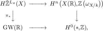
where the vertical maps are the canonical push-forwards and the horizontal maps are the real cycle class maps.
Proof. We have
 $\pi $
the composition of a closed immersion
$\pi $
the composition of a closed immersion
 $i: X \hookrightarrow \mathbb P^n_k$
and the structure map
$i: X \hookrightarrow \mathbb P^n_k$
and the structure map
 $p: \mathbb P^n_k \to \operatorname {Spec} k$
. The algebraic push-forward
$p: \mathbb P^n_k \to \operatorname {Spec} k$
. The algebraic push-forward
 $\pi _*$
is the composition
$\pi _*$
is the composition
 $p_* \circ i_*$
, and the analogous statement holds for the topological push-forward by classical algebraic topology. By [Reference Hornbostel, Wendt, Xie and Zibrowius43, Theorem 4.7], the push-forward
$p_* \circ i_*$
, and the analogous statement holds for the topological push-forward by classical algebraic topology. By [Reference Hornbostel, Wendt, Xie and Zibrowius43, Theorem 4.7], the push-forward
 $i_*$
commutes with real realization. We may thus reduce to the case where
$i_*$
commutes with real realization. We may thus reduce to the case where
 $X = \mathbb P^n_k$
is a projective n-space over a field k. In this case,
$X = \mathbb P^n_k$
is a projective n-space over a field k. In this case,
 $\pi _*$
is an isomorphism by [Reference Fasel33, Prop 6.3, Theorem 11.7]. Let
$\pi _*$
is an isomorphism by [Reference Fasel33, Prop 6.3, Theorem 11.7]. Let
 $s : \operatorname {Spec} K \to \mathbb P^n_k$
be the closed immersion given by the origin. Since
$s : \operatorname {Spec} K \to \mathbb P^n_k$
be the closed immersion given by the origin. Since
 $\pi s = 1$
, and the real realization maps commute with the algebraic and topological push-forwards of s by [Reference Hornbostel, Wendt, Xie and Zibrowius43, Theorem 4.7], the real realization maps also commute with the algebraic and topological push-forwards of
$\pi s = 1$
, and the real realization maps commute with the algebraic and topological push-forwards of s by [Reference Hornbostel, Wendt, Xie and Zibrowius43, Theorem 4.7], the real realization maps also commute with the algebraic and topological push-forwards of
 $\pi $
.
$\pi $
.
Proposition 5.9. Set
 $A \hookrightarrow \mathbb {R}$
and let V be a relatively oriented, rank n vector bundle on a smooth projective n-dimensional scheme X over A. Then
$A \hookrightarrow \mathbb {R}$
and let V be a relatively oriented, rank n vector bundle on a smooth projective n-dimensional scheme X over A. Then
 $n_{\mathbb {R}}$
and
$n_{\mathbb {R}}$
and
 $n_{\mathbb {C}}$
are the Euler numbers of the corresponding real and complex topological vector bundles, respectively–that is,
$n_{\mathbb {C}}$
are the Euler numbers of the corresponding real and complex topological vector bundles, respectively–that is,
 $n_{\mathbb {R}}$
is the topological Euler number of the relatively oriented topological
$n_{\mathbb {R}}$
is the topological Euler number of the relatively oriented topological
 $\mathbb {R}^n$
-bundle
$\mathbb {R}^n$
-bundle
 $V(\mathbb {R})$
associated to the real points of V on the real n-manifold
$V(\mathbb {R})$
associated to the real points of V on the real n-manifold
 $X(\mathbb {R})$
, and
$X(\mathbb {R})$
, and
 $n_{\mathbb {C}}$
is the analogous topological Euler number on
$n_{\mathbb {C}}$
is the analogous topological Euler number on
 $V(\mathbb {C}) \to X(\mathbb {C})$
.
$V(\mathbb {C}) \to X(\mathbb {C})$
.
Proof. By [Reference Hornbostel, Wendt, Xie and Zibrowius43, Proposition 6.1], the
 $\mathbb A^1$
-Euler class
$\mathbb A^1$
-Euler class
 $e\left (V, H\tilde {\mathbb {Z}}\right )$
of
$e\left (V, H\tilde {\mathbb {Z}}\right )$
of
 $V_{\mathbb {R}}$
in the oriented Chow group
$V_{\mathbb {R}}$
in the oriented Chow group
 $H\tilde {\mathbb {Z}}^{V^*}(X_{\mathbb {R}}) $
maps to the topological Euler class of
$H\tilde {\mathbb {Z}}^{V^*}(X_{\mathbb {R}}) $
maps to the topological Euler class of
 $V(\mathbb {R})$
under the real cycle class map. By Lemma 5.8, it follows that the image of the Euler number
$V(\mathbb {R})$
under the real cycle class map. By Lemma 5.8, it follows that the image of the Euler number
 $n\left (V,H\tilde {\mathbb {Z}}\right )$
under the real cycle class map is the topological Euler number of
$n\left (V,H\tilde {\mathbb {Z}}\right )$
under the real cycle class map is the topological Euler number of
 $V(\mathbb {R})$
. Under the canonical isomorphism
$V(\mathbb {R})$
. Under the canonical isomorphism
 $H^0(\ast , \mathbb {Z}) \cong \mathbb {Z}$
, the real cycle class map
$H^0(\ast , \mathbb {Z}) \cong \mathbb {Z}$
, the real cycle class map
 $\mathrm {GW}(\mathbb {R}) \to H^0(\ast , \mathbb {Z}) \cong \mathbb {Z}$
is the map taking a bilinear form over
$\mathrm {GW}(\mathbb {R}) \to H^0(\ast , \mathbb {Z}) \cong \mathbb {Z}$
is the map taking a bilinear form over
 $\mathbb {R}$
to its signature. It follows that
$\mathbb {R}$
to its signature. It follows that
 $n_{\mathbb {R}}$
is the topological Euler number of
$n_{\mathbb {R}}$
is the topological Euler number of
 $V(\mathbb {R})$
.
$V(\mathbb {R})$
.
Let
 $\gamma : \widetilde {\mathrm {CH}}^\ast (X, \det V^*) \cong H\tilde {\mathbb {Z}}^{V^*}(X_{\mathbb {R}}) \to \mathrm {CH}^{\ast }(X) \to \mathrm {CH}^{\ast }(X_{\mathbb {C}}) \to H^{\ast }(X(\mathbb {C}), \mathbb {Z})$
denote the composition of the canonical map to Chow followed by the (usual) cycle class map, and we similarly have
$\gamma : \widetilde {\mathrm {CH}}^\ast (X, \det V^*) \cong H\tilde {\mathbb {Z}}^{V^*}(X_{\mathbb {R}}) \to \mathrm {CH}^{\ast }(X) \to \mathrm {CH}^{\ast }(X_{\mathbb {C}}) \to H^{\ast }(X(\mathbb {C}), \mathbb {Z})$
denote the composition of the canonical map to Chow followed by the (usual) cycle class map, and we similarly have
 $$ \begin{align*}\gamma: \mathrm{GW}(\mathbb{R}) \cong \widetilde{\mathrm{CH}}^{0}(\operatorname{Spec} \mathbb{R}) \to H^{0}(\operatorname{Spec} \mathbb{R} (\mathbb{C}), \mathbb{Z}) \cong H^0(\ast, \mathbb{Z}) \cong \mathbb{Z},\end{align*} $$
which sends the class of a bilinear form in
 $\mathrm {GW}(\mathbb {R})$
to its rank. The cycle class map is compatible with Chern classes ([Reference Fulton37, Proposition 19.1.2]), whence the image of
$\mathrm {GW}(\mathbb {R})$
to its rank. The cycle class map is compatible with Chern classes ([Reference Fulton37, Proposition 19.1.2]), whence the image of
 $e\left (V, H\tilde {\mathbb {Z}}\right )$
under
$e\left (V, H\tilde {\mathbb {Z}}\right )$
under
 $\gamma $
is the topological Euler class of
$\gamma $
is the topological Euler class of
 $V(\mathbb {C})$
. The cycle class map commutes with the relevant push-forwards and pullbacks [Reference Fulton37, Corollary 19.2, Example 19.2.1], so we have that
$V(\mathbb {C})$
. The cycle class map commutes with the relevant push-forwards and pullbacks [Reference Fulton37, Corollary 19.2, Example 19.2.1], so we have that
 $\gamma \left (n\left (V,H\tilde {\mathbb {Z}}\right )\right ) = n_{\mathbb {C}}$
is the topological Euler number of
$\gamma \left (n\left (V,H\tilde {\mathbb {Z}}\right )\right ) = n_{\mathbb {C}}$
is the topological Euler number of
 $V(\mathbb {C})$
.
$V(\mathbb {C})$
.
Remark 5.10. If proper push-forwards in algebra and topology commute with real realization, as predicted by [Reference Hornbostel, Wendt, Xie and Zibrowius43, 4.5 Remark], then Proposition 5.9 holds more generally for smooth, proper schemes. It seems that proving this would take us too far afield, however. Alternatively, if
 $V \otimes \mathbb {R}$
admits a nondegenerate section, then the results of §8 (showing that the Euler number can be computed in terms of Scheja–Storch forms) imply that Proposition 5.9 holds for smooth, proper schemes, arguing as in [Reference Srinivasan and Wickelgren72, Lemma 5].
$V \otimes \mathbb {R}$
admits a nondegenerate section, then the results of §8 (showing that the Euler number can be computed in terms of Scheja–Storch forms) imply that Proposition 5.9 holds for smooth, proper schemes, arguing as in [Reference Srinivasan and Wickelgren72, Lemma 5].
Theorem 5.11. Suppose X is smooth and proper over
 $\mathbb {Z}[1/2]$
. Let V be a relatively oriented vector bundle on X and let
$\mathbb {Z}[1/2]$
. Let V be a relatively oriented vector bundle on X and let
 $V_k$
denote the base change of V to k for any field k. Then one of the following is true:
$V_k$
denote the base change of V to k for any field k. Then one of the following is true:
 $$ \begin{align} n^{\mathrm{GS}}(V_k, \rho) = \frac{ n_{\mathbb{C}} +n_{\mathbb{R}} }{2} + \frac{n_{\mathbb{C}} - n_{\mathbb{R}}}{2}\langle -1 \rangle\end{align} $$
or
 $$ \begin{align} n^{\mathrm{GS}}(V_k, \rho) = \frac{ n_{\mathbb{C}} +n_{\mathbb{R}} }{2} + \frac{n_{\mathbb{C}} - n_{\mathbb{R}}}{2}\langle -1 \rangle + \langle 2 \rangle -1,\end{align} $$
where the same formula holds for all fields k of characteristic
 $\ne 2$
.
$\ne 2$
.
If instead X is smooth and proper over
 $\mathbb {Z}$
, then equation (6) holds for any field k (including fields k of characteristic
$\mathbb {Z}$
, then equation (6) holds for any field k (including fields k of characteristic
 $2$
).
$2$
).
Recall that for the last claim regarding X smooth and proper over
 $\mathbb {Z}$
, we rely on [Reference Calmès, Dotto, Harpaz, Hebestreit, Land, Moi, Nardin, Nikolaus and Steimle18] (see Remark 5.5).
$\mathbb {Z}$
, we rely on [Reference Calmès, Dotto, Harpaz, Hebestreit, Land, Moi, Nardin, Nikolaus and Steimle18] (see Remark 5.5).
Proof. First assume that
 $char(k) \ne 2$
. By Corollary 1.4, we have
$char(k) \ne 2$
. By Corollary 1.4, we have
 $n^{\mathrm {GS}}(V_k, \rho ) = n\left (V_k, \rho , H\tilde {\mathbb {Z}}\right )$
. If the base is
$n^{\mathrm {GS}}(V_k, \rho ) = n\left (V_k, \rho , H\tilde {\mathbb {Z}}\right )$
. If the base is
 $\mathbb {Z}$
, then we learn from Proposition 5.4 that there exist
$\mathbb {Z}$
, then we learn from Proposition 5.4 that there exist
 $a, b \in \mathbb {Z}$
(independent of k!) such that
$a, b \in \mathbb {Z}$
(independent of k!) such that
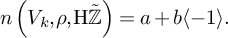 $$\begin{align*}n\left(V_k, \rho, \mathrm{H}\tilde{\mathbb{Z}}\right) = a + b\langle -1 \rangle. \end{align*}$$
In
 $\mathrm {GW}(\mathbb {Z}[1/2]) \hookrightarrow \mathrm {GW}(\mathbb {Q})$
we have the relations
$\mathrm {GW}(\mathbb {Z}[1/2]) \hookrightarrow \mathrm {GW}(\mathbb {Q})$
we have the relations
 $$\begin{align*}\langle -2 \rangle = 1 + \langle -1 \rangle - \langle 2 \rangle \quad \text{and} \quad 2\langle 2 \rangle = 2 \end{align*}$$
(the former because
 $\langle a \rangle + \langle -a \rangle = \langle 1 \rangle + \langle -1 \rangle $
for any a, and see, e.g., [Reference Bachmann6, Lemma 42] for the latter). Hence if the base is
$\langle a \rangle + \langle -a \rangle = \langle 1 \rangle + \langle -1 \rangle $
for any a, and see, e.g., [Reference Bachmann6, Lemma 42] for the latter). Hence if the base is
 $\mathbb {Z}[1/2]$
, there exist
$\mathbb {Z}[1/2]$
, there exist
 $a, b \in \mathbb {Z}, c \in \{0,1\}$
(independent of the choice of field k!) such that
$a, b \in \mathbb {Z}, c \in \{0,1\}$
(independent of the choice of field k!) such that
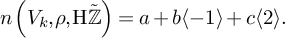 $$\begin{align*}n\left(V_k, \rho, \mathrm{H}\tilde{\mathbb{Z}}\right) = a + b\langle -1 \rangle + c \langle 2 \rangle. \end{align*}$$
If the base is
 $\mathbb {Z}$
, let us put
$\mathbb {Z}$
, let us put
 $c=0$
. By construction we have
$c=0$
. By construction we have
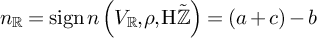 $$ \begin{align*}n_{\mathbb{R}} = \operatorname{sign} n\left(V_{\mathbb{R}}, \rho, \mathrm{H}\tilde{\mathbb{Z}}\right)=(a+c)-b\end{align*} $$
and
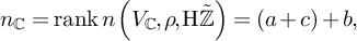 $$ \begin{align*}n_{\mathbb{C}} = \operatorname{rank} n\left(V_{\mathbb{C}}, \rho, \mathrm{H}\tilde{\mathbb{Z}}\right)=(a+c)+b,\end{align*} $$
which determines
 $a+c$
and b, so that there remain only at most two possible values for
$a+c$
and b, so that there remain only at most two possible values for
 $n\left (V_k,\rho ,\mathrm {H}\tilde {\mathbb {Z}}\right )$
.
$n\left (V_k,\rho ,\mathrm {H}\tilde {\mathbb {Z}}\right )$
.
Now suppose that
 $char(k) = 2$
(so that in particular the base is
$char(k) = 2$
(so that in particular the base is
 $\mathbb {Z}$
). Since
$\mathbb {Z}$
). Since
 $\langle 1 \rangle = \langle -1 \rangle $
over fields of characteristic
$\langle 1 \rangle = \langle -1 \rangle $
over fields of characteristic
 $2$
, we need to show that
$2$
, we need to show that
 $n^{\mathrm {GS}}(V_k, \rho ) = n_{\mathbb {C}}$
. We may as well assume that
$n^{\mathrm {GS}}(V_k, \rho ) = n_{\mathbb {C}}$
. We may as well assume that
 $k=\mathbb {F}_2$
. The rank induces an isomorphism
$k=\mathbb {F}_2$
. The rank induces an isomorphism
 $\mathrm {GW}(\mathbb {F}_2) \cong \mathbb {Z}$
(see, e.g., Corollary B.4). Considering the canonical maps
$\mathrm {GW}(\mathbb {F}_2) \cong \mathbb {Z}$
(see, e.g., Corollary B.4). Considering the canonical maps
 $$\begin{align*}\mathrm{GW}(\mathbb{F}_2) \to \mathrm{KGL}^0(\mathbb{F}_2) \leftarrow \mathrm{KGL}^0(\mathbb{Z}) \to \mathrm{KGL}^0(\mathbb{Z}[1/2]) \leftarrow \mathrm{GW}(\mathbb{Z}[1/2]), \end{align*}$$
in which all but the right-most one are isomorphisms, we get the string of equalities
 $$\begin{align*}n\left(V_{\mathbb{F}_2}\right) = n\left(V_{\mathbb{F}_2}, \mathrm{KGL}\right) = n(V_{\mathbb{Z}}, \mathrm{KGL}) = n\left(V_{\mathbb{Z}\left[1/2\right]}, \mathrm{KGL}\right) = rk\left(n\left(V_{\mathbb{Z}\left[1/2\right]}, \mathrm{KO}\right)\right). \end{align*}$$
The result follows.
Remark 5.12. The difference of the two values given in Theorem 5.11 is
 $\langle 2 \rangle - 1$
, so the two possibilities can be distinguished by the value of
$\langle 2 \rangle - 1$
, so the two possibilities can be distinguished by the value of
 $\operatorname {disc} n(V_k)$
in
$\operatorname {disc} n(V_k)$
in
 $k^*/(k^*)^2$
for any field k in which
$k^*/(k^*)^2$
for any field k in which
 $2$
is not a square, such as
$2$
is not a square, such as
 $\mathbb {F}_3$
or
$\mathbb {F}_3$
or
 $\mathbb {F}_5$
. Such discriminants can be evaluated by a computer, as shown to the second author by Anton Leyton and Sabrina Pauli.
$\mathbb {F}_5$
. Such discriminants can be evaluated by a computer, as shown to the second author by Anton Leyton and Sabrina Pauli.
5.3 Refined Euler classes and numbers
Definition 5.13 refined Euler class
Let
 $E \in \mathcal {SH}(S)$
be a homotopy ring spectrum, set
$E \in \mathcal {SH}(S)$
be a homotopy ring spectrum, set
 $X \in \mathrm {S}\mathrm {ch}{}_S$
, and let
$X \in \mathrm {S}\mathrm {ch}{}_S$
, and let
 $V \to X$
be a vector bundle and
$V \to X$
be a vector bundle and
 $\sigma : X \to V$
a section with zero scheme
$\sigma : X \to V$
a section with zero scheme
 $Z = Z(\sigma )$
. We denote by
$Z = Z(\sigma )$
. We denote by
 $e(V, \sigma ) = e(V, \sigma , E) \in E^{V^*}_Z(X)$
the class corresponding to the composite
$e(V, \sigma ) = e(V, \sigma , E) \in E^{V^*}_Z(X)$
the class corresponding to the composite
(see Example 4.2).
Remark 5.14. It is clear by construction that refined Euler classes are stable under base change.
Remark 5.15. In [Reference Levine and Raksit56, Definition 3.9] the authors define for an
 $\mathrm {SL}$
-oriented ring spectrum E and a vector bundle
$\mathrm {SL}$
-oriented ring spectrum E and a vector bundle
 $p: V \to X$
the canonical Thom class
$p: V \to X$
the canonical Thom class
 $th(V) \in E^{p^*V}_0(V)$
, which one can check coincides with
$th(V) \in E^{p^*V}_0(V)$
, which one can check coincides with
 $e(p^*V, \sigma _0)$
, where
$e(p^*V, \sigma _0)$
, where
 $\sigma _0$
is the tautological section of
$\sigma _0$
is the tautological section of
 $p^*V$
. Since
$p^*V$
. Since
 $e(V, \sigma ) = \sigma ^* e(p^*V, \sigma _0)$
, we deduce that
$e(V, \sigma ) = \sigma ^* e(p^*V, \sigma _0)$
, we deduce that
 $$\begin{align*}e(V, \sigma) = \sigma^* th(V). \end{align*}$$
Lemma 5.16. The ‘forgetting support’ map
 $E_Z^{V^*}(X) \to E^{V^*}(X)$
sends
$E_Z^{V^*}(X) \to E^{V^*}(X)$
sends
 $e(V, \sigma )$
to
$e(V, \sigma )$
to
 $e(V)$
.
$e(V)$
.
Proof. This follows from the commutative diagram
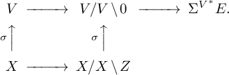
Indeed the composite from the bottom left to the top right along the top left represents
 $e(V)$
, by Definition 5.1 (note that
$e(V)$
, by Definition 5.1 (note that
 $\sigma $
is a homotopy inverse to the projection
$\sigma $
is a homotopy inverse to the projection
 $V \to X$
), whereas the composite along the bottom right represents
$V \to X$
), whereas the composite along the bottom right represents
 $e(V, \sigma )$
with support forgotten, by Definition 5.13 and Example 4.2.
$e(V, \sigma )$
with support forgotten, by Definition 5.13 and Example 4.2.
Definition 5.17 refined Euler number
Suppose that
 $\pi : X \to S$
is smoothable lci,
$\pi : X \to S$
is smoothable lci,
 $Z \to S$
is finite, and V is relatively oriented (so in particular,
$Z \to S$
is finite, and V is relatively oriented (so in particular,
 $rk(V) = rk(\mathrm {L}_\pi )$
). Suppose further that E is
$rk(V) = rk(\mathrm {L}_\pi )$
). Suppose further that E is
 $\mathrm {SL}$
-oriented. Then we put
$\mathrm {SL}$
-oriented. Then we put
 $$\begin{align*}n(V, \sigma, \rho) = n(V, \sigma, \rho, E) = \pi_* e(V, \sigma) \in E^0(S). \end{align*}$$
Corollary 5.18. Suppose that additionally
 $\pi : X \to S$
is smooth and proper. Then
$\pi : X \to S$
is smooth and proper. Then
 $n(V, \sigma , \rho ) = n(V, \rho ) \in E^0(S)$
.
$n(V, \sigma , \rho ) = n(V, \rho ) \in E^0(S)$
.
5.4 Refined Euler classes and the six-functors formalism
We now relate our Euler classes to the six-functors formalism. The following result shows that our refined Euler class coincides with the one defined by Déglise, Jin, and Khan [Reference Déglise, Jin and Khan26, Remark 3.2.10]:
Proposition 5.19. Let
 $E \in \mathcal {SH}(S)$
be a homotopy ring spectrum, set
$E \in \mathcal {SH}(S)$
be a homotopy ring spectrum, set
 $X \in {\mathrm {S}\mathrm {m}}_S$
, and let V be a vector bundle over X and
$X \in {\mathrm {S}\mathrm {m}}_S$
, and let V be a vector bundle over X and
 $\sigma $
a section of V. Then
$\sigma $
a section of V. Then
 $$\begin{align*}e(V, \sigma, E) = \sigma^*z_*(1), \end{align*}$$
where
 $z: X \to V$
is the zero section and we use the canonical isomorphism
$z: X \to V$
is the zero section and we use the canonical isomorphism
 $N_z \simeq V$
to form the push-forward
$N_z \simeq V$
to form the push-forward
 $z_*$
.
$z_*$
.
Proof. Let
 $p: V \to X$
be the projection and
$p: V \to X$
be the projection and
 $s_0: V \to p^* V$
the canonical section. Then
$s_0: V \to p^* V$
the canonical section. Then
 $\sigma ^*(p^*V, \sigma _0) = (V, s)$
, and hence, using Remark 5.14, it suffices to show that
$\sigma ^*(p^*V, \sigma _0) = (V, s)$
, and hence, using Remark 5.14, it suffices to show that
 $z_*(1) = e(p^*V, \sigma _0, E)$
. By [Reference Elmanto, Hoyois, Khan, Sosnilo and Yakerson31, last sentence of §2.1.1], we know that
$z_*(1) = e(p^*V, \sigma _0, E)$
. By [Reference Elmanto, Hoyois, Khan, Sosnilo and Yakerson31, last sentence of §2.1.1], we know that
 $$\begin{align*}z_*: E^0(X) \simeq E^{z^* p^*V^* + L_z} \to E^{p^*V^*}_X(V) \end{align*}$$
is the purity equivalence. In the case of the zero section of a vector bundle, it just takes the tautological form
and hence indeed sends
 $1$
to
$1$
to
 $e(p^*V, \sigma _0)$
.
$e(p^*V, \sigma _0)$
.
It follows from the foregoing that Euler classes of vector bundles are determined by Euler classes of vector bundles with nondegenerate sections.
Example 5.20. Let
 $V \to X$
be a vector bundle and
$V \to X$
be a vector bundle and
 $\sigma $
a section. Suppose
$\sigma $
a section. Suppose
 $1/2 \in S$
. The Euler class of V in
$1/2 \in S$
. The Euler class of V in
 $\mathrm {KW} = \mathrm {KO}\left [\eta ^{-1}\right ]$
is given by the Koszul complex with its canonical symmetric bilinear form. Indeed, we may assume that V has a regular section, in which case this follows from the existence of the morphism of cohomology theories
$\mathrm {KW} = \mathrm {KO}\left [\eta ^{-1}\right ]$
is given by the Koszul complex with its canonical symmetric bilinear form. Indeed, we may assume that V has a regular section, in which case this follows from the existence of the morphism of cohomology theories
 $\mathrm {BL}^{\mathrm {naive}} \to \mathrm {KW}$
and Proposition 2.11.
$\mathrm {BL}^{\mathrm {naive}} \to \mathrm {KW}$
and Proposition 2.11.
We deduce that Meta-Theorem 3.9 holds in this setting, even in a slightly stronger form with supports:
Corollary 5.21. If
 $\sigma $
is a nondegenerate section (i.e., locally given by a regular sequence), then
$\sigma $
is a nondegenerate section (i.e., locally given by a regular sequence), then
 $i_*(1) = e(V, \sigma ) \in E_Z^{V^*}(X)$
. In particular, forgetting supports (taking the image along
$i_*(1) = e(V, \sigma ) \in E_Z^{V^*}(X)$
. In particular, forgetting supports (taking the image along
 $E_Z^{V^*}(X) \to E^{V^*}(X)$
) we have
$E_Z^{V^*}(X) \to E^{V^*}(X)$
) we have
 $i_*(1) = e(V) \in E^{V^*}(X)$
–that is, Meta-Theorem 3.9 holds in this situation.
$i_*(1) = e(V) \in E^{V^*}(X)$
–that is, Meta-Theorem 3.9 holds in this situation.
Proof. The second statement follows from the first and Lemma 5.16; hence we shall prove the first. Consider the following cartesian square:
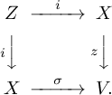
A well-known consequence of regularity of
 $\sigma $
is that this square is tor-independent.Footnote 8 Since
$\sigma $
is that this square is tor-independent.Footnote 8 Since
 $i_*$
is compatible with tor-independent base change (Lemma 4.6(2)), we deduce from Proposition 5.19 that
$i_*$
is compatible with tor-independent base change (Lemma 4.6(2)), we deduce from Proposition 5.19 that
 $$\begin{align*}e(V, \sigma, E) = \sigma^*z_*(1) = i_*i^*(1) = i_*(1). \end{align*}$$
This was to be shown.
It follows that, as explained in §3.4, both the ordinary and refined Euler numbers in E-cohomology can be computed as sums of local indices. The remainder of this paper is mainly concerned with determining these indices, for certain examples of E.
Remark 5.22. These results can be generalized slightly. Fix a scheme S and an
 $\mathrm {SL}$
-oriented ring spectrum
$\mathrm {SL}$
-oriented ring spectrum
 $E \in \mathcal {SH}(S)$
.
$E \in \mathcal {SH}(S)$
.
-
(1) Let
$X/S$
be smoothable lci and
$V/X$
a vector bundle, relatively oriented in the sense of Definition 1.5. If
$X/S$
is in addition proper, then we can transfer the Euler class along the structure morphism (see §4.2.4) as before to obtain an Euler number
$n(V, \rho , E) \in E^0(S)$
. More generally, without assuming
$X/S$
proper, given a section
$\sigma $
with zero scheme Z proper over S, we obtain the refined Euler number
$n(V, \sigma , \rho , E)$
. -
(2) Let
$X/S$
be arbitrary, V a vector bundle, and
$\sigma $
a section of V with zero scheme
$i: Z \to X$
, and suppose that i is a regular immersion (but
$\sigma $
need not be a nondegenerate section–i.e., Z could have higher dimension than expected). In this case there is an excess bundle
$\mathcal E = cok(N_{Z/X} \to V\rvert _Z)$
.Footnote 9 A straightforward adaptation of the proof of Corollary 5.21, using the excess intersection formula [Reference Déglise, Jin and Khan26, Proposition 3.3.4], shows that
$$\begin{align*}e(V, \sigma, E) = i_*(e(\mathcal E, E)). \end{align*}$$
-
(3) Putting everything together, let
$X/S$
be proper smoothable lci, V a relatively oriented vector bundle, and
$\sigma $
a section with zero scheme Z regularly immersed in X. Then Here the sum is over clopen components
$$\begin{align*}n(V, \rho, E) = \sum_{Z^{\prime} \subset Z} n\left(\mathcal E\rvert_{Z^{\prime}}, \rho^{\prime}, E\right). \end{align*}$$
$Z^{\prime }$
of Z, and
$\rho ^{\prime }$
denotes the induced relative orientation of
$\mathcal E$
. Note that if
$\sigma $
is nondegenerate on
$Z^{\prime }$
–that is,
$\mathcal E\rvert _{Z^{\prime }} = 0$
–then
$e(\mathcal E\rvert _{Z'}, E) = 1 \in E^0(Z')$
and
$n(\mathcal E\rvert _{Z'}, \rho ', E) = \mathrm {ind}_{Z'}(\sigma )$
as before.


6 d-Dimensional planes on complete intersections in projective space
6.1 Some Euler numbers of symmetric powers on Grassmannians
Grassmannians and flag varieties are smooth and proper over
 $\mathbb {Z}$
, and the Euler classes of many of their vector bundles have interesting interpretations in enumerative geometry. Computations over
$\mathbb {Z}$
, and the Euler classes of many of their vector bundles have interesting interpretations in enumerative geometry. Computations over
 $\mathbb {R}$
and
$\mathbb {R}$
and
 $\mathbb {C}$
are available in the literature in connection with enumerative results or accessible with localization techniques in equivariant cohomology [Reference Atiyah and Bott4]. The integrality of Euler classes, as in Theorem 5.11 and Proposition 5.4, can leverage such results to all fields. We do this now using the
$\mathbb {C}$
are available in the literature in connection with enumerative results or accessible with localization techniques in equivariant cohomology [Reference Atiyah and Bott4]. The integrality of Euler classes, as in Theorem 5.11 and Proposition 5.4, can leverage such results to all fields. We do this now using the
 $\mathbb {Z}[1/2]$
case of Theorem 5.11 and a characteristic class argument. This is independent of recent work [Reference Calmès, Dotto, Harpaz, Hebestreit, Land, Moi, Nardin, Nikolaus and Steimle18] on Hermitian K-theory over
$\mathbb {Z}[1/2]$
case of Theorem 5.11 and a characteristic class argument. This is independent of recent work [Reference Calmès, Dotto, Harpaz, Hebestreit, Land, Moi, Nardin, Nikolaus and Steimle18] on Hermitian K-theory over
 $\mathbb {Z}$
, and the characteristic class argument may be of some independent interest. One can alternatively deduce Corollary 6.3 from the
$\mathbb {Z}$
, and the characteristic class argument may be of some independent interest. One can alternatively deduce Corollary 6.3 from the
 $\mathbb {Z}$
case of Theorem 5.11 and [Reference Calmès, Dotto, Harpaz, Hebestreit, Land, Moi, Nardin, Nikolaus and Steimle18].
$\mathbb {Z}$
case of Theorem 5.11 and [Reference Calmès, Dotto, Harpaz, Hebestreit, Land, Moi, Nardin, Nikolaus and Steimle18].
Remark 6.1. Suppose X is a smooth, proper
 $\mathbb {Z}$
-scheme with geometrically connected fibers and
$\mathbb {Z}$
-scheme with geometrically connected fibers and
 $\mathrm {Pic} X$
torsion free–for example, X a Grassmannian or projective space. For a relatively orientable vector bundle
$\mathrm {Pic} X$
torsion free–for example, X a Grassmannian or projective space. For a relatively orientable vector bundle
 $V \to X$
defined over
$V \to X$
defined over
 $\mathbb {Z}$
, there are at most two isomorphism classes of relative orientations. Namely, by assumption, there is a line bundle
$\mathbb {Z}$
, there are at most two isomorphism classes of relative orientations. Namely, by assumption, there is a line bundle
 $L \to X$
and an isomorphism
$L \to X$
and an isomorphism
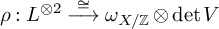 $\rho : L^{\otimes 2} \stackrel {\cong }{\longrightarrow } \omega _{X/\mathbb {Z}} \otimes \det V$
. Since
$\rho : L^{\otimes 2} \stackrel {\cong }{\longrightarrow } \omega _{X/\mathbb {Z}} \otimes \det V$
. Since
 $\mathrm {Pic} X$
is torsion free, any relative orientation is an isomorphism
$\mathrm {Pic} X$
is torsion free, any relative orientation is an isomorphism
 $L^{\otimes 2} \stackrel {\cong }{\longrightarrow } \omega _{X/\mathbb {Z}} \otimes \det V$
, whence two such differ by a global section of
$L^{\otimes 2} \stackrel {\cong }{\longrightarrow } \omega _{X/\mathbb {Z}} \otimes \det V$
, whence two such differ by a global section of
 $\operatorname {Hom}\left (L^{\otimes 2},L^{\otimes 2}\right ) \cong \mathcal {O}(X)^*$
. By hypothesis on X, the fibers of the push-forward of
$\operatorname {Hom}\left (L^{\otimes 2},L^{\otimes 2}\right ) \cong \mathcal {O}(X)^*$
. By hypothesis on X, the fibers of the push-forward of
 $\mathcal {O}_X$
all have rank
$\mathcal {O}_X$
all have rank
 $1$
, whence this push-forward is
$1$
, whence this push-forward is
 $\mathcal {O}_{\mathbb {Z}}$
and
$\mathcal {O}_{\mathbb {Z}}$
and
 $\mathcal {O}(X)^* \cong \mathbb {Z}^* = \{\pm 1\}$
. Thus any relative orientation is isomorphic to
$\mathcal {O}(X)^* \cong \mathbb {Z}^* = \{\pm 1\}$
. Thus any relative orientation is isomorphic to
 $\rho $
or
$\rho $
or
 $-\rho $
. We then have
$-\rho $
. We then have
 $n(V, \rho ) = \langle -1 \rangle n(V, -\rho )$
.
$n(V, \rho ) = \langle -1 \rangle n(V, -\rho )$
.
Consequently we suppress the choice of orientation and just write
 $n(V)$
. Beware that this does not mean that every vector bundle is relatively orientable, though!
$n(V)$
. Beware that this does not mean that every vector bundle is relatively orientable, though!
Remark 6.2. There is a canonical relative orientation for certain classes of vector bundles on Grassmannians
 $X = \operatorname {Gr}(d,n)$
: a point p of X with residue field L corresponds to a dimension
$X = \operatorname {Gr}(d,n)$
: a point p of X with residue field L corresponds to a dimension
 $d+1$
subspace of
$d+1$
subspace of
 $L^{n+1}$
. A choice of basis
$L^{n+1}$
. A choice of basis
 $\{e_0,\ldots ,e_n\}$
of
$\{e_0,\ldots ,e_n\}$
of
 $L^{n+1}$
such that the span of
$L^{n+1}$
such that the span of
 $\{e_0,\ldots ,e_d\}$
is p defines canonical local coordinates for an affine chart isomorphic to
$\{e_0,\ldots ,e_d\}$
is p defines canonical local coordinates for an affine chart isomorphic to
 $\mathbb A^{(n-d)(d+1)}$
with p as the origin (see, e.g., [Reference Kass and Wickelgren49, Definition 42]). This defines local trivializations of the tautological and quotient bundles on X, and therefore also of their tensor, symmetric, exterior powers, and their duals. A vector bundle V formed from such operations on the tautological and quotient bundles and which is relatively orientable on X inherits a canonical relative orientation
$\mathbb A^{(n-d)(d+1)}$
with p as the origin (see, e.g., [Reference Kass and Wickelgren49, Definition 42]). This defines local trivializations of the tautological and quotient bundles on X, and therefore also of their tensor, symmetric, exterior powers, and their duals. A vector bundle V formed from such operations on the tautological and quotient bundles and which is relatively orientable on X inherits a canonical relative orientation
 $\rho $
such that the local coordinates and trivializations just described are compatible with
$\rho $
such that the local coordinates and trivializations just described are compatible with
 $\rho $
in the sense of [Reference Kass and Wickelgren49, Definition 21]. This is described in [Reference Kass and Wickelgren49, Proposition 45] in a special case, but the argument holds in the stated generality. (One only needs the determinants of the clutching functions to be squares, which follows from the relative orientability of V. Together with the explicit coordinates, this gives the relative orienation.) This relative orientation has the property that it is defined over
$\rho $
in the sense of [Reference Kass and Wickelgren49, Definition 21]. This is described in [Reference Kass and Wickelgren49, Proposition 45] in a special case, but the argument holds in the stated generality. (One only needs the determinants of the clutching functions to be squares, which follows from the relative orientability of V. Together with the explicit coordinates, this gives the relative orienation.) This relative orientation has the property that it is defined over
 $\mathbb {Z}$
, and for any very nondegenerate section
$\mathbb {Z}$
, and for any very nondegenerate section
 $\sigma $
, the data just described give a system of coordinates in the sense of Definition 2.28.
$\sigma $
, the data just described give a system of coordinates in the sense of Definition 2.28.
Corollary 6.3. Let
 $d \leq n$
be positive integers, and let
$d \leq n$
be positive integers, and let
 $X=\operatorname {Gr}(d,n)$
be the Grassmannian of d-planes
$X=\operatorname {Gr}(d,n)$
be the Grassmannian of d-planes
 $\mathbb P^d$
in
$\mathbb P^d$
in
 $\mathbb P^n$
. Let
$\mathbb P^n$
. Let
 $V = \oplus _{i=1}^j \operatorname {Sym}^{n_i} \mathcal {S}^*$
, where
$V = \oplus _{i=1}^j \operatorname {Sym}^{n_i} \mathcal {S}^*$
, where
 $\mathcal {S}$
denotes the tautological bundle on X and
$\mathcal {S}$
denotes the tautological bundle on X and
 $n_1,\ldots ,n_j$
are positive integers such that
$n_1,\ldots ,n_j$
are positive integers such that
 $\operatorname {rank} V = \dim X$
and V is relatively orientable–that is, such that
$\operatorname {rank} V = \dim X$
and V is relatively orientable–that is, such that
 $\sum _{i=1}^j {n_i + d \choose d}= (d+1)(n-d) $
and
$\sum _{i=1}^j {n_i + d \choose d}= (d+1)(n-d) $
and
 $\sum _{i=1}^j \frac {n_i}{d+1}{n_i + d \choose d} + n+1$
is even. Then
$\sum _{i=1}^j \frac {n_i}{d+1}{n_i + d \choose d} + n+1$
is even. Then
 $$ \begin{align*}n(V) = \frac{ n_{\mathbb{C}} +n_{\mathbb{R}} }{2} + \frac{ n_{\mathbb{C}} -n_{\mathbb{R}} }{2}\langle -1 \rangle\end{align*} $$
over any ring in which
 $2$
is invertible (where we interpret
$2$
is invertible (where we interpret
 $n(V)$
as
$n(V)$
as
 $n(V,KO)$
) or any field (where we interpret
$n(V,KO)$
) or any field (where we interpret
 $n(V)$
as
$n(V)$
as
 $n^{\mathrm {GS}}(V)$
).
$n^{\mathrm {GS}}(V)$
).
Proof. Let
 $\mathcal {O}(1)$
denote the generator of
$\mathcal {O}(1)$
denote the generator of
 $\mathrm {Pic} X$
given by the pullback of the tautological bundle under the Plücker embedding. Then
$\mathrm {Pic} X$
given by the pullback of the tautological bundle under the Plücker embedding. Then
 $\omega _{X/\mathbb {Z}} \cong \mathcal {O}(-n-1)$
and
$\omega _{X/\mathbb {Z}} \cong \mathcal {O}(-n-1)$
and
 $\det \operatorname {Sym}^{n_i} \mathcal {S}^* \cong \mathcal {O}\left (\frac {n_i}{d+1}{n_i + d \choose d}\right )$
. Thus V is relatively orientable as a bundle over
$\det \operatorname {Sym}^{n_i} \mathcal {S}^* \cong \mathcal {O}\left (\frac {n_i}{d+1}{n_i + d \choose d}\right )$
. Thus V is relatively orientable as a bundle over
 $\mathbb {Z}$
, and Remarks 6.1 and 6.2 apply.
$\mathbb {Z}$
, and Remarks 6.1 and 6.2 apply.
By the
 $\mathbb {Z}[1/2]$
case of Theorem 5.11, it is enough to show that the discriminant of
$\mathbb {Z}[1/2]$
case of Theorem 5.11, it is enough to show that the discriminant of
 $n\left (V_{\mathbb {F}_p}\right )$
is trivial for some prime p congruent to
$n\left (V_{\mathbb {F}_p}\right )$
is trivial for some prime p congruent to
 $1$
mod
$1$
mod
 $4$
and such that
$4$
and such that
 $2$
is not a square (see Remark 5.12). Let
$2$
is not a square (see Remark 5.12). Let
 $\mathrm {EM}(\mathrm {W})$
denote the Eilenberg–MacLane spectrum of the
$\mathrm {EM}(\mathrm {W})$
denote the Eilenberg–MacLane spectrum of the
 $\eta $
-inverted Milnor–Witt sheaves
$\eta $
-inverted Milnor–Witt sheaves
 $\mathrm {K}^{\mathrm {MW}}_*\left [\eta ^{-1}\right ]$
(compare [Reference Levine54, Remark 3.1]), and consider the associated Euler class
$\mathrm {K}^{\mathrm {MW}}_*\left [\eta ^{-1}\right ]$
(compare [Reference Levine54, Remark 3.1]), and consider the associated Euler class
 $e(V,\mathrm {EM}(\mathrm {W}))$
. Then
$e(V,\mathrm {EM}(\mathrm {W}))$
. Then
 $n(V,\mathrm {EM}(\mathrm {W}))$
determines the Witt class of
$n(V,\mathrm {EM}(\mathrm {W}))$
determines the Witt class of
 $n(V)$
, and hence the discriminant of
$n(V)$
, and hence the discriminant of
 $n(V)$
as well.
$n(V)$
as well.
d is even: Suppose that d is even. Let
 $\pi $
denote the structure map of X. Since
$\pi $
denote the structure map of X. Since
 $n(V,\mathrm {EM}(\mathrm {W})) = \pi _*\prod _{i=1}^j e(\operatorname {Sym}^{n_i} \mathcal {S}^*, \mathrm {EM}(\mathrm {W}))$
, it is enough to show that
$n(V,\mathrm {EM}(\mathrm {W})) = \pi _*\prod _{i=1}^j e(\operatorname {Sym}^{n_i} \mathcal {S}^*, \mathrm {EM}(\mathrm {W}))$
, it is enough to show that
 $e(\operatorname {Sym}^{n_1} \mathcal {S}^*, \mathrm {EM}(\mathrm {W})) =0$
. By the Jouanolou device, we may assume that any vector bundle is pulled back from the universal bundle. It is therefore enough to show the same for the dual tautological bundle on the universal Grassmannian
$e(\operatorname {Sym}^{n_1} \mathcal {S}^*, \mathrm {EM}(\mathrm {W})) =0$
. By the Jouanolou device, we may assume that any vector bundle is pulled back from the universal bundle. It is therefore enough to show the same for the dual tautological bundle on the universal Grassmannian
 $B\mathrm {GL}_{d+1}$
–that is, let
$B\mathrm {GL}_{d+1}$
–that is, let
 $\mathcal {S}_{d+1}^*$
denote the dual of the tautological bundle on
$\mathcal {S}_{d+1}^*$
denote the dual of the tautological bundle on
 $B\mathrm {GL}_{d+1}$
; we show that
$B\mathrm {GL}_{d+1}$
; we show that
 $e\left (\operatorname {Sym}^{n_1} \mathcal {S}_{d+1}^*, \mathrm {EM}(\mathrm {W})\right )=0$
. By Ananyevskiy’s splitting principle [Reference Ananyevskiy2, Theorem 6] and its extension due to M. Levine [Reference Levine54, Theorem 4.1], we may show the vanishing of the
$e\left (\operatorname {Sym}^{n_1} \mathcal {S}_{d+1}^*, \mathrm {EM}(\mathrm {W})\right )=0$
. By Ananyevskiy’s splitting principle [Reference Ananyevskiy2, Theorem 6] and its extension due to M. Levine [Reference Levine54, Theorem 4.1], we may show the vanishing of the
 $\mathrm {EM}(\mathrm {W})$
-Euler class of
$\mathrm {EM}(\mathrm {W})$
-Euler class of
 $\operatorname {Sym}^{n_1} \mathcal {S}_{d+1}^*$
after pullback to
$\operatorname {Sym}^{n_1} \mathcal {S}_{d+1}^*$
after pullback to
 $$ \begin{align*}B\mathrm{SL}_2 \times B\mathrm{SL}_2 \times \cdots \times B\mathrm{SL}_2 \times B\mathrm{SL}_1\end{align*} $$
via the map classifying the external Whitney sum of the tautological bundles. Here we use the fact that
 $d+1$
is odd. This pullback of
$d+1$
is odd. This pullback of
 $\operatorname {Sym}^{n_1} \mathcal {S}_{d+1}^*$
contains the odd-rank summand
$\operatorname {Sym}^{n_1} \mathcal {S}_{d+1}^*$
contains the odd-rank summand
 $\operatorname {Sym}^{n_1} \mathcal {S}_{1}^*$
, and therefore its
$\operatorname {Sym}^{n_1} \mathcal {S}_{1}^*$
, and therefore its
 $\mathrm {EM}(\mathrm {W})$
-Euler class is
$\mathrm {EM}(\mathrm {W})$
-Euler class is
 $0$
as desired (see [Reference Ananyevskiy2, Lemma 3] and [Reference Levine54, Lemma 4.3]).
$0$
as desired (see [Reference Ananyevskiy2, Lemma 3] and [Reference Levine54, Lemma 4.3]).
d is odd: Let k be a finite field whose order is prime to
 $2\prod _{i=1}^j (n_i)!$
, congruent to
$2\prod _{i=1}^j (n_i)!$
, congruent to
 $1$
mod
$1$
mod
 $4$
(so
$4$
(so
 $-1$
is a square), and such that
$-1$
is a square), and such that
 $2$
is not a square. By Theorem 5.11, it suffices to show that the discriminant of
$2$
is not a square. By Theorem 5.11, it suffices to show that the discriminant of
 $n(V,\operatorname {Gr}(d,n)) \in \mathrm {W}(k) \cong \mathrm {GW}(k)/\mathbb {Z}h$
is trivial (compare Remark 5.12).
$n(V,\operatorname {Gr}(d,n)) \in \mathrm {W}(k) \cong \mathrm {GW}(k)/\mathbb {Z}h$
is trivial (compare Remark 5.12).
Define r in
 $\mathbb {Z}$
such that
$\mathbb {Z}$
such that
 $d=2r+1$
. Let
$d=2r+1$
. Let
 $S_{d+1}^*$
denote the dual tautological bundle on
$S_{d+1}^*$
denote the dual tautological bundle on
 $B\mathrm {SL}_{d+1}$
and let
$B\mathrm {SL}_{d+1}$
and let
 $p_1,\ldots ,p_r,p_{r+1}$
and e in
$p_1,\ldots ,p_r,p_{r+1}$
and e in
 $\mathrm {EM}(\mathrm {W})^*\left (B\mathrm {SL}_{d+1}\right ) $
denote its Pontryagin and Euler classes, respectively. (Often one would let
$\mathrm {EM}(\mathrm {W})^*\left (B\mathrm {SL}_{d+1}\right ) $
denote its Pontryagin and Euler classes, respectively. (Often one would let
 $p_i$
be the Pontryagin classes of the tautological bundle, not its dual, but this is more convenient here.) By Lemma 6.5,
$p_i$
be the Pontryagin classes of the tautological bundle, not its dual, but this is more convenient here.) By Lemma 6.5,
 $e\left (\operatorname {Sym}^{n_i} S_{d+1}^*, \mathrm {EM}(\mathrm {W})\right )$
is in the image of
$e\left (\operatorname {Sym}^{n_i} S_{d+1}^*, \mathrm {EM}(\mathrm {W})\right )$
is in the image of
 $\mathbb {Z}[p_1,\ldots ,p_r,e] \to \mathrm {EM}(\mathrm {W})^*\left (B\mathrm {SL}_{d+1}\right )$
. (Note that we have omitted
$\mathbb {Z}[p_1,\ldots ,p_r,e] \to \mathrm {EM}(\mathrm {W})^*\left (B\mathrm {SL}_{d+1}\right )$
. (Note that we have omitted
 $p_{r+1}$
, as
$p_{r+1}$
, as
 $p_{r+1} = e^2$
[Reference Ananyevskiy2, Corollary 3].) Therefore
$p_{r+1} = e^2$
[Reference Ananyevskiy2, Corollary 3].) Therefore
 $e(V,\operatorname {Gr}(d,n))$
can be expressed as a polynomial with integer coefficients in the Pontryagin classes and Euler class of the dual tautological bundle
$e(V,\operatorname {Gr}(d,n))$
can be expressed as a polynomial with integer coefficients in the Pontryagin classes and Euler class of the dual tautological bundle
 $\mathcal {S}^*$
on
$\mathcal {S}^*$
on
 $\operatorname {Gr}(d,n)$
. By Lemma 6.7, it follows that
$\operatorname {Gr}(d,n)$
. By Lemma 6.7, it follows that
 $\operatorname {disc} n(V,\operatorname {Gr}(d,n))=1$
in
$\operatorname {disc} n(V,\operatorname {Gr}(d,n))=1$
in
 $k^*/(k^*)^2$
as desired.
$k^*/(k^*)^2$
as desired.
M. Levine [Reference Levine54] uses the normalizer N of the standard torus of
 $\mathrm {SL}_{2}$
,
$\mathrm {SL}_{2}$
,
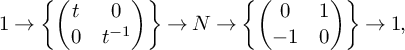 $$ \begin{align*}1 \to \left\{\begin{pmatrix} t & 0 \\ 0 & t^{-1} \end{pmatrix} \right\} \to N \to \left\{\begin{pmatrix} 0 & 1 \\ -1 & 0 \end{pmatrix} \right\} \to 1,\end{align*} $$
and bundles
 $\tilde {O}(a)$
and
$\tilde {O}(a)$
and
 $\tilde {O}^{-}(a)$
for a in
$\tilde {O}^{-}(a)$
for a in
 $\mathbb {Z}$
corresponding respectively to the representations
$\mathbb {Z}$
corresponding respectively to the representations
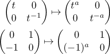 $$ \begin{align*}\begin{pmatrix} t & 0 \\ 0 & t^{-1} \end{pmatrix} \mapsto \begin{pmatrix} t^a & 0 \\ 0 & t^{-a} \end{pmatrix} \\ \begin{pmatrix} 0 & 1 \\ -1 & 0 \end{pmatrix} \mapsto \begin{pmatrix} 0 & 1 \\ (-1)^a & 0 \end{pmatrix} \end{align*} $$
and
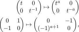 $$ \begin{align*}\begin{pmatrix} t & 0 \\ 0 & t^{-1} \end{pmatrix} \mapsto \begin{pmatrix} t^a & 0 \\ 0 & t^{-a} \end{pmatrix} \\ \begin{pmatrix} 0 & 1 \\ -1 & 0 \end{pmatrix} \mapsto \begin{pmatrix} 0 & -1 \\ (-1)^{a+1} & 0 \end{pmatrix}, \end{align*} $$
to compute characteristic classes, and we use his technique. We will use the notation
 $\tilde {O}^{(-)} (a)$
to mean either
$\tilde {O}^{(-)} (a)$
to mean either
 $\tilde {O}(a)$
or
$\tilde {O}(a)$
or
 $\tilde {O}^{-}(a)$
when a claim holds for both possibilities. We likewise use the
$\tilde {O}^{-}(a)$
when a claim holds for both possibilities. We likewise use the
 $\mathrm {EM}(\mathrm {W})$
-Pontryagin (or Borel) classes of a vector bundle with trivialized determinant of Panin and Walter [Reference Panin and Walter64]. For background on these classes, see [Reference Ananyevskiy2, Introduction, Section 3], [Reference Levine54, Section 3], or [Reference Wendt74, Section 2].
$\mathrm {EM}(\mathrm {W})$
-Pontryagin (or Borel) classes of a vector bundle with trivialized determinant of Panin and Walter [Reference Panin and Walter64]. For background on these classes, see [Reference Ananyevskiy2, Introduction, Section 3], [Reference Levine54, Section 3], or [Reference Wendt74, Section 2].
Let
 $e_i \in \mathrm {EM}(\mathrm {W})^*\left (N^{r+1}\right )$
denote the pullback of
$e_i \in \mathrm {EM}(\mathrm {W})^*\left (N^{r+1}\right )$
denote the pullback of
 $e\left (S_{2}^* ,\mathrm {EM}(\mathrm {W})\right )$
under the ith projection
$e\left (S_{2}^* ,\mathrm {EM}(\mathrm {W})\right )$
under the ith projection
 $BN^{r+1} \to BN$
composed with the canonical map
$BN^{r+1} \to BN$
composed with the canonical map
 $BN \to B\mathrm {SL}_2$
.
$BN \to B\mathrm {SL}_2$
.
Given vector bundles V and E on schemes X and Y, respectively, let
 $V \boxtimes E$
denote the vector bundle on
$V \boxtimes E$
denote the vector bundle on
 $X \times Y$
given by the tensor product of the pullbacks of V and E.
$X \times Y$
given by the tensor product of the pullbacks of V and E.
Lemma 6.4. Suppose
 $r \geq 1$
and
$r \geq 1$
and
 $a_1,\ldots ,a_{r+1}$
are integers, and that our base scheme is a field k with characteristic not dividing
$a_1,\ldots ,a_{r+1}$
are integers, and that our base scheme is a field k with characteristic not dividing
 $2 \prod _{i=1}^{r+1} a_i$
. The Euler class
$2 \prod _{i=1}^{r+1} a_i$
. The Euler class
 $e\left ( \boxtimes _{i=1}^{r+1} \tilde {O}^{(-)} (a_i), \mathrm {EM}(\mathrm {W})\right )$
and
$e\left ( \boxtimes _{i=1}^{r+1} \tilde {O}^{(-)} (a_i), \mathrm {EM}(\mathrm {W})\right )$
and
 $\mathrm {EM}(\mathrm {W})$
-Pontryagin classes
$\mathrm {EM}(\mathrm {W})$
-Pontryagin classes
 $p_j\left (\boxtimes _{i=1}^{r+1} \tilde {O}^{(-)} (a_i), \mathrm {EM}(\mathrm {W})\right )$
for
$p_j\left (\boxtimes _{i=1}^{r+1} \tilde {O}^{(-)} (a_i), \mathrm {EM}(\mathrm {W})\right )$
for
 $j=1,\ldots , 2^r$
are in the image of the map
$j=1,\ldots , 2^r$
are in the image of the map
 $$ \begin{align*}\mathbb{Z}\left[e_1^2,\ldots, e_{r+1}^2\right] \to \mathrm{EM}(\mathrm{W})^*\left(BN^{r+1}\right).\end{align*} $$
Proof. Proceed by induction on r. By Ananyevskiy’s splitting principle [Reference Ananyevskiy2, Theorem 6], there exists a map
 $\pi :Y \to BN^{r}$
such that the pullback of
$\pi :Y \to BN^{r}$
such that the pullback of
 $\boxtimes _{i=2}^{r+1} \tilde {O}^{(-)} (a_i)$
is a direct sum of rank
$\boxtimes _{i=2}^{r+1} \tilde {O}^{(-)} (a_i)$
is a direct sum of rank
 $2$
bundles
$2$
bundles
 $V_i$
on Y,
$V_i$
on Y,
 $$ \begin{align*}\pi^* \boxtimes_{i=2}^{r+1} \tilde{O}^{(-)} (a_i) \cong \oplus_{i=1}^{2^{r-1}} V_i,\end{align*} $$
and the map
 $$ \begin{align*}\mathrm{EM}(\mathrm{W})^*(BN \times BN^{r}) \to \mathrm{EM}(\mathrm{W})^*(BN \times Y)\end{align*} $$
is injective. We pull back the vector bundle
 $\boxtimes _{i=1}^{r+1} \tilde {O}^{(-)} (a_i)$
along the map
$\boxtimes _{i=1}^{r+1} \tilde {O}^{(-)} (a_i)$
along the map
 $1_{BN} \times \pi : BN \times Y \to BN^{r+1}$
and obtain an isomorphism
$1_{BN} \times \pi : BN \times Y \to BN^{r+1}$
and obtain an isomorphism
 $$ \begin{align}(1_{BN} \times \pi)^* \boxtimes_{i=1}^{r+1} \tilde{O}^{(-)} (a_i) \cong \oplus_{i=1}^{2^{r-1}} \left(\tilde{O}^{(-)} (a_1) \boxtimes V_i\right).\end{align} $$
By [Reference Levine54, Theorem 7.1] and the equality
 $e(S_{2},\mathrm {EM}(\mathrm {W}))^2 = e\left (S_{2}^*,\mathrm {EM}(\mathrm {W})\right )^2$
, which follows from [Reference Levine55, Theorem 11.1],
$e(S_{2},\mathrm {EM}(\mathrm {W}))^2 = e\left (S_{2}^*,\mathrm {EM}(\mathrm {W})\right )^2$
, which follows from [Reference Levine55, Theorem 11.1],
 $$ \begin{align} e\left(\tilde{O}^{(-)} (a_1),\mathrm{EM}(\mathrm{W})\right)^2 = a_1^2 e\left(S_{2}^*,\mathrm{EM}(\mathrm{W})\right)^2. \end{align} $$
Since
 $\tilde {O}^{(-)} (a_1)$
and
$\tilde {O}^{(-)} (a_1)$
and
 $V_i$
both have rank
$V_i$
both have rank
 $2$
, [Reference Levine54, Proposition 9.1] and equation (9) imply that
$2$
, [Reference Levine54, Proposition 9.1] and equation (9) imply that
 $$ \begin{align}e\left(\tilde{O}^{(-)} (a_1) \boxtimes V_i ,\mathrm{EM}(\mathrm{W})\right) = a_1^2 e_1^2 - e(V_i, \mathrm{EM}(\mathrm{W}))^2\end{align} $$
and
 $$ \begin{align}p_1\left(\tilde{O}^{(-)} (a_1) \boxtimes V_i ,\mathrm{EM}(\mathrm{W})\right) = 2\left(a_1^2 e_1^2 + e(V_i, \mathrm{EM}(\mathrm{W}))^2\right).\end{align} $$
This establishes the claim when
 $r=1$
, because
$r=1$
, because
 $p_2=e^2$
.
$p_2=e^2$
.
We now assume the claim holds for
 $r-1$
. By formula (8),
$r-1$
. By formula (8),
 $$ \begin{align}e\left((1_{BN} \times \pi)^* \boxtimes_{i=1}^{r+1} \tilde{O}^{(-)} (a_i), \mathrm{EM}(\mathrm{W})\right) = \prod_{i=1}^{2^{r-1}} e\left(\tilde{O}^{(-)} (a_1) \boxtimes V_i, \mathrm{EM}(\mathrm{W})\right) \end{align} $$
and
 $$ \begin{align}p\left((1_{BN} \times \pi)^* \boxtimes_{i=1}^{r+1} \tilde{O}^{(-)} (a_i), \mathrm{EM}(\mathrm{W})\right) = \prod_{i=1}^{2^{r-1}} p\left(\tilde{O}^{(-)} (a_1) \boxtimes V_i, \mathrm{EM}(\mathrm{W})\right),\end{align} $$
where p denotes the total Pontryagin class.
Combining equations (10) and (12) shows that
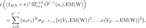 $$ \begin{align*}& e\left((1_{BN} \times \pi)^* \boxtimes_{i=1}^{r+1} \tilde{O}^{(-)} (a_i), \mathrm{EM}(\mathrm{W})\right)\\ &\quad= \sum_{i=0}^{2^{r-1}} (a_1 e_1)^{2i} \sigma_{2^{r-1} - i} \left( e(V_1, \mathrm{EM}(\mathrm{W}))^2, \ldots, e(V_{2^{r-1}}, \mathrm{EM}(\mathrm{W}))^2\right),\end{align*} $$
where
 $\sigma _i$
denotes the ith elementary symmetric function. Since the
$\sigma _i$
denotes the ith elementary symmetric function. Since the
 $V_i$
have rank
$V_i$
have rank
 $2$
,
$2$
,
 $$ \begin{align*}e(V_1, \mathrm{EM}(\mathrm{W}))^2 = p_1(V_1, \mathrm{EM}(\mathrm{W})),\end{align*} $$
and the Whitney sum formula for Pontryagin classes implies that
 $$ \begin{align*}p_{i} \left(\oplus_{j=1}^{2^{r-1}} V_i, \mathrm{EM}(\mathrm{W})\right) =\sigma_{i} \left( e(V_1, \mathrm{EM}(\mathrm{W}))^2, \ldots, e\left(V_{2^{r-1}}, \mathrm{EM}(\mathrm{W})\right)^2\right).\end{align*} $$
Since
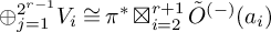 $\oplus _{j=1}^{2^{r-1}} V_i \cong \pi ^* \boxtimes _{i=2}^{r+1} \tilde {O}^{(-)} (a_i)$
, it follows by induction that
$\oplus _{j=1}^{2^{r-1}} V_i \cong \pi ^* \boxtimes _{i=2}^{r+1} \tilde {O}^{(-)} (a_i)$
, it follows by induction that
 $e\left ( \boxtimes _{i=1}^{r+1} \tilde {O}^{(-)} (a_i), \mathrm {EM}(\mathrm {W})\right )$
is in the image of
$e\left ( \boxtimes _{i=1}^{r+1} \tilde {O}^{(-)} (a_i), \mathrm {EM}(\mathrm {W})\right )$
is in the image of
 $\mathbb {Z}\left [e_1^2,\ldots , e_{r+1}^2\right ]$
.
$\mathbb {Z}\left [e_1^2,\ldots , e_{r+1}^2\right ]$
.
Combining equations (10), (11), and (13), we have
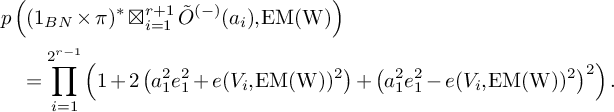 $$ \begin{align*}&p\left((1_{BN} \times \pi)^* \boxtimes_{i=1}^{r+1} \tilde{O}^{(-)} (a_i), \mathrm{EM}(\mathrm{W})\right)\\ &\quad= \prod_{i=1}^{2^{r-1}} \left(1+ 2\left(a_1^2 e_1^2 + e(V_i, \mathrm{EM}(\mathrm{W}))^2\right)+\left(a_1^2 e_1^2 - e(V_i, \mathrm{EM}(\mathrm{W}))^2\right)^2 \right).\end{align*} $$
Because the elementary symmetric polynomials generate all symmetric polynomials, it follows that
 $p\left ((1_{BN} \times \pi )^* \boxtimes _{i=1}^{r+1} \tilde {O}^{(-)} (a_i), \mathrm {EM}(\mathrm {W})\right ) $
is in the image of
$p\left ((1_{BN} \times \pi )^* \boxtimes _{i=1}^{r+1} \tilde {O}^{(-)} (a_i), \mathrm {EM}(\mathrm {W})\right ) $
is in the image of
 $$ \begin{align*}\mathbb{Z}\left[e_1^2, \sigma_{i} \left( e(V_1, \mathrm{EM}(\mathrm{W}))^2, \ldots, e\left(V_{2^{r-1}}, \mathrm{EM}(\mathrm{W})\right)^2\right): i = 1,\ldots, 2^{r-1}\right].\end{align*} $$
As before, these elementary symmetric functions are the Pontryagin classes of the pullback of
 $\boxtimes _{i=2}^{r+1} \tilde {O}^{(-)} (a_i)$
, finishing the proof by induction.
$\boxtimes _{i=2}^{r+1} \tilde {O}^{(-)} (a_i)$
, finishing the proof by induction.
Let
 $p_1,\ldots ,p_r$
and e in
$p_1,\ldots ,p_r$
and e in
 $\mathrm {EM}(\mathrm {W})^*\left (B\mathrm {SL}_{d+1}\right ) $
denote the Pontryagin and Euler classes, respectively, of the dual tautological bundle
$\mathrm {EM}(\mathrm {W})^*\left (B\mathrm {SL}_{d+1}\right ) $
denote the Pontryagin and Euler classes, respectively, of the dual tautological bundle
 $S_{d+1}^*$
on
$S_{d+1}^*$
on
 $B\mathrm {SL}_{d+1}$
.
$B\mathrm {SL}_{d+1}$
.
Lemma 6.5. Let
 $d = 2r+1$
be an odd integer and let n be a positive integer. Let k be a field of characteristic not dividing
$d = 2r+1$
be an odd integer and let n be a positive integer. Let k be a field of characteristic not dividing
 $2n!$
. Then
$2n!$
. Then
 $e\left (\operatorname {Sym}^{n} S_{d+1}^*, \mathrm {EM}(\mathrm {W})\right )$
is in the image of
$e\left (\operatorname {Sym}^{n} S_{d+1}^*, \mathrm {EM}(\mathrm {W})\right )$
is in the image of
 $\mathbb {Z}[p_1,\ldots ,p_r,e] \to \mathrm {EM}(\mathrm {W})^*\left (B\mathrm {SL}_{d+1}\right )$
.
$\mathbb {Z}[p_1,\ldots ,p_r,e] \to \mathrm {EM}(\mathrm {W})^*\left (B\mathrm {SL}_{d+1}\right )$
.
Proof. Let f denote the composite
 $$ \begin{align*}BN^{r+1} \to B\mathrm{SL}_{2}^{r+1} \to B\mathrm{SL}_{d+1}\end{align*} $$
of the
 $(r+1)$
-fold product of the canonical map
$(r+1)$
-fold product of the canonical map
 $BN \to B\mathrm {SL}_{2}$
with the map
$BN \to B\mathrm {SL}_{2}$
with the map
 $ B\mathrm {SL}_{2}^{r+1} \to B\mathrm {SL}_{d+1}$
classifying the external direct sum
$ B\mathrm {SL}_{2}^{r+1} \to B\mathrm {SL}_{d+1}$
classifying the external direct sum
 $\oplus _{i=1}^{r+1} S_2$
. There is an isomorphism
$\oplus _{i=1}^{r+1} S_2$
. There is an isomorphism
 $$ \begin{align}f^* \operatorname{Sym}^{n} S_{d+1}^* \cong \bigoplus_{\substack{\left(a_1,\ldots,a_{r+1}\right) \in \mathbb{Z}_{\geq 0}^{r+1} \\ \sum_i a_i = n}} \boxtimes_{i=1}^r \operatorname{Sym}^{a_i}\tilde{O}(1).\end{align} $$
By inspection, the symmetric powers of the tautological bundle
 $\tilde {O}(1)$
on
$\tilde {O}(1)$
on
 $BN$
split into a sum of bundles of rank
$BN$
split into a sum of bundles of rank
 $\leq 2$
(compare [Reference Levine54, p. Reference Graber and Pandharipande38]):
$\leq 2$
(compare [Reference Levine54, p. Reference Graber and Pandharipande38]):
 $$ \begin{align} \operatorname{Sym}^{a}\tilde{O}(1) \cong \begin{cases} \oplus_{l = 0}^b \tilde{O}^{(-1)^l} (i-2l) & \text{when } a= 2b+1 \text{ is odd},\\[3pt] \oplus_{l = 0}^{b-1} \tilde{O}^{(-1)^l} (i-2l) \oplus \mathcal{O} & \text{when } a = 2b \text{ is even and } b\text{ is even},\\[3pt] \oplus_{l = 0}^{b-1} \tilde{O}^{(-1)^l} (i-2l) \oplus \gamma & \text{when } a = 2b \text{ is even and } b\text{ is odd}, \end{cases} \end{align} $$
where
 $\gamma $
is the line bundle corresponding to the representation
$\gamma $
is the line bundle corresponding to the representation
 $N \to \mathrm {GL}_1$
sending the torus to
$N \to \mathrm {GL}_1$
sending the torus to
 $1$
and
$1$
and
 $\begin {pmatrix} 0 & 1 \\ -1 & 0 \end {pmatrix}$
to
$\begin {pmatrix} 0 & 1 \\ -1 & 0 \end {pmatrix}$
to
 $-1$
.
$-1$
.
Combining formulas (14) and (15), we can decompose
 $f^* \operatorname {Sym}^{n} S_{d+1}^*$
into a direct sum with summands which have various numbers of factors of rank
$f^* \operatorname {Sym}^{n} S_{d+1}^*$
into a direct sum with summands which have various numbers of factors of rank
 $2$
. Separate these summands into those with at least two rank
$2$
. Separate these summands into those with at least two rank
 $2$
factors and those with only one rank
$2$
factors and those with only one rank
 $2$
factor, if any of the latter sort appear. (This occurs when we can take all but one
$2$
factor, if any of the latter sort appear. (This occurs when we can take all but one
 $a_i$
to be even.) The direct sum of the latter such terms can alternatively be expressed as a sum of pullbacks of
$a_i$
to be even.) The direct sum of the latter such terms can alternatively be expressed as a sum of pullbacks of
 $\operatorname {Sym}^{a_i} \tilde {O}(1)$
under some projection
$\operatorname {Sym}^{a_i} \tilde {O}(1)$
under some projection
 $N^{r+1} \to N$
tensored with some
$N^{r+1} \to N$
tensored with some
 $\gamma $
s pulled back from other projections. We may ignore the factors of
$\gamma $
s pulled back from other projections. We may ignore the factors of
 $\gamma $
by [Reference Levine55, §10 p. 78 (2)], because
$\gamma $
by [Reference Levine55, §10 p. 78 (2)], because
 $e(\gamma ) = 0$
, as
$e(\gamma ) = 0$
, as
 $\gamma $
is a bundle of odd rank. Since
$\gamma $
is a bundle of odd rank. Since
 $\tilde {O}$
has rank
$\tilde {O}$
has rank
 $2$
and the characteristic of k does not divide
$2$
and the characteristic of k does not divide
 $2 a_i$
, we may apply [Reference Levine54, Theorem 8.1] and conclude that
$2 a_i$
, we may apply [Reference Levine54, Theorem 8.1] and conclude that
 $e\left (\operatorname {Sym}^{a_i} \tilde {O}(1)\right )$
is an integer multiple of a power of
$e\left (\operatorname {Sym}^{a_i} \tilde {O}(1)\right )$
is an integer multiple of a power of
 $e\left (\tilde {O}(1)\right )$
. Since the summands are symmetric under the permutation action of the symmetric group on
$e\left (\tilde {O}(1)\right )$
. Since the summands are symmetric under the permutation action of the symmetric group on
 $r+1$
letters on
$r+1$
letters on
 $B N^{r+1}$
, it follows that the Euler class of these summands is an integer multiple of a power of e.
$B N^{r+1}$
, it follows that the Euler class of these summands is an integer multiple of a power of e.
We now consider the Euler class of the rest of the summands. It suffices to show that the Euler class
 $\epsilon _1$
of the summands with at least two rank
$\epsilon _1$
of the summands with at least two rank
 $2$
factors is also in the image of
$2$
factors is also in the image of
 $\mathbb {Z}[p_1,\ldots ,p_r,e]$
. We may again ignore the factors of
$\mathbb {Z}[p_1,\ldots ,p_r,e]$
. We may again ignore the factors of
 $\gamma $
, as these do not change the Euler class. By Lemma 6.4,
$\gamma $
, as these do not change the Euler class. By Lemma 6.4,
 $\epsilon _1$
is the image of an element of
$\epsilon _1$
is the image of an element of
 $\mathbb {Z}\left [e_1^2,\ldots , e_{r+1}^2\right ]$
. Moreover, because each tuple
$\mathbb {Z}\left [e_1^2,\ldots , e_{r+1}^2\right ]$
. Moreover, because each tuple
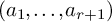 $\left (a_1, \ldots , a_{r+1} \right )$
of the direct sum occurs in every permutation, we may choose an element of
$\left (a_1, \ldots , a_{r+1} \right )$
of the direct sum occurs in every permutation, we may choose an element of
 $\mathbb {Z}\left [e_1^2,\ldots , e_{r+1}^2\right ] $
which is invariant under the permutation action of the symmetric group on
$\mathbb {Z}\left [e_1^2,\ldots , e_{r+1}^2\right ] $
which is invariant under the permutation action of the symmetric group on
 $r+1$
letters and which maps to
$r+1$
letters and which maps to
 $\epsilon _1$
. Thus,
$\epsilon _1$
. Thus,
 $\epsilon _1$
is in the image of the map
$\epsilon _1$
is in the image of the map
 $$ \begin{align*}\mathbb{Z}\left[\sigma_1\left(e_1^2,\ldots, e_{r+1}^2\right), \ldots, \sigma_{r+1}\left(e_1^2,\ldots, e_{r+1}^2\right)\right] \to \mathrm{EM}(\mathrm{W})^*\left(B N^{r+1}\right),\end{align*} $$
where
 $\sigma _i$
denotes the ith elementary symmetric polynomial. Since
$\sigma _i$
denotes the ith elementary symmetric polynomial. Since
 $\sigma _i\left (\left (e_1^2,\ldots , e_{r+1}^2\right )\right ) $
is the pullback to
$\sigma _i\left (\left (e_1^2,\ldots , e_{r+1}^2\right )\right ) $
is the pullback to
 $BN$
of
$BN$
of
 $p_i\left (S_{d+1}^* \to B\mathrm {SL}_{d+1}, \mathrm {EM}(\mathrm {W})\right )$
, we have that
$p_i\left (S_{d+1}^* \to B\mathrm {SL}_{d+1}, \mathrm {EM}(\mathrm {W})\right )$
, we have that
 $\epsilon _1$
is in the image of
$\epsilon _1$
is in the image of
 $\mathbb {Z}[p_1,\ldots ,p_r,e]$
, as desired.
$\mathbb {Z}[p_1,\ldots ,p_r,e]$
, as desired.
The Pontryagin and Euler classes of
 $\mathcal {S}_{d+1}^* \to \operatorname {Gr}(d,n)$
are pulled back from those of
$\mathcal {S}_{d+1}^* \to \operatorname {Gr}(d,n)$
are pulled back from those of
 $\mathcal {S}_{d+1}^* \to B\mathrm {GL}_{d+1}$
. The
$\mathcal {S}_{d+1}^* \to B\mathrm {GL}_{d+1}$
. The
 $\mathrm {EM}(\mathrm {W})^*$
-cohomology and twisted cohomology of
$\mathrm {EM}(\mathrm {W})^*$
-cohomology and twisted cohomology of
 $B\mathrm {GL}_{d+1}$
inject into that of
$B\mathrm {GL}_{d+1}$
inject into that of
 $B\mathrm {SL}_{d+1}$
,
$B\mathrm {SL}_{d+1}$
,
 $$ \begin{align*}\mathrm{EM}(\mathrm{W})^*\left(B\mathrm{GL}_{d+1}\right) \oplus \mathrm{EM}(\mathrm{W})^*\left(B\mathrm{GL}_{d+1}, \det \mathcal{S}\right) \subseteq \mathrm{EM}(\mathrm{W})^*\left(B\mathrm{SL}_{d+1}\right),\end{align*} $$
by [Reference Levine54, Theorem 4.1]. Under this injection, the Pontrygin and Euler classes of
 $\mathcal {S}_{d+1}^* \to B\mathrm {GL}_{d+1}$
are sent to
$\mathcal {S}_{d+1}^* \to B\mathrm {GL}_{d+1}$
are sent to
 $p_1, \ldots , p_r, p_{r+1}$
and to e, respectively, so we will let
$p_1, \ldots , p_r, p_{r+1}$
and to e, respectively, so we will let
 $p_i$
and e denote the corresponding characteristic classes of
$p_i$
and e denote the corresponding characteristic classes of
 $\mathcal {S}^* \to B\mathrm {GL}_{d+1}$
and
$\mathcal {S}^* \to B\mathrm {GL}_{d+1}$
and
 $\mathcal {S}_{d+1}^* \to \operatorname {Gr}(d,n)$
as well. Let
$\mathcal {S}_{d+1}^* \to \operatorname {Gr}(d,n)$
as well. Let
 $\pi : \operatorname {Gr}(d,n) \to \operatorname {Spec} k$
denote the structure map and
$\pi : \operatorname {Gr}(d,n) \to \operatorname {Spec} k$
denote the structure map and
 $$ \begin{align*}\pi_*: \mathrm{EM}(\mathrm{W})^*\left(\operatorname{Gr}(d,n), \left(\det \mathcal{S}_{d+1}^*\right)^{\otimes -(n+1)}\right)\to \mathrm{W}(k)\end{align*} $$
the induced push-forward on
 $\mathrm {EM}(\mathrm {W})^*$
-cohomology.
$\mathrm {EM}(\mathrm {W})^*$
-cohomology.
Lemma 6.6. Let
 $d = 2r+1$
be odd. For any nonnegative integers
$d = 2r+1$
be odd. For any nonnegative integers
 $a_1, \ldots , a_{r+1},b$
such that
$a_1, \ldots , a_{r+1},b$
such that
 $\sum (4i) a_i + b(d+1) = (d+1)(n-d)$
and
$\sum (4i) a_i + b(d+1) = (d+1)(n-d)$
and
 $b \equiv n+1 \ \ \mod 2$
, the monomial
$b \equiv n+1 \ \ \mod 2$
, the monomial
 $e^b \prod _{i=1}^{r+1} p_i^{a_i}$
in
$e^b \prod _{i=1}^{r+1} p_i^{a_i}$
in
 $\mathrm {EM}(\mathrm {W})^*\left (\operatorname {Gr}(d,n), \left (\det \mathcal {S}_{d+1}^* \right )^{\otimes b}\right )$
is in the image of
$\mathrm {EM}(\mathrm {W})^*\left (\operatorname {Gr}(d,n), \left (\det \mathcal {S}_{d+1}^* \right )^{\otimes b}\right )$
is in the image of
 $\mathbb {Z}[e]$
–or in other words, there exists c in
$\mathbb {Z}[e]$
–or in other words, there exists c in
 $\mathbb {Z}$
such that
$\mathbb {Z}$
such that
 $e^b \prod _{i=1}^{r+1} p_i^{a_i} = c e^{n-d}$
.
$e^b \prod _{i=1}^{r+1} p_i^{a_i} = c e^{n-d}$
.
Proof. Let Q denote the quotient bundle on
 $\operatorname {Gr}(d,n)$
, defined by the short exact sequence
$\operatorname {Gr}(d,n)$
, defined by the short exact sequence
 $$ \begin{align*}0 \to \mathcal{S}_{d+1} \to \mathcal{O}^{n+1} \to Q \to 0 .\end{align*} $$
In particular, the rank of Q is
 $n-d$
. The nonvanishing Pontryagin classes of
$n-d$
. The nonvanishing Pontryagin classes of
 $\mathcal {S}_{d+1}$
are
$\mathcal {S}_{d+1}$
are
 $p_1, \ldots , p_{r}, p_{r+1}$
, with
$p_1, \ldots , p_{r}, p_{r+1}$
, with
 $e^2 = p_{r+1}$
. Define s so that
$e^2 = p_{r+1}$
. Define s so that
 $n-d = 2s$
or
$n-d = 2s$
or
 $n-d=2s+1$
, depending on whether
$n-d=2s+1$
, depending on whether
 $n-d$
is odd or even. Let
$n-d$
is odd or even. Let
 $p_1^{\perp }, \ldots , p_s^{\perp } $
denote the nonvanishing Pontryagin classes of the dual to the quotient bundle
$p_1^{\perp }, \ldots , p_s^{\perp } $
denote the nonvanishing Pontryagin classes of the dual to the quotient bundle
 $Q^*$
on
$Q^*$
on
 $\operatorname {Gr}(d,n)$
. By [Reference Ananyevskiy2, Lemma 15],
$\operatorname {Gr}(d,n)$
. By [Reference Ananyevskiy2, Lemma 15],
 $$ \begin{align*}(1+p_1+ \cdots + p_{r+1})\left(1+ p_1^{\perp} + \cdots + p_s^{\perp}\right)=1\end{align*} $$
in
 $W^*(\operatorname {Gr}(d,n))$
. Setting the notation A for the ring
$W^*(\operatorname {Gr}(d,n))$
. Setting the notation A for the ring
 $$ \begin{align*}A = \mathbb{Z} \left[p_1, \ldots, p_{r}, p_{r+1}, p_1^{\perp}, \ldots, p_s^{\perp} \right]/\left\langle (1+p_1+ \cdots + p_{r} + p_{r+1})\left(1+ p_1^{\perp} + \cdots + p_s^{\perp}\right) - 1\right\rangle,\end{align*} $$
we therefore have a homomorphism
 $\tau : A \to \mathrm {EM}(\mathrm {W})^*(\operatorname {Gr}(d,n).$
There is a canonical isomorphism
$\tau : A \to \mathrm {EM}(\mathrm {W})^*(\operatorname {Gr}(d,n).$
There is a canonical isomorphism
 $$ \begin{align*}\mathrm{H}^*(\mathbb{C}\operatorname{Gr}(r,r+s); \mathbb{Z}) \cong A,\end{align*} $$
where
 $\mathrm {H}^*(\mathbb {C}\operatorname {Gr}(r,r+s); \mathbb {Z})$
denotes the singular cohomology of the
$\mathrm {H}^*(\mathbb {C}\operatorname {Gr}(r,r+s); \mathbb {Z})$
denotes the singular cohomology of the
 $\mathbb {C}$
-manifold associated to the
$\mathbb {C}$
-manifold associated to the
 $\mathbb {C}$
-points of the Grassmannian
$\mathbb {C}$
-points of the Grassmannian
 $\operatorname {Gr}(r,r+s)$
, sending the ith Chern class of the dual tautological bundle to
$\operatorname {Gr}(r,r+s)$
, sending the ith Chern class of the dual tautological bundle to
 $p_i$
. The top-dimensional singular cohomology
$p_i$
. The top-dimensional singular cohomology
 $\mathrm {H}^{(r+1)s}(\mathbb {C}\operatorname {Gr}(r,r+s); \mathbb {Z})$
is isomorphic to
$\mathrm {H}^{(r+1)s}(\mathbb {C}\operatorname {Gr}(r,r+s); \mathbb {Z})$
is isomorphic to
 $\mathbb {Z}$
by Poincaré duality. Under our chosen isomorphism, the monomial
$\mathbb {Z}$
by Poincaré duality. Under our chosen isomorphism, the monomial
 $p_{r+1}^s$
corresponds to the top Chern class
$p_{r+1}^s$
corresponds to the top Chern class
 $c_{(r+1)s}\left (\mathcal {S}_{r+1}^{\oplus s} \to \mathbb {C}\operatorname {Gr}(r,r+s)\right )$
of the direct sum of s-copies of the dual tautological bundle, which is a generator (with the usual
$c_{(r+1)s}\left (\mathcal {S}_{r+1}^{\oplus s} \to \mathbb {C}\operatorname {Gr}(r,r+s)\right )$
of the direct sum of s-copies of the dual tautological bundle, which is a generator (with the usual
 $\mathbb {C}$
-orientations,
$\mathbb {C}$
-orientations,
 $c_{(r+1)s}\left (\mathcal {S}_{r+1}^{\oplus s} \to \mathbb {C}\operatorname {Gr}(r,r+s)\right )$
counts the number of linear subspaces of dimension r in a complete intersection of s linear hypersurfaces in
$c_{(r+1)s}\left (\mathcal {S}_{r+1}^{\oplus s} \to \mathbb {C}\operatorname {Gr}(r,r+s)\right )$
counts the number of linear subspaces of dimension r in a complete intersection of s linear hypersurfaces in
 $\mathbb {C}\mathbb P^{r+s}$
, and this number is
$\mathbb {C}\mathbb P^{r+s}$
, and this number is
 $1$
; compare Remark 6.9 and Lemma 6.7). Therefore, for any monomial
$1$
; compare Remark 6.9 and Lemma 6.7). Therefore, for any monomial
 $\prod _{i=1}^{r+1} p_i^{a^{\prime }_i}$
with
$\prod _{i=1}^{r+1} p_i^{a^{\prime }_i}$
with
 $\sum _{i=1}^{r+1} ia^{\prime }_i = (r+1)s$
, there is an integer
$\sum _{i=1}^{r+1} ia^{\prime }_i = (r+1)s$
, there is an integer
 $c'$
such that
$c'$
such that
 $$ \begin{align} \prod_{i=1}^{r+1} p_i^{a^{\prime}_i} = c^{\prime} p_{r+1}^s\end{align} $$
in
 $\mathrm {H}^*(\mathbb {C}\operatorname {Gr}(r,r+s); \mathbb {Z}).$
Since d is odd,
 $n+1 \equiv n-d \ \ \mod 2$
, and therefore
$n+1 \equiv n-d \ \ \mod 2$
, and therefore
 $b \equiv n-d \ \ \mod 2$
. Note that if
$b \equiv n-d \ \ \mod 2$
. Note that if
 $n-d$
is odd,
$n-d$
is odd,
 $b \geq 0$
. We may then define a nonnegative integer
$b \geq 0$
. We may then define a nonnegative integer
 $b'$
by the rule
$b'$
by the rule
 $$ \begin{align*}b^{\prime} = \begin{cases} b/2 & \text{if } n-d \equiv 0 \ \ \mod 2,\\ (b-1)/2 & \text{if } n-d \equiv 1 \ \ \mod 2. \end{cases}\end{align*} $$
With this notation,
 $n-d-b= 2(s-b^{\prime })$
. Thus
$n-d-b= 2(s-b^{\prime })$
. Thus
 $$ \begin{align*}\sum (4i) a_i = (d+1)(n-d-b) = (d+1)2(s-b^{\prime}) = 4(r+1)(s-b'),\end{align*} $$
whence
 $$ \begin{align*}\sum i a_i = (r+1)(s-b').\end{align*} $$
By equation (16), there is an integer c such that we have the equality
 $$ \begin{align*}p_{r+1}^{b'}\prod_{i=1}^{r+1} p_i^{a_i} = c p_{r+1}^s \end{align*} $$
in
 $\mathrm {H}^*(\mathbb {C}\operatorname {Gr}(r,r+s); \mathbb {Z}).$
Applying
$\mathrm {H}^*(\mathbb {C}\operatorname {Gr}(r,r+s); \mathbb {Z}).$
Applying
 $\tau $
, we see that
$\tau $
, we see that
 $$ \begin{align*}e^{2b^{\prime}} \prod_{i=1}^{r+1} p_i^{a_i} = c' e^{2s},\end{align*} $$
which implies the claim, either immediately if
 $n-d$
is even or by multiplying by e if
$n-d$
is even or by multiplying by e if
 $n-d$
is odd.
$n-d$
is odd.
Lemma 6.7. Let d be odd. Suppose k is a finite field such that
 $-1$
is a square. For any nonnegative integers
$-1$
is a square. For any nonnegative integers
 $a_1,\ldots ,a_{r+1},b$
such that
$a_1,\ldots ,a_{r+1},b$
such that
 $b(d+1)+\sum _{i=1}^{r+1} 4i a_i= (d+1)(n-d)$
and
$b(d+1)+\sum _{i=1}^{r+1} 4i a_i= (d+1)(n-d)$
and
 $b \equiv n+1 \ \ \mod 2$
, the push-forward
$b \equiv n+1 \ \ \mod 2$
, the push-forward
 $\pi _*\left (e^b \prod _{i=1}^{r+1} p_i^{a_i}\right )$
has trivial discriminant.
$\pi _*\left (e^b \prod _{i=1}^{r+1} p_i^{a_i}\right )$
has trivial discriminant.
Remark 6.8. The condition
 $b \equiv n+1 \ \ \mod 2$
ensures that
$b \equiv n+1 \ \ \mod 2$
ensures that
 $e^b \prod _{i=1}^{r+1} p_i^{a_i}$
lies in the appropriate twist of the Witt cohomology of
$e^b \prod _{i=1}^{r+1} p_i^{a_i}$
lies in the appropriate twist of the Witt cohomology of
 $\operatorname {Gr}(d,n)$
–that is,
$\operatorname {Gr}(d,n)$
–that is,
 $e^b \prod _{i=1}^{r+1} p_i^{a_i}$
is in
$e^b \prod _{i=1}^{r+1} p_i^{a_i}$
is in
 $\mathrm {EM}(\mathrm {W})^*\left (\operatorname {Gr}(d,n),\omega _{\operatorname {Gr}\left (d,n\right )}/k\right )$
as opposed to
$\mathrm {EM}(\mathrm {W})^*\left (\operatorname {Gr}(d,n),\omega _{\operatorname {Gr}\left (d,n\right )}/k\right )$
as opposed to
 $\mathrm {EM}(\mathrm {W})^*(\operatorname {Gr}(d,n))$
, so that we may apply
$\mathrm {EM}(\mathrm {W})^*(\operatorname {Gr}(d,n))$
, so that we may apply
 $\pi _*$
. The condition on the sum
$\pi _*$
. The condition on the sum
 $b(d+1)+\sum _{i=1}^{r+1} 4i a_i$
ensures that
$b(d+1)+\sum _{i=1}^{r+1} 4i a_i$
ensures that
 $e^b \prod _{i=1}^{r+1} p_i^{a_i}$
lies in the
$e^b \prod _{i=1}^{r+1} p_i^{a_i}$
lies in the
 $(d+1)(n-d)$
-degree
$(d+1)(n-d)$
-degree
 $\mathrm {EM}(\mathrm {W})^*$
-cohomology of
$\mathrm {EM}(\mathrm {W})^*$
-cohomology of
 $\operatorname {Gr}(d,n)$
, so the codomain of
$\operatorname {Gr}(d,n)$
, so the codomain of
 $\pi _*$
is
$\pi _*$
is
 $\mathrm {W}(k)$
.
$\mathrm {W}(k)$
.
Proof. By Lemma 6.6, it suffices to show that
 $\operatorname {disc} \pi _*e^{n-d}=1$
. We may identify
$\operatorname {disc} \pi _*e^{n-d}=1$
. We may identify
 $\pi _*e^{n-d}$
with the Euler number of
$\pi _*e^{n-d}$
with the Euler number of
 $\oplus _{j=1}^{n-d} \mathcal {S}^*$
:
$\oplus _{j=1}^{n-d} \mathcal {S}^*$
:
 $$ \begin{align*}\pi_*e^{n-d} = n\left(\oplus_{j=1}^{n-d} \mathcal{S}^*, \mathrm{EM}(\mathrm{W})\right).\end{align*} $$
Let
 $x_0, \ldots , x_n$
be coordinates on a projective space
$x_0, \ldots , x_n$
be coordinates on a projective space
 $\mathbb P_k^n = \operatorname {Proj} k[x_0,\ldots , x_n]$
. The Euler number
$\mathbb P_k^n = \operatorname {Proj} k[x_0,\ldots , x_n]$
. The Euler number
 $ n\left (\oplus _{j=1}^{n-d} \mathcal {S}^*, \mathrm {EM}(\mathrm {W})\right ) $
can be calculated with the section
$ n\left (\oplus _{j=1}^{n-d} \mathcal {S}^*, \mathrm {EM}(\mathrm {W})\right ) $
can be calculated with the section
 $\sigma = \oplus _{i=d+1}^n x_i$
as in §2.4. There is an analogous section
$\sigma = \oplus _{i=d+1}^n x_i$
as in §2.4. There is an analogous section
 $\sigma _{\mathbb {Z}} = \oplus _{i=d+1}^n x_i$
of
$\sigma _{\mathbb {Z}} = \oplus _{i=d+1}^n x_i$
of
 $\oplus _{j=1}^{n-d} \mathcal {S}^*_{\mathbb {Z}} \to \operatorname {Gr}(d,n)_{\mathbb {Z}}$
defined over
$\oplus _{j=1}^{n-d} \mathcal {S}^*_{\mathbb {Z}} \to \operatorname {Gr}(d,n)_{\mathbb {Z}}$
defined over
 $\mathbb {Z}$
. The zero locus
$\mathbb {Z}$
. The zero locus
 $\sigma _{\mathbb {Z}} = 0$
is the single
$\sigma _{\mathbb {Z}} = 0$
is the single
 $\mathbb {Z}$
-point of the Grassmannian associated to the linear subspace of
$\mathbb {Z}$
-point of the Grassmannian associated to the linear subspace of
 $\mathbb P_k^n$
given by
$\mathbb P_k^n$
given by
 $x_{d+1} = x_{d+2} = \cdots = x_n = 0$
.
$x_{d+1} = x_{d+2} = \cdots = x_n = 0$
.
The vanishing locus of
 $\sigma _{\mathbb {Z}}$
is the origin of the affine space
$\sigma _{\mathbb {Z}}$
is the origin of the affine space
 $\mathbb A^{(d+1)(n-d)}_{\mathbb {Z}} = \operatorname {Spec} \mathbb {Z}\left [a_{ij}: i =0,\ldots , d, j=d+1,\ldots , n\right ] \hookrightarrow \operatorname {Gr}(d,n)$
whose point
$\mathbb A^{(d+1)(n-d)}_{\mathbb {Z}} = \operatorname {Spec} \mathbb {Z}\left [a_{ij}: i =0,\ldots , d, j=d+1,\ldots , n\right ] \hookrightarrow \operatorname {Gr}(d,n)$
whose point
 $\left (a_{ij}\right )$
corresponds to the row space of
$\left (a_{ij}\right )$
corresponds to the row space of
 $$ \begin{align} \begin{pmatrix} 1&0&\cdots & 0&a_{0,d+1} & a_{0,d+2} & \cdots & a_{0,n} \\ 0&1&\cdots & 0&a_{1,d+1} & a_{1,d+2} & \cdots & a_{1,n} \\ \vdots &\vdots &\ddots & \vdots &\vdots & \vdots & \ddots & \vdots \\ 0&0&\cdots & 1&a_{d,d+1} & a_{d,d+2} & \cdots & a_{d,n} \end{pmatrix}.\end{align} $$
For a description of these coordinates on this open affine of the Grassmannian, see, for example, [Reference Eisenbud and Harris28, Section 3.2]. Let
 $e_0,\ldots , e_n$
denote the standard basis of the free module of rank
$e_0,\ldots , e_n$
denote the standard basis of the free module of rank
 $n+1$
. Let
$n+1$
. Let
 $\tilde {e}_0,\ldots , \tilde {e}_n$
denote the basis consisting of the row space of matrix (17) followed by
$\tilde {e}_0,\ldots , \tilde {e}_n$
denote the basis consisting of the row space of matrix (17) followed by
 $e_{d+1},e_{d+1},\ldots ,e_{n}$
. Let
$e_{d+1},e_{d+1},\ldots ,e_{n}$
. Let
 $\tilde {x}_0,\ldots , \tilde {x}_n$
denote the dual basis to
$\tilde {x}_0,\ldots , \tilde {x}_n$
denote the dual basis to
 $\tilde {e}_0,\ldots , \tilde {e}_n$
. Over this
$\tilde {e}_0,\ldots , \tilde {e}_n$
. Over this
 $\mathbb A^{(d+1)(n-d)}_{\mathbb {Z}}$
, the vector bundle
$\mathbb A^{(d+1)(n-d)}_{\mathbb {Z}}$
, the vector bundle
 $\mathcal {S}^*_{\mathbb {Z}}$
is trivialized by the basis of sections
$\mathcal {S}^*_{\mathbb {Z}}$
is trivialized by the basis of sections
 $\left \{\tilde {x}_0,\ldots , \tilde {x}_d\right \}$
. Then we may interpret
$\left \{\tilde {x}_0,\ldots , \tilde {x}_d\right \}$
. Then we may interpret
 $\sigma $
as a function
$\sigma $
as a function
 $\mathbb A^{(d+1)(n-d)}_{\mathbb {Z}} \to \mathbb A^{(d+1)(n-d)}_{\mathbb {Z}}$
. Namely,
$\mathbb A^{(d+1)(n-d)}_{\mathbb {Z}} \to \mathbb A^{(d+1)(n-d)}_{\mathbb {Z}}$
. Namely,
 $$ \begin{align*}x_u \left(\left(a_{ij}\right)\right)= \sum_{l=0}^{d} \left(x_u\left(a_{ij}\right)\right)\left(\tilde{e_l}\right) \tilde{x}_l\end{align*} $$
for
 $$ \begin{align*}u = d+1, \ldots, n.\end{align*} $$
As a subscheme,
 $\sigma _{\mathbb {Z}} = 0$
is therefore the zero locus of
$\sigma _{\mathbb {Z}} = 0$
is therefore the zero locus of
 $$ \begin{align*}\left(x_u\left(a_{ij}\right)\right)\left(\tilde{e_l}\right) = a_{l,u}\end{align*} $$
for
 $l=0,\ldots , d$
and
$l=0,\ldots , d$
and
 $u = d+1, \ldots , n$
. Thus the subscheme of
$u = d+1, \ldots , n$
. Thus the subscheme of
 $\operatorname {Gr}(d,n)_{\mathbb {Z}}$
given by
$\operatorname {Gr}(d,n)_{\mathbb {Z}}$
given by
 $\{\sigma _{\mathbb {Z}} = 0\}$
is a section of the structure map
$\{\sigma _{\mathbb {Z}} = 0\}$
is a section of the structure map
 $\operatorname {Gr}(d,n)_{\mathbb {Z}} \to \operatorname {Spec} \mathbb {Z}$
. In particular, it is finite and étale of rank
$\operatorname {Gr}(d,n)_{\mathbb {Z}} \to \operatorname {Spec} \mathbb {Z}$
. In particular, it is finite and étale of rank
 $1$
. It follows that the Jacobian of
$1$
. It follows that the Jacobian of
 $\sigma $
,
$\sigma $
,
 $$ \begin{align*}\mathrm{Jac} \sigma \in \operatorname{Hom} \left(\det T\operatorname{Gr}(d,n)\rvert_{\left\{\sigma_{\mathbb{Z}} = 0\right\}}, \det \oplus_{j=1}^{n-d} \mathcal{S}^*_{\mathbb{Z}}\rvert_{\left\{\sigma_{\mathbb{Z}} = 0\right\}} \right)\end{align*} $$
(which is described further at the beginning of §6.2), is nowhere vanishing. Thus under the relative orientation
 $$ \begin{align*}\operatorname{Hom} \left(\det T\operatorname{Gr}(d,n), \det \oplus_{j=1}^{n-d} \mathcal{S}^*_{\mathbb{Z}} \right) \cong L^{\otimes 2},\end{align*} $$
we have that
 $\mathrm {Jac} \sigma $
is a nowhere-vanishing section of the restriction of
$\mathrm {Jac} \sigma $
is a nowhere-vanishing section of the restriction of
 $L^{\otimes 2}$
. Thus
$L^{\otimes 2}$
. Thus
 $\langle \mathrm {Jac} \sigma _{k} \rangle $
is either
$\langle \mathrm {Jac} \sigma _{k} \rangle $
is either
 $\langle -1 \rangle $
or
$\langle -1 \rangle $
or
 $\langle 1 \rangle $
; but
$\langle 1 \rangle $
; but
 $\langle -1 \rangle = 1$
by assumption. Since
$\langle -1 \rangle = 1$
by assumption. Since
 $n\left (\oplus _{j=1}^{n-d} \mathcal {S}_k^*, \mathrm {EM}(\mathrm {W})\right ) = \langle \mathrm {Jac} \sigma _{k} \rangle $
(compare Example 2.21), this proves the claim.
$n\left (\oplus _{j=1}^{n-d} \mathcal {S}_k^*, \mathrm {EM}(\mathrm {W})\right ) = \langle \mathrm {Jac} \sigma _{k} \rangle $
(compare Example 2.21), this proves the claim.
6.2 An arithmetic count of the d-planes on a complete intersection in projective space
A complete intersection of hypersurfaces
 $$ \begin{align*}X=\left\{F_1 =F_2 = \cdots = F_j=0\right\} \subset \mathbb{P}^n\end{align*} $$
with
 $F_i$
of degree
$F_i$
of degree
 $n_i$
gives rise to a section
$n_i$
gives rise to a section
 $\sigma $
of
$\sigma $
of
 $V= \oplus _{i=1}^j \operatorname {Sym}^{n_i} \mathcal {S}^*$
, defined by
$V= \oplus _{i=1}^j \operatorname {Sym}^{n_i} \mathcal {S}^*$
, defined by
 $\sigma (\mathbb {P}L) = \oplus _{i=1}^j F_i\rvert _L$
, where L is any (
$\sigma (\mathbb {P}L) = \oplus _{i=1}^j F_i\rvert _L$
, where L is any (
 $d+1$
)-dimensional linear subspace of
$d+1$
)-dimensional linear subspace of
 $\mathbb {A}^{n+1}$
containing the origin and
$\mathbb {A}^{n+1}$
containing the origin and
 $\mathbb {P}L$
denotes the corresponding point of
$\mathbb {P}L$
denotes the corresponding point of
 $\operatorname {Gr}(d,n)$
. The zeros of
$\operatorname {Gr}(d,n)$
. The zeros of
 $\sigma $
are then precisely the d-planes in X (see, e.g., [Reference Debarre and Manivel25]). By [Reference Debarre and Manivel25, Théorèye 2.1], the closed subscheme
$\sigma $
are then precisely the d-planes in X (see, e.g., [Reference Debarre and Manivel25]). By [Reference Debarre and Manivel25, Théorèye 2.1], the closed subscheme
 $\{ \sigma = 0\}$
of
$\{ \sigma = 0\}$
of
 $\operatorname {Gr}(d,n)$
is smooth for general X and either of the expected dimension
$\operatorname {Gr}(d,n)$
is smooth for general X and either of the expected dimension
 $(d+1)(n-d) - \operatorname {rank} V = (d+1)(n-d) - \sum _{i=1}^j {n_i + d \choose d}$
or empty, with the empty case occurring exactly when one or both of
$(d+1)(n-d) - \operatorname {rank} V = (d+1)(n-d) - \sum _{i=1}^j {n_i + d \choose d}$
or empty, with the empty case occurring exactly when one or both of
 $(d+1)(n-d) - \operatorname {rank} V$
and
$(d+1)(n-d) - \operatorname {rank} V$
and
 $n-2r-j$
is less than
$n-2r-j$
is less than
 $0$
. In particular, when
$0$
. In particular, when
 $(d+1)(n-d) - \operatorname {rank} V =0$
, the zeros of
$(d+1)(n-d) - \operatorname {rank} V =0$
, the zeros of
 $\sigma $
are isolated and étale over k for a general complete intersection X. The canonical relative orientation (Remark 6.2) of V determines an isomorphism
$\sigma $
are isolated and étale over k for a general complete intersection X. The canonical relative orientation (Remark 6.2) of V determines an isomorphism
 $\operatorname {Hom}(\det T\operatorname {Gr}(d,n), \det V) \cong L^{\otimes 2}$
for a line bundle L on
$\operatorname {Hom}(\det T\operatorname {Gr}(d,n), \det V) \cong L^{\otimes 2}$
for a line bundle L on
 $\operatorname {Gr}(d,n)$
. The Jacobian determinant
$\operatorname {Gr}(d,n)$
. The Jacobian determinant
 $\mathrm {Jac} \sigma $
at a zero p of
$\mathrm {Jac} \sigma $
at a zero p of
 $\sigma $
is an element of the fiber of the vector bundle
$\sigma $
is an element of the fiber of the vector bundle
 $\operatorname {Hom}(\det T\operatorname {Gr}(d,n), \det V)$
at p. Choosing any local trivialization of L, we have a well-defined element
$\operatorname {Hom}(\det T\operatorname {Gr}(d,n), \det V)$
at p. Choosing any local trivialization of L, we have a well-defined element
 $\mathrm {Jac} \Sigma (p)$
in
$\mathrm {Jac} \Sigma (p)$
in
 $k(p)/(k(p)^*)^2$
, which can also be computed by choosing a local trivialization of V and local coordinates of
$k(p)/(k(p)^*)^2$
, which can also be computed by choosing a local trivialization of V and local coordinates of
 $\operatorname {Gr}(d,n)$
compatible with the relative orientation and computing
$\operatorname {Gr}(d,n)$
compatible with the relative orientation and computing
 $\mathrm {Jac} \Sigma (p) = \det \left ( \frac {\partial \sigma _k}{\partial x_l} \right )$
.
$\mathrm {Jac} \Sigma (p) = \det \left ( \frac {\partial \sigma _k}{\partial x_l} \right )$
.
Corollary 6.9. Let
 $X=\left \{F_1 =F_2 = \cdots = F_j=0\right \} \subset \mathbb {P}^n$
be a general complete intersection of hypersurfaces
$X=\left \{F_1 =F_2 = \cdots = F_j=0\right \} \subset \mathbb {P}^n$
be a general complete intersection of hypersurfaces
 $F_i = 0$
of degree
$F_i = 0$
of degree
 $n_i$
in
$n_i$
in
 $\mathbb {P}^n_k$
a projective space over a field k. Suppose that
$\mathbb {P}^n_k$
a projective space over a field k. Suppose that
 $\sum _{i=1}^j {n_i + d \choose d}= (d+1)(n-d) $
and
$\sum _{i=1}^j {n_i + d \choose d}= (d+1)(n-d) $
and
 $\sum _{i=1}^j \frac {n_i}{d+1}{n_i + d \choose d} + n+1$
is even. Then
$\sum _{i=1}^j \frac {n_i}{d+1}{n_i + d \choose d} + n+1$
is even. Then
 $$ \begin{align*}\sum_{d\text{-planes } \mathbb{P}L \text{ in }X} \mathrm{tr}_{k(\mathbb{P}L)/k} \langle \mathrm{Jac}\sigma(\mathbb{P}L) \rangle = \frac{ n_{\mathbb{C}} +n_{\mathbb{R}} }{2} + \frac{n_{\mathbb{C}} + n_{\mathbb{R}}}{2}\langle -1 \rangle,\end{align*} $$
where
-
•
$k(\mathbb {P}L)$
denotes the residue field of
$\mathbb {P}L$
viewed as a point on the Grassmannian; -
•
$n_{\mathbb {C}}$
(resp.,
$n_{\mathbb {R}}$
) is the topological Euler number of the complex (resp., real) vector bundle associated to the algebraic vector bundle
$V= \oplus _{i=1}^j \operatorname {Sym}^{n_i} \mathcal {S}^*$
given the canonical relative orientation (Remark 6.2); and -
•
$\mathrm {Jac} \sigma $
is the Jacobian determinant.


Proof. By [Reference Debarre and Manivel25, Théorème 2.1], the zeros of
 $\sigma $
are isolated and étale over k. It follows [Reference Kass and Wickelgren49, p.18, Proposition 34] that for a zero of
$\sigma $
are isolated and étale over k. It follows [Reference Kass and Wickelgren49, p.18, Proposition 34] that for a zero of
 $\sigma $
corresponding to the d-plane
$\sigma $
corresponding to the d-plane
 $\mathbb {P}L$
, the local index is computed as
$\mathbb {P}L$
, the local index is computed as
 $\mathrm {ind}^{\mathrm {PH}}_{\mathbb {P}L} \sigma = \mathrm {tr}_{k(L)/k} \langle \mathrm {Jac}\sigma (\mathbb {P}L) \rangle $
(see §2.4 for the definition of the notation
$\mathrm {ind}^{\mathrm {PH}}_{\mathbb {P}L} \sigma = \mathrm {tr}_{k(L)/k} \langle \mathrm {Jac}\sigma (\mathbb {P}L) \rangle $
(see §2.4 for the definition of the notation
 $\mathrm {ind}^{\mathrm {PH}}$
). Thus
$\mathrm {ind}^{\mathrm {PH}}$
). Thus
 $ n^{\mathrm {PH}}(V, \sigma ) = \sum _{d\text {-planes } \mathbb {P}L \text { in }X} \mathrm {tr}_{k(L)/k} \langle \mathrm {Jac}\sigma (\mathbb {P}L) \rangle $
by Definition 2.24. Corollary 6.3 computes
$ n^{\mathrm {PH}}(V, \sigma ) = \sum _{d\text {-planes } \mathbb {P}L \text { in }X} \mathrm {tr}_{k(L)/k} \langle \mathrm {Jac}\sigma (\mathbb {P}L) \rangle $
by Definition 2.24. Corollary 6.3 computes
 $ n^{\mathrm {PH}}(V, \sigma )$
. Proposition 5.9 shows that
$ n^{\mathrm {PH}}(V, \sigma )$
. Proposition 5.9 shows that
 $n_{\mathbb {R}}$
and
$n_{\mathbb {R}}$
and
 $n_{\mathbb {C}}$
are the claimed topological Euler numbers.
$n_{\mathbb {C}}$
are the claimed topological Euler numbers.
Remark 6.10. Note that Corollary 6.9 is a weighted count of the dimension d hyperplanes on the complete intersection X, depending only on
 $n_1,\ldots ,n_j$
and not on the choice of polynomials
$n_1,\ldots ,n_j$
and not on the choice of polynomials
 $F_1,\ldots , F_j$
as long as these are chosen generally.
$F_1,\ldots , F_j$
as long as these are chosen generally.
Example 6.11. Examples where Corollary 6.9 applies include lines on a degree
 $2n-1$
hypersurface of dimension n,
$2n-1$
hypersurface of dimension n,
 $3$
-planes on a degree d hypersurface of dimension
$3$
-planes on a degree d hypersurface of dimension
 $2 + \frac {1}{3}{d+3 \choose 3}$
when this is an integer, and lines on a complete intersection of two degree
$2 + \frac {1}{3}{d+3 \choose 3}$
when this is an integer, and lines on a complete intersection of two degree
 $n-2$
polynomials in
$n-2$
polynomials in
 $\mathbb {P}^n$
for n odd.
$\mathbb {P}^n$
for n odd.
Matthias Wendt’s oriented Schubert calculus shows that enriched intersections of Schubert varieties are determined by the
 $\mathbb {R}$
and
$\mathbb {R}$
and
 $\mathbb {C}$
realizations in the same manner [Reference Wendt74, Theorem 8.6], as well as giving enumerative applications [Reference Wendt74, Section 9].
$\mathbb {C}$
realizations in the same manner [Reference Wendt74, Theorem 8.6], as well as giving enumerative applications [Reference Wendt74, Section 9].
For
 $d=j=1$
and
$d=j=1$
and
 $n_1=3$
, Corollary 6.3 is work of Kass and the second author [Reference Kass and Wickelgren49] over a general field. For
$n_1=3$
, Corollary 6.3 is work of Kass and the second author [Reference Kass and Wickelgren49] over a general field. For
 $d=1$
and general j and
$d=1$
and general j and
 $n_i$
, it is work of M. Levine [Reference Levine54] over a perfect field of characteristic either
$n_i$
, it is work of M. Levine [Reference Levine54] over a perfect field of characteristic either
 $0$
or prime to
$0$
or prime to
 $2$
and the odd
$2$
and the odd
 $n_i$
s. Our result eliminates the assumption on the characteristic and generalizes to arbitrary relatively orientable
$n_i$
s. Our result eliminates the assumption on the characteristic and generalizes to arbitrary relatively orientable
 $d,n,n_1,\ldots ,n_j$
.
$d,n,n_1,\ldots ,n_j$
.
In order to obtain an enumerative theorem whose statement is independent of
 $\mathbb A^1$
-homotopy theory, one needs an arithmetic-geometric interpretation of the local indices:
$\mathbb A^1$
-homotopy theory, one needs an arithmetic-geometric interpretation of the local indices:
Question 6.12. Can the local indices
 $\mathrm {ind}^{\mathrm {PH}}_{\mathbb {P}L} \sigma = \mathrm {tr}_{k(L)/k} \langle \mathrm {Jac}\sigma (\mathbb {P}L) \rangle $
be expressed in terms of the arithmetic geometry of the d-plane
$\mathrm {ind}^{\mathrm {PH}}_{\mathbb {P}L} \sigma = \mathrm {tr}_{k(L)/k} \langle \mathrm {Jac}\sigma (\mathbb {P}L) \rangle $
be expressed in terms of the arithmetic geometry of the d-plane
 $\mathbb {P}L$
on X?
$\mathbb {P}L$
on X?
Such expressions are available over
 $\mathbb {R}$
for
$\mathbb {R}$
for
 $d=j=1$
[Reference Finashin and Kharlamov36], and over a field k of characteristic not
$d=j=1$
[Reference Finashin and Kharlamov36], and over a field k of characteristic not
 $2$
for lines on a cubic surface [Reference Kass and Wickelgren49], lines on a quintic
$2$
for lines on a cubic surface [Reference Kass and Wickelgren49], lines on a quintic
 $3$
-fold [Reference Pauli66], and points on a complete intersection of hypersurfaces [Reference McKean58]. S. Pauli has interesting observations on such results for lines on the complete intersection of two cubics in
$3$
-fold [Reference Pauli66], and points on a complete intersection of hypersurfaces [Reference McKean58]. S. Pauli has interesting observations on such results for lines on the complete intersection of two cubics in
 $\mathbb P^5$
: dropping the assumption that the zeros of
$\mathbb P^5$
: dropping the assumption that the zeros of
 $\sigma $
are isolated, she computes contributions from infinite families of lines on a quintic
$\sigma $
are isolated, she computes contributions from infinite families of lines on a quintic
 $3$
-fold in some cases [Reference Pauli66]. An alternative point of view in terms of (S)pin structures for
$3$
-fold in some cases [Reference Pauli66]. An alternative point of view in terms of (S)pin structures for
 $d=j=1$
and
$d=j=1$
and
 $n_1=5$
, as well as computations of the real Euler number, is discussed in [Reference Solomon70, Example 1.6, Theorem 8.8].
$n_1=5$
, as well as computations of the real Euler number, is discussed in [Reference Solomon70, Example 1.6, Theorem 8.8].
Example 6.13. The computations of the Euler classes of
 $\mathbb {C}$
and
$\mathbb {C}$
and
 $\mathbb {R}$
-points in Finashin and Kharlamov’s paper [Reference Finashin and Kharlamov35, p. 190] imply the following enriched counts of
$\mathbb {R}$
-points in Finashin and Kharlamov’s paper [Reference Finashin and Kharlamov35, p. 190] imply the following enriched counts of
 $3$
-planes on hypersurfaces over any field k:
$3$
-planes on hypersurfaces over any field k:
We have
 $ n\left ( \operatorname {Sym}^3 \mathcal {S}^* \to \operatorname {Gr}(3,8)\right )= 160,839 \langle 1 \rangle + 160,650 \langle -1 \rangle $
corresponding to an enriched count of
$ n\left ( \operatorname {Sym}^3 \mathcal {S}^* \to \operatorname {Gr}(3,8)\right )= 160,839 \langle 1 \rangle + 160,650 \langle -1 \rangle $
corresponding to an enriched count of
 $3$
-planes in a
$3$
-planes in a
 $7$
-dimensional cubic hypersurface. Namely, for a general degree
$7$
-dimensional cubic hypersurface. Namely, for a general degree
 $3$
polynomial F in nine variables, the corresponding cubic hypersurface
$3$
polynomial F in nine variables, the corresponding cubic hypersurface
 $X \subset \mathbb {P}^8$
contains finitely many
$X \subset \mathbb {P}^8$
contains finitely many
 $3$
-planes, as already discussed, and
$3$
-planes, as already discussed, and
 $$ \begin{align*}\sum_{3\text{-planes } P \subset X} \mathrm{tr}_{k(L)/k} \langle \mathrm{Jac}\sigma_F(P) \rangle=160,839 \langle 1 \rangle+ 160,650 \langle -1 \rangle,\end{align*} $$
where
 $\sigma _F$
is the section of
$\sigma _F$
is the section of
 $\operatorname {Sym}^3 \mathcal {S}^*$
defined by
$\operatorname {Sym}^3 \mathcal {S}^*$
defined by
 $\sigma _F[P] = F\rvert _P$
.
$\sigma _F[P] = F\rvert _P$
.
Similarly,
 $ n\left ( \operatorname {Sym}^5 \mathcal {S}^* \to \operatorname {Gr}(3,17)\right )=$
 $$ \begin{align*}& 32,063,862,647,475,902,965,720,976,420,325 \langle 1 \rangle\\ &\quad {}+ 32,063,862,647,475,902,965,683,320,692,800 \langle -1 \rangle\end{align*} $$
corresponds to an enriched count of
 $3$
-planes in a
$3$
-planes in a
 $16$
-dimensional degree
$16$
-dimensional degree
 $5$
hypersurface.
$5$
hypersurface.
7 Indices of sections of vector bundles and
$\mathbb A^1$
-degrees

7.1
$\mathbb A^1$
-degrees

Recall the following:
Definition 7.1 local
$\mathbb A^1$
-degree

Let S be a scheme, set
 $X \in \mathrm {S}\mathrm {ch}{}_S$
, and let
$X \in \mathrm {S}\mathrm {ch}{}_S$
, and let
 $F: X \to \mathbb A^n_S$
be a morphism. We say that F has an isolated zero at
$F: X \to \mathbb A^n_S$
be a morphism. We say that F has an isolated zero at
 $Z \subset X$
if Z is a clopen subscheme of
$Z \subset X$
if Z is a clopen subscheme of
 $Z(F)$
such that
$Z(F)$
such that
 $Z/S$
is finite.
$Z/S$
is finite.
Now let
 $X \subset \mathbb A^n_S$
be open and suppose that F has an isolated zero at
$X \subset \mathbb A^n_S$
be open and suppose that F has an isolated zero at
 $Z \subset X$
. We define the local
$Z \subset X$
. We define the local
 $\mathbb A^1$
-degree of F at Z,
$\mathbb A^1$
-degree of F at Z,
as the morphism corresponding to the unstable map
 $$\begin{align*}\mathbb P^n/\mathbb P^{n-1} \to \mathbb P^n / \mathbb P^n \setminus Z \simeq X / X \setminus Z \hookrightarrow X/X \setminus Z(F) \xrightarrow{F} \mathbb A^n/\mathbb A^n \setminus 0 \simeq \mathbb P^n/\mathbb P^{n-1}. \end{align*}$$
Here we use the assumption that
 $Z(F) \simeq Z \amalg Z^{\prime }$
, and hence
$Z(F) \simeq Z \amalg Z^{\prime }$
, and hence
 $X/X \setminus Z(F) \simeq X/X \setminus Z \amalg X/X \setminus Z^{\prime }$
.
$X/X \setminus Z(F) \simeq X/X \setminus Z \amalg X/X \setminus Z^{\prime }$
.
Example 7.2. If
 $S = \operatorname {Spec}(k)$
is the spectrum of a field, then an isolated zero
$S = \operatorname {Spec}(k)$
is the spectrum of a field, then an isolated zero
 $z \in \mathbb A^n_k$
of
$z \in \mathbb A^n_k$
of
 $F: \mathbb A^n_k \to \mathbb A^n_k$
in the usual sense is also an isolated zero
$F: \mathbb A^n_k \to \mathbb A^n_k$
in the usual sense is also an isolated zero
 $\{z\} \subset \mathbb A^n_k$
in the foregoing sense, and
$\{z\} \subset \mathbb A^n_k$
in the foregoing sense, and
 $\mathrm {deg}_z(F) \in \mathrm {GW}(k)$
is the usual local
$\mathrm {deg}_z(F) \in \mathrm {GW}(k)$
is the usual local
 $\mathbb A^1$
-degree of [Reference Kass and Wickelgren48, Definition 11].
$\mathbb A^1$
-degree of [Reference Kass and Wickelgren48, Definition 11].
Lemma 7.3. Set
 $X, Y \in {\mathrm {S}\mathrm {m}}_S$
and let
$X, Y \in {\mathrm {S}\mathrm {m}}_S$
and let
 $(Z, U, \phi , g)$
be an equationally framed correspondence from X to Y [Reference Elmanto, Hoyois, Khan, Sosnilo and Yakerson30, Definition 2.1.2]; in other words,
$(Z, U, \phi , g)$
be an equationally framed correspondence from X to Y [Reference Elmanto, Hoyois, Khan, Sosnilo and Yakerson30, Definition 2.1.2]; in other words,
 $Z \subset \mathbb A^n_X$
, U is an étale neighborhood of Z,
$Z \subset \mathbb A^n_X$
, U is an étale neighborhood of Z,
 $g: U \to Y$
, and
$g: U \to Y$
, and
 $\phi : U \to \mathbb A^n$
is a framing of Z. Then the following two morphisms are stably homotopic:
$\phi : U \to \mathbb A^n$
is a framing of Z. Then the following two morphisms are stably homotopic:
 $$\begin{align*}T^n \wedge X_+ \simeq \left(\mathbb P^1\right)^{\wedge n} \wedge X_+ \to \left(\mathbb P^1\right)^{\times n}_X/\left(\mathbb P^1\right)^{\times n}_X \setminus Z \simeq U/U \setminus Z \xrightarrow{\phi,g} T^n \wedge Y_+ \end{align*}$$
 $$\begin{align*}T^n \wedge X_+ \simeq \mathbb P^n/\mathbb P^{n-1} \wedge X_+ \to \mathbb P^n_X / \mathbb P^n_X \setminus Z \simeq U/U \setminus Z \xrightarrow{\phi,g} T^n \wedge Y_+. \end{align*}$$
Proof. For
 $E \in \mathcal {SH}(S)$
, precomposition with the first morphism (desuspended by
$E \in \mathcal {SH}(S)$
, precomposition with the first morphism (desuspended by
 $T^n$
) induces a map
$T^n$
) induces a map
 $E(Y) \to E(X)$
known as the Voevodsky transfer. Precomposition with the second map induces an ‘alternative Veovedsky transfer’. It suffices (by the Yoneda lemma) to show that these transfer maps have the same effect (even just on
$E(Y) \to E(X)$
known as the Voevodsky transfer. Precomposition with the second map induces an ‘alternative Veovedsky transfer’. It suffices (by the Yoneda lemma) to show that these transfer maps have the same effect (even just on
 $\pi _0$
) for every E. In [Reference Elmanto, Hoyois, Khan, Sosnilo and Yakerson31, Theorem 3.2.11], it is shown that the Voevodsky transfer coincides with a further construction known as the fundamental transfer. In that proof, all occurrences of
$\pi _0$
) for every E. In [Reference Elmanto, Hoyois, Khan, Sosnilo and Yakerson31, Theorem 3.2.11], it is shown that the Voevodsky transfer coincides with a further construction known as the fundamental transfer. In that proof, all occurrences of
 $\left (\mathbb P^1\right )^{\wedge n}$
can be replaced by
$\left (\mathbb P^1\right )^{\wedge n}$
can be replaced by
 $\mathbb P^n/\mathbb P^{n-1}$
; one deduces that the alternative Voevodsky transfer also coincides with the fundamental transfer.
$\mathbb P^n/\mathbb P^{n-1}$
; one deduces that the alternative Voevodsky transfer also coincides with the fundamental transfer.
The result follows.
Corollary 7.4. Set
 $U \subset \mathbb A^n_S$
and let
$U \subset \mathbb A^n_S$
and let
 $F: U \to \mathbb A^n$
have an isolated zero along
$F: U \to \mathbb A^n$
have an isolated zero along
 $Z \subset U$
. Then
$Z \subset U$
. Then
![]() is the same as the endomorphism given by the equationally framed correspondence defined by F.
is the same as the endomorphism given by the equationally framed correspondence defined by F.
Proof. By definition,
 $\deg _Z(F)$
is given by the second morphism of Lemma 7.3, whereas the equationally framed correspondence is given by the first morphism. The result follows.
$\deg _Z(F)$
is given by the second morphism of Lemma 7.3, whereas the equationally framed correspondence is given by the first morphism. The result follows.
Recall also the following:
Proposition 7.5 [Reference Elmanto, Hoyois, Khan, Sosnilo and Yakerson31]
Let
 $\alpha : S \xleftarrow {\varpi ,\tau } Z \to S$
be a tangentially framed correspondence from S to S over S. Then the trivialization
$\alpha : S \xleftarrow {\varpi ,\tau } Z \to S$
be a tangentially framed correspondence from S to S over S. Then the trivialization
 $\tau $
of
$\tau $
of
 $L_{Z/S}$
induces a transfer map
$L_{Z/S}$
induces a transfer map
where
 $\varpi : Z \to S$
is the projection. The endomorphism of
$\varpi : Z \to S$
is the projection. The endomorphism of
corresponding to
 $\alpha $
is given by
$\alpha $
is given by
 $\varpi _*(1)$
.
$\varpi _*(1)$
.
7.2 Main result
Let
 $X/S$
be smooth and
$X/S$
be smooth and
 $V/X$
a relatively oriented vector bundle with very nondegenerate section
$V/X$
a relatively oriented vector bundle with very nondegenerate section
 $\sigma $
and zero scheme Z (which is thus finite over S). Let
$\sigma $
and zero scheme Z (which is thus finite over S). Let
 $Z^{\prime } \subset Z$
be a clopen component and suppose there are coordinates
$Z^{\prime } \subset Z$
be a clopen component and suppose there are coordinates
 $(\psi , \varphi , \sigma ^{\prime })$
for
$(\psi , \varphi , \sigma ^{\prime })$
for
 $(V, X, \sigma , \rho , Z^{\prime })$
as in Definition 2.28. Then
$(V, X, \sigma , \rho , Z^{\prime })$
as in Definition 2.28. Then
 $\sigma ^{\prime } = (F_1, \ldots , F_d)$
determines a function
$\sigma ^{\prime } = (F_1, \ldots , F_d)$
determines a function
 $F: \mathbb A^d_S \to \mathbb A^d_S$
, and
$F: \mathbb A^d_S \to \mathbb A^d_S$
, and
 $\varphi (Z^{\prime })$
is an isolated zero of F.
$\varphi (Z^{\prime })$
is an isolated zero of F.
Theorem 7.6. Assumptions and notations are as before. Let
 $E \in \mathcal {SH}(S)$
be an
$E \in \mathcal {SH}(S)$
be an
 $\mathrm {SL}$
-oriented ring spectrum with unit map
$\mathrm {SL}$
-oriented ring spectrum with unit map
![]() . Then
. Then
 $$\begin{align*}\mathrm{ind}_Z(V, \sigma, \rho, E) = u_*\deg_{\varphi\left(Z^{\prime}\right)}(F) \in E^0(S). \end{align*}$$
Proof. By Corollary 7.4, Proposition 7.5, and §4.2.2, we have
 $u_*\deg _{\varphi \left (Z^{\prime }\right )}(F) = \mathrm {ind}_Z(\sigma ^{\prime },o^{\prime },E)$
, where
$u_*\deg _{\varphi \left (Z^{\prime }\right )}(F) = \mathrm {ind}_Z(\sigma ^{\prime },o^{\prime },E)$
, where
 $o^{\prime }$
is the canonical relative orientation of
$o^{\prime }$
is the canonical relative orientation of
 $\mathcal O_{\mathbb A^n}^n/\mathbb A^n$
. The result now follows from Proposition 3.13.
$\mathcal O_{\mathbb A^n}^n/\mathbb A^n$
. The result now follows from Proposition 3.13.
Example 7.7. Suppose
 $S = \operatorname {Spec}(k)$
is a field. Then for well-chosen E (e.g.,
$S = \operatorname {Spec}(k)$
is a field. Then for well-chosen E (e.g.,
 $E = \mathrm {KO}$
or
$E = \mathrm {KO}$
or
 $E = \mathrm {H}\tilde {\mathbb {Z}}$
), the unit map
$E = \mathrm {H}\tilde {\mathbb {Z}}$
), the unit map
is an isomorphism. We deduce that
 $\mathrm {ind}_z(V, \sigma , \rho , E)$
is essentially the same as
$\mathrm {ind}_z(V, \sigma , \rho , E)$
is essentially the same as
 $\deg _{\varphi (z)}(F).$
8 Euler numbers in
$\mathrm {KO}$
-theory and applications

As explained in §§3.3 and 5.3, we have the motivic ring spectrum
 $\mathrm {KO}$
related to Hermitian K-theory made homotopy invariant, and associated theories of Euler classes and Euler numbers. Using (for example) the construction in Appendix A, we can define
$\mathrm {KO}$
related to Hermitian K-theory made homotopy invariant, and associated theories of Euler classes and Euler numbers. Using (for example) the construction in Appendix A, we can define
 $\mathrm {KO}$
even if
$\mathrm {KO}$
even if
 $1/2 \not \in S$
. There is still a map
$1/2 \not \in S$
. There is still a map
 $\mathrm {GW}(S) \to \mathrm {KO}(S)$
, but we do not know if this is an equivalence, even if S is regular (although we do know this if S is regular and
$\mathrm {GW}(S) \to \mathrm {KO}(S)$
, but we do not know if this is an equivalence, even if S is regular (although we do know this if S is regular and
 $1/2 \in S$
).
$1/2 \in S$
).
Example 8.1. Let
 $V \to X$
be a vector bundle and
$V \to X$
be a vector bundle and
 $\sigma $
a section. Suppose
$\sigma $
a section. Suppose
 $1/2 \in S$
. Then the refined Euler class of V in
$1/2 \in S$
. Then the refined Euler class of V in
 $\mathrm {KO}$
-theory is given by
$\mathrm {KO}$
-theory is given by
 $e(V, \sigma , \mathrm {KO}) = [K(V, \sigma )]$
, the class of the Koszul complex. Indeed, via Remark 5.15 it suffices to show the analogous result for Thom classes, which is stated at [Reference Levine and Raksit56, p. Reference Finashin and Kharlamov34].
$e(V, \sigma , \mathrm {KO}) = [K(V, \sigma )]$
, the class of the Koszul complex. Indeed, via Remark 5.15 it suffices to show the analogous result for Thom classes, which is stated at [Reference Levine and Raksit56, p. Reference Finashin and Kharlamov34].
Recall that for any lci morphism f we put
 $\widetilde \omega _f = \widetilde \det L_f$
and
$\widetilde \omega _f = \widetilde \det L_f$
and
 $\omega _f = \det L_f$
. We show in Proposition B.1 that for
$\omega _f = \det L_f$
. We show in Proposition B.1 that for
 $f: X \to Y$
an lci morphism, we have
$f: X \to Y$
an lci morphism, we have
 $f^!(\mathcal O) \simeq \widetilde \omega _f$
. Via Proposition B.1, coherent duality (i.e., the adjunction
$f^!(\mathcal O) \simeq \widetilde \omega _f$
. Via Proposition B.1, coherent duality (i.e., the adjunction
 $f_* \dashv f^!$
) thus supplies us with a canonical trace map
$f_* \dashv f^!$
) thus supplies us with a canonical trace map
 $$\begin{align*}\eta_f: f_* \widetilde\omega_f \simeq f_*f^! \mathcal O_Y \to \mathcal O_Y \in D(Y), \end{align*}$$
provided that f is also proper. We expect that this can be used to build a map
 $$\begin{align*}\hat f_*: \mathrm{GW}\left(X, f^! \mathcal L\right) \to \mathrm{GW}(Y, \mathcal L), \end{align*}$$
and moreover that the following diagram commutes:
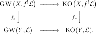
If we assume that
 $1/2 \in S$
and replace
$1/2 \in S$
and replace
 $\mathrm {GW}$
by
$\mathrm {GW}$
by
 $\mathrm {W}$
and
$\mathrm {W}$
and
 $\mathrm {KO}$
by
$\mathrm {KO}$
by
 $\mathrm {KW}$
, then maps
$\mathrm {KW}$
, then maps
 $\hat f_*$
can be defined and studied using the ideas from §2.2 (see also [Reference Calmès and Hornbostel22]). Levine and Raksit [Reference Levine and Raksit56] show that the (modified) diagram commutes, provided that X and Y are smooth over a common base with
$\hat f_*$
can be defined and studied using the ideas from §2.2 (see also [Reference Calmès and Hornbostel22]). Levine and Raksit [Reference Levine and Raksit56] show that the (modified) diagram commutes, provided that X and Y are smooth over a common base with
 $1/2 \in S$
.
$1/2 \in S$
.
If instead we assume that f is finite syntomic, then the analogous result is proved (for
 $\mathrm {GW} \to \mathrm {KO}$
and without
$\mathrm {GW} \to \mathrm {KO}$
and without
 $1/2 \in S$
) in Corollary A.4. This is the only case we shall use in the rest of this section. Recall the construction of the Scheja–Storch form
$1/2 \in S$
) in Corollary A.4. This is the only case we shall use in the rest of this section. Recall the construction of the Scheja–Storch form
 $\langle - \vert - \rangle ^{\mathrm {SS}}$
from Definition 2.20.
$\langle - \vert - \rangle ^{\mathrm {SS}}$
from Definition 2.20.
Corollary 8.2. Set
 $X \in {\mathrm {S}\mathrm {m}}_S$
, let
$X \in {\mathrm {S}\mathrm {m}}_S$
, let
 $V/X$
be a relatively oriented vector bundle with a very nondegenerate section
$V/X$
be a relatively oriented vector bundle with a very nondegenerate section
 $\sigma $
, and let Z be a clopen component of the zero scheme
$\sigma $
, and let Z be a clopen component of the zero scheme
 $Z(\sigma )$
. Suppose there exist coordinates
$Z(\sigma )$
. Suppose there exist coordinates
 $(\psi ,\varphi ,\sigma ^{\prime })$
around Z, as in Definition 2.28. Then
$(\psi ,\varphi ,\sigma ^{\prime })$
around Z, as in Definition 2.28. Then
 $$\begin{align*}\mathrm{ind}_Z(\sigma, \rho, \mathrm{KO}) = \left[\langle - \vert - \rangle^{\mathrm{SS}}(\varphi(U), \sigma^{\prime}, S)\right] \in \mathrm{KO}^0(S). \end{align*}$$
Proof. By Proposition 3.13, we may assume that
 $\psi = \operatorname {id}$
and so on; so in particular,
$\psi = \operatorname {id}$
and so on; so in particular,
 $X \subset \mathbb A^n_S$
. The result now follows from the identification of the transfers in Corollary A.4 (telling us that the index is given by the trace form from coherent duality) and Theorem 2.18 (identifying the coherent duality form with the Scheja–Storch form).
$X \subset \mathbb A^n_S$
. The result now follows from the identification of the transfers in Corollary A.4 (telling us that the index is given by the trace form from coherent duality) and Theorem 2.18 (identifying the coherent duality form with the Scheja–Storch form).
Corollary 8.3. Let S be regular semilocal scheme over a field k of characteristic
 $\ne 2$
.
$\ne 2$
.
-
(1) Let
$\varpi : S^{\prime } \to S$
be a finite syntomic morphism and
$\tau $
a trivialization of
$L_{\varpi } \in K(S^{\prime })$
. Then the associated endomorphism of the sphere spectrum over S is given under the isomorphism
of [Reference Bachmann and Hoyois10, Theorem 10.12] by the symmetric bilinear form
$$\begin{align*}\varpi_*\left(\mathcal O_{S^{\prime}}\right) \otimes \varpi_*\left(\mathcal O_{S^{\prime}}\right) \to \varpi_*\left(\mathcal O_{S^{\prime}}\right) \stackrel{\det(\tau)}{\simeq} \varpi_*\left(\omega_{S^{\prime}/S}\right) \xrightarrow{\eta_{\varpi}} \mathcal O_S. \end{align*}$$
-
(2) Let
$U \subset \mathbb A^n_S$
be open and define
$F: U \to \mathbb A^n$
to have an isolated zero along
$Z \subset U$
. Then


Proof. The proof of [Reference Bachmann and Hoyois10, Theorem 10.12] shows that the unit map
![]() induces the isomorphism
induces the isomorphism
![]() . (1) is an immediate consequence of Proposition 7.5, Lemma 4.6(1), and Corollary A.4. Via Corollary 7.4 and Theorem 2.18, (2) is a special case of (1). This concludes the proof.
. (1) is an immediate consequence of Proposition 7.5, Lemma 4.6(1), and Corollary A.4. Via Corollary 7.4 and Theorem 2.18, (2) is a special case of (1). This concludes the proof.
Corollary 8.4. Let X be essentially smooth over a field k of characteristic
 $\ne 2$
. Let
$\ne 2$
. Let
 $\varpi : X^{\prime } \to X$
be a finite syntomic morphism, and suppose an orientation
$\varpi : X^{\prime } \to X$
be a finite syntomic morphism, and suppose an orientation
 $\omega _{X^{\prime }/X} \stackrel {\rho }{\simeq } \mathcal L^{\otimes 2}$
. Consider the induced transfer
$\omega _{X^{\prime }/X} \stackrel {\rho }{\simeq } \mathcal L^{\otimes 2}$
. Consider the induced transfer
 $$\begin{align*}\varpi_*: \mathrm{H}\tilde{\mathbb{Z}}^0(X^{\prime}) \stackrel{\rho}{\simeq} \mathrm{H}\tilde{\mathbb{Z}}^0\left(X^{\prime}, \omega_{X^{\prime}/X}\right) \to \mathrm{H}\tilde{\mathbb{Z}}^0(X) \simeq \underline{GW}(X). \end{align*}$$
Then
 $\varpi _*(1)$
is given by the image in
$\varpi _*(1)$
is given by the image in
 $\underline {GW}(X)$
of the symmetric bilinear form on
$\underline {GW}(X)$
of the symmetric bilinear form on
 $$\begin{align*}\varpi_*(\mathcal L) \otimes \varpi_*(\mathcal L) \to \varpi_*\left(\mathcal L^{\otimes 2}\right) \stackrel{\rho}{\simeq} \varpi_*\left(\omega_{X^{\prime}/X}\right) \xrightarrow{\eta_{\varpi}} \mathcal O_X. \end{align*}$$
Proof. Using the unramifiedness of
 $\underline {GW}$
[Reference Morel60, Lemma 6.4.4], we may assume that X is the spectrum of a field. Then
$\underline {GW}$
[Reference Morel60, Lemma 6.4.4], we may assume that X is the spectrum of a field. Then
 $X^{\prime }$
is semilocal, so
$X^{\prime }$
is semilocal, so
 $\mathcal L \simeq \mathcal O$
and we obtain (up to choosing such an isomorphism)
$\mathcal L \simeq \mathcal O$
and we obtain (up to choosing such an isomorphism)
 $\omega _{X^{\prime }/X} \stackrel {\rho ^{\prime }}{\simeq } \mathcal O$
. Since
$\omega _{X^{\prime }/X} \stackrel {\rho ^{\prime }}{\simeq } \mathcal O$
. Since
 $L_{X^{\prime }/X}$
has constant rank (namely
$L_{X^{\prime }/X}$
has constant rank (namely
 $0$
), it follows from [Reference Bruns and Herzog17, Lemma 1.4.4] that
$0$
), it follows from [Reference Bruns and Herzog17, Lemma 1.4.4] that
 $L_{X^{\prime }/X} \simeq 0 \in K(X^{\prime })$
. The set of homotopy classes of such trivializations is given by
$L_{X^{\prime }/X} \simeq 0 \in K(X^{\prime })$
. The set of homotopy classes of such trivializations is given by
 $K_1(X^{\prime })$
, which maps surjectively (via the determinant) onto
$K_1(X^{\prime })$
, which maps surjectively (via the determinant) onto
 $\mathcal O^\times (X^{\prime })$
. It follows that there exists a trivialization
$\mathcal O^\times (X^{\prime })$
. It follows that there exists a trivialization
 $\tau : 0 \simeq L_{X^{\prime }/X} \in K(X^{\prime })$
such that
$\tau : 0 \simeq L_{X^{\prime }/X} \in K(X^{\prime })$
such that
 $\det (\tau ) = \rho ^{\prime }$
. Hence we have a commutative diagram
$\det (\tau ) = \rho ^{\prime }$
. Hence we have a commutative diagram
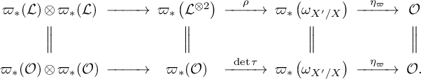
It follows from Corollary 8.3 that the bottom row is the form
 $\varpi _*(1)$
arising from the orientation
$\varpi _*(1)$
arising from the orientation
 $\rho $
; by what we just said, this is the same as the top row, which is the form we were supposed to obtain.
$\rho $
; by what we just said, this is the same as the top row, which is the form we were supposed to obtain.
This concludes the proof.
We also point out the following variant:
Corollary 8.5. Let
 $l/k$
be a finite extension of fields,
$l/k$
be a finite extension of fields,
 $1/2 \in k$
. Then Morel’s absolute transfer [Reference Morel61, §5.1]
$1/2 \in k$
. Then Morel’s absolute transfer [Reference Morel61, §5.1]
 $\mathrm {tr}_{l/k}: GW\left (l, \omega _{l/k}\right ) \to GW(k)$
is given as follows: Let
$\mathrm {tr}_{l/k}: GW\left (l, \omega _{l/k}\right ) \to GW(k)$
is given as follows: Let
 $\phi : V \otimes _l V \to l$
be an element of
$\phi : V \otimes _l V \to l$
be an element of
 $GW(l)$
,
$GW(l)$
,
 $\alpha \in \omega _{l/k}^\times $
. Then
$\alpha \in \omega _{l/k}^\times $
. Then
 $$\begin{align*}\mathrm{tr}_{l/k}(\phi \otimes \alpha) = \left[V \otimes_k V \to V \otimes_l V \xrightarrow{\phi} l \stackrel{\alpha}{\simeq} \omega_{l/k} \xrightarrow{\eta_{l/k}} k\right], \end{align*}$$
where
 $\eta _{l/k}: \omega _{l/k} \to k$
is the (k-linear) trace map of coherent duality (see §B.1).
$\eta _{l/k}: \omega _{l/k} \to k$
is the (k-linear) trace map of coherent duality (see §B.1).
Proof. This is immediate from [Reference Elmanto, Hoyois, Khan, Sosnilo and Yakerson31, Proposition 4.3.17] (telling us that Morel’s transfer coincides with the one from §4.2.4) and Corollary A.4.
Remark 8.6. Corollary 8.3(2) generalizes the main result of [Reference Kass and Wickelgren48], at least for fields of characteristic
 $\ne 2$
.
$\ne 2$
.
Remark 8.7. We expect that all of the results in this section extend to fields of characteristic
 $2$
as well. This should be automatic as soon as
$2$
as well. This should be automatic as soon as
 $\mathrm {KO}$
is shown to represent
$\mathrm {KO}$
is shown to represent
 $\mathrm {GW}$
in this situation (over regular bases, say).
$\mathrm {GW}$
in this situation (over regular bases, say).
Appendix A
$\mathrm {KO}$
via framed correspondences

In this section we will construct a strong orientation on
 $\mathrm {KO}$
and identify some of the transfers. We would like to thank M. Hoyois for communicating these results to us. For another approach to parts of the results in this section, see [Reference López-Ávila57].
$\mathrm {KO}$
and identify some of the transfers. We would like to thank M. Hoyois for communicating these results to us. For another approach to parts of the results in this section, see [Reference López-Ávila57].
We will make use of the technology of framed correspondences [Reference Elmanto, Hoyois, Khan, Sosnilo and Yakerson30]. We write
 $\mathrm {Corr}^{\mathrm {fr}}(S)$
for the symmetric monoidal
$\mathrm {Corr}^{\mathrm {fr}}(S)$
for the symmetric monoidal
 $\infty $
-category of smooth S-schemes and tangentially framed correspondences. Denote by
$\infty $
-category of smooth S-schemes and tangentially framed correspondences. Denote by
 $\mathrm {FSyn^{or}} \in \mathrm {CAlg}\left (\mathcal {P}_\Sigma \left (\mathrm {Corr}^{\mathrm {fr}}(S)\right )\right )$
the stack of finite syntomic schemes
$\mathrm {FSyn^{or}} \in \mathrm {CAlg}\left (\mathcal {P}_\Sigma \left (\mathrm {Corr}^{\mathrm {fr}}(S)\right )\right )$
the stack of finite syntomic schemes
 $Y/X$
together with a choice of trivialization
$Y/X$
together with a choice of trivialization
 $\det L_{Y/X} \simeq \mathcal O$
, with its standard structure of framed transfers. This is constructed in [Reference Elmanto, Hoyois, Khan, Sosnilo and Yakerson32, Example 3.3.4].
$\det L_{Y/X} \simeq \mathcal O$
, with its standard structure of framed transfers. This is constructed in [Reference Elmanto, Hoyois, Khan, Sosnilo and Yakerson32, Example 3.3.4].
Write
 $\mathrm {Bil} \in \mathrm {CAlg}(\mathcal {P}_\Sigma (\mathrm {S}\mathrm {ch}{}_S))$
for the presheaf sending X to the
$\mathrm {Bil} \in \mathrm {CAlg}(\mathcal {P}_\Sigma (\mathrm {S}\mathrm {ch}{}_S))$
for the presheaf sending X to the
 $1$
-groupoid of pairs
$1$
-groupoid of pairs
 $(V, \phi )$
with
$(V, \phi )$
with
 $V \to X$
a vector bundle and
$V \to X$
a vector bundle and
 $\phi : V \otimes V \to \mathcal O_X$
a nondegenerate, symmetric bilinear form. The commutative monoid structure is given by
$\phi : V \otimes V \to \mathcal O_X$
a nondegenerate, symmetric bilinear form. The commutative monoid structure is given by
 $\otimes $
. If
$\otimes $
. If
 $f: X \to Y$
is a finite syntomic morphism, then a choice of trivialization
$f: X \to Y$
is a finite syntomic morphism, then a choice of trivialization
 $\widetilde \det L_f \simeq \omega _f \simeq \mathcal O_X$
induces an additive map
$\widetilde \det L_f \simeq \omega _f \simeq \mathcal O_X$
induces an additive map
 $\hat f_*: \mathrm {Bil}^\simeq (X) \to \mathrm {Bil}^\simeq (Y)$
(see, e.g., §2.2).
$\hat f_*: \mathrm {Bil}^\simeq (X) \to \mathrm {Bil}^\simeq (Y)$
(see, e.g., §2.2).
Theorem A.1. There exists a lift
 $\mathrm {Bil} \in \mathrm {CAlg}\left (\mathcal {P}_\Sigma \left (\mathrm {Corr}^{\mathrm {fr}}(S)\right )\right )$
with the transfers given by maps of the form
$\mathrm {Bil} \in \mathrm {CAlg}\left (\mathcal {P}_\Sigma \left (\mathrm {Corr}^{\mathrm {fr}}(S)\right )\right )$
with the transfers given by maps of the form
 $\hat f_*$
, together with a morphism
$\hat f_*$
, together with a morphism
 $\mathrm {FSyn^{or}} \to \mathrm {Bil} \in \mathrm {CAlg}\left (\mathcal {P}_\Sigma \left (\mathrm {Corr}^{\mathrm {fr}}(S)\right )\right )$
.
$\mathrm {FSyn^{or}} \to \mathrm {Bil} \in \mathrm {CAlg}\left (\mathcal {P}_\Sigma \left (\mathrm {Corr}^{\mathrm {fr}}(S)\right )\right )$
.
The morphism
 $\mathrm {FSyn^{or}} \to \mathrm {Bil}$
is informally described as follows: a pair
$\mathrm {FSyn^{or}} \to \mathrm {Bil}$
is informally described as follows: a pair
 $(f: X \to Y \text{ finite}\text{syntomic},\ \omega _f \simeq \mathcal O)$
is sent to
$(f: X \to Y \text{ finite}\text{syntomic},\ \omega _f \simeq \mathcal O)$
is sent to
 $f_*(\mathcal O)$
, where
$f_*(\mathcal O)$
, where
 $\mathcal O \in \mathrm {Bil}(X)$
denotes the vector bundle
$\mathcal O \in \mathrm {Bil}(X)$
denotes the vector bundle
 $\mathcal O_X$
with its canonical symmetric bilinear pairing
$\mathcal O_X$
with its canonical symmetric bilinear pairing
 $\mathcal O_X \otimes \mathcal O_X \to \mathcal O_X$
.
$\mathcal O_X \otimes \mathcal O_X \to \mathcal O_X$
.
Proof. Denote by
 $K^\circ \in \mathcal {P}_\Sigma ({\mathrm {S}\mathrm {m}}_S)$
the rank
$K^\circ \in \mathcal {P}_\Sigma ({\mathrm {S}\mathrm {m}}_S)$
the rank
 $0$
part of the K-theory presheaf and by
$0$
part of the K-theory presheaf and by
 $\mathrm {Corr}^{\mathrm {fr}}\left (({\mathrm {S}\mathrm {m}}_S)_{/K^\circ }\right )$
the subcategory of the category constructed in [Reference Elmanto, Hoyois, Khan, Sosnilo and Yakerson32, §B] on objects
$\mathrm {Corr}^{\mathrm {fr}}\left (({\mathrm {S}\mathrm {m}}_S)_{/K^\circ }\right )$
the subcategory of the category constructed in [Reference Elmanto, Hoyois, Khan, Sosnilo and Yakerson32, §B] on objects
 $(X, \xi )$
with
$(X, \xi )$
with
 $X \in {\mathrm {S}\mathrm {m}}_S$
,
$X \in {\mathrm {S}\mathrm {m}}_S$
,
 $\xi $
of rank
$\xi $
of rank
 $0$
, and morphisms those spans whose left leg is finite syntomic. There are symmetric monoidal functors
$0$
, and morphisms those spans whose left leg is finite syntomic. There are symmetric monoidal functors
 $\gamma : ({\mathrm {S}\mathrm {m}}_S)_{/K^\circ } \to \mathrm {Corr}^{\mathrm {fr}}\left (({\mathrm {S}\mathrm {m}}_S)_{/K^\circ }\right )$
and
$\gamma : ({\mathrm {S}\mathrm {m}}_S)_{/K^\circ } \to \mathrm {Corr}^{\mathrm {fr}}\left (({\mathrm {S}\mathrm {m}}_S)_{/K^\circ }\right )$
and
 $\delta : \mathrm {Corr}^{\mathrm {fr}}(S) \to \mathrm {Corr}^{\mathrm {fr}}\left (({\mathrm {S}\mathrm {m}}_S)_{/K^\circ }\right )$
.
$\delta : \mathrm {Corr}^{\mathrm {fr}}(S) \to \mathrm {Corr}^{\mathrm {fr}}\left (({\mathrm {S}\mathrm {m}}_S)_{/K^\circ }\right )$
.
We first lift
 $\mathrm {Bil}$
to
$\mathrm {Bil}$
to
 $\mathcal {P}_\Sigma \left (\mathrm {Corr}^{\mathrm {fr}}(({\mathrm {S}\mathrm {m}}_S)_{/K^\circ })\right )$
; we let
$\mathcal {P}_\Sigma \left (\mathrm {Corr}^{\mathrm {fr}}(({\mathrm {S}\mathrm {m}}_S)_{/K^\circ })\right )$
; we let
 $\mathrm {Bil}(X, \xi )$
be the
$\mathrm {Bil}(X, \xi )$
be the
 $1$
-groupoid of vector bundles with a symmetric bilinear form for the duality
$1$
-groupoid of vector bundles with a symmetric bilinear form for the duality
 $\underline {\operatorname {Hom}}(\mathord -, \det \xi )$
. Since
$\underline {\operatorname {Hom}}(\mathord -, \det \xi )$
. Since
 $\mathrm {Bil}$
is
$\mathrm {Bil}$
is
 $1$
-truncated, we only need to specify a finite number of coherence homotopies, so this can be done by hand. Since
$1$
-truncated, we only need to specify a finite number of coherence homotopies, so this can be done by hand. Since
 $\delta $
is symmetric monoidal,
$\delta $
is symmetric monoidal,
 $\delta ^*$
is lax symmetric monoidal, and hence
$\delta ^*$
is lax symmetric monoidal, and hence
 $\delta ^*(\mathrm {Bil})$
produces the desired lift.
$\delta ^*(\mathrm {Bil})$
produces the desired lift.
Let
 $K^{\prime } \to K^\circ $
denote the fiber of the determinant map; in other words, this is the rank
$K^{\prime } \to K^\circ $
denote the fiber of the determinant map; in other words, this is the rank
 $0$
part of
$0$
part of
 $K^{\mathrm {SL}}$
. This defines an object of
$K^{\mathrm {SL}}$
. This defines an object of
 $\mathrm {CAlg}\left (\mathcal {P}_\Sigma ({\mathrm {S}\mathrm {m}}_S)_{/K^\circ }\right ) \simeq \mathrm {CAlg}\left (\mathcal {P}_\Sigma \left (({\mathrm {S}\mathrm {m}}_S)_{/K^\circ }\right )\right )$
and
$\mathrm {CAlg}\left (\mathcal {P}_\Sigma ({\mathrm {S}\mathrm {m}}_S)_{/K^\circ }\right ) \simeq \mathrm {CAlg}\left (\mathcal {P}_\Sigma \left (({\mathrm {S}\mathrm {m}}_S)_{/K^\circ }\right )\right )$
and
 $\gamma K^{\prime } \simeq \mathrm {FSyn^{or}}$
[Reference Elmanto, Hoyois, Khan, Sosnilo and Yakerson32, Example 3.3.4 and after Example 3.3.6]. To conclude the proof, it thus suffices to construct a map
$\gamma K^{\prime } \simeq \mathrm {FSyn^{or}}$
[Reference Elmanto, Hoyois, Khan, Sosnilo and Yakerson32, Example 3.3.4 and after Example 3.3.6]. To conclude the proof, it thus suffices to construct a map
 $K^{\prime } \to \gamma ^*(\mathrm {Bil}) \in \mathrm {CAlg}\left (\mathcal {P}_\Sigma ({\mathrm {S}\mathrm {m}}_S)_{/K^\circ }\right )$
. Again, this needs only a finite number of coherences; the desired map sends
$K^{\prime } \to \gamma ^*(\mathrm {Bil}) \in \mathrm {CAlg}\left (\mathcal {P}_\Sigma ({\mathrm {S}\mathrm {m}}_S)_{/K^\circ }\right )$
. Again, this needs only a finite number of coherences; the desired map sends
 $(\xi , \phi )$
with
$(\xi , \phi )$
with
 $\xi \in K^\circ (X)$
and
$\xi \in K^\circ (X)$
and
 $\phi : \det (\xi ) \simeq \mathcal O_X$
to
$\phi : \det (\xi ) \simeq \mathcal O_X$
to
 $(\mathcal O, \phi ^{\prime })$
, where
$(\mathcal O, \phi ^{\prime })$
, where
 $\phi ^{\prime }: \mathcal O \otimes \mathcal O \simeq \mathcal O \stackrel {\phi }{\simeq } \det \xi $
.
$\phi ^{\prime }: \mathcal O \otimes \mathcal O \simeq \mathcal O \stackrel {\phi }{\simeq } \det \xi $
.
Since group completion and Zariski localization commute with the forgetful functor
 $\mathcal {P}_\Sigma \left (\mathrm {Corr}^{\mathrm {fr}}_S\right ) \to \mathrm {CMon}(\mathcal {P}_\Sigma ({\mathrm {S}\mathrm {m}}_S)) \to \mathcal {P}_\Sigma ({\mathrm {S}\mathrm {m}}_S)$
[Reference Elmanto, Hoyois, Khan, Sosnilo and Yakerson30, Proposition 3.2.14], we deduce that
$\mathcal {P}_\Sigma \left (\mathrm {Corr}^{\mathrm {fr}}_S\right ) \to \mathrm {CMon}(\mathcal {P}_\Sigma ({\mathrm {S}\mathrm {m}}_S)) \to \mathcal {P}_\Sigma ({\mathrm {S}\mathrm {m}}_S)$
[Reference Elmanto, Hoyois, Khan, Sosnilo and Yakerson30, Proposition 3.2.14], we deduce that
 $(L_{\mathrm {Zar}} \mathrm {Bil}^{gp})(X) \simeq \mathrm {KO}(X)$
[Reference Hornbostel42, Definitions 1.5 and 2.2]; we denote this presheaf by
$(L_{\mathrm {Zar}} \mathrm {Bil}^{gp})(X) \simeq \mathrm {KO}(X)$
[Reference Hornbostel42, Definitions 1.5 and 2.2]; we denote this presheaf by
 $\mathrm {GW}$
. There is thus a canonical Bott element
$\mathrm {GW}$
. There is thus a canonical Bott element
 $\beta \in \left [T^4, \mathrm {GW}\right ]$
.
$\beta \in \left [T^4, \mathrm {GW}\right ]$
.
Proposition A.2. There is a canonical equivalence
 $\left (\Sigma ^\infty _{\mathrm {fr}} \mathrm {GW}\right )\left [\beta ^{-1}\right ] \simeq \mathrm {KO}$
, at least if
$\left (\Sigma ^\infty _{\mathrm {fr}} \mathrm {GW}\right )\left [\beta ^{-1}\right ] \simeq \mathrm {KO}$
, at least if
 $1/2 \in S$
.
$1/2 \in S$
.
Proof. The spectrum
 $\left (\Sigma ^\infty _{\mathrm {fr}} \mathrm {GW}\right )\left [\beta ^{-1}\right ] \in \mathcal {SH}^{\mathrm {fr}}(S)$
can be modeled by the framed
$\left (\Sigma ^\infty _{\mathrm {fr}} \mathrm {GW}\right )\left [\beta ^{-1}\right ] \in \mathcal {SH}^{\mathrm {fr}}(S)$
can be modeled by the framed
 $T^4$
-prespectrum
$T^4$
-prespectrum
 $(\mathrm {GW}, \mathrm {GW}, \dots )$
with the bonding maps given by multiplication by
$(\mathrm {GW}, \mathrm {GW}, \dots )$
with the bonding maps given by multiplication by
 $\beta $
. Under the equivalence
$\beta $
. Under the equivalence
 $\mathcal {SH}^{\mathrm {fr}}(S) \simeq \mathcal {SH}(S)$
[Reference Hoyois45], this corresponds to the same prespectrum with transfers forgotten. This is
$\mathcal {SH}^{\mathrm {fr}}(S) \simeq \mathcal {SH}(S)$
[Reference Hoyois45], this corresponds to the same prespectrum with transfers forgotten. This is
 $\mathrm {KO}$
by definition.
$\mathrm {KO}$
by definition.
In particular, we have constructed an
 $\mathcal E_\infty $
-structure on
$\mathcal E_\infty $
-structure on
 $\mathrm {KO}$
.
$\mathrm {KO}$
.
Corollary A.3. There is a morphism
 $\mathrm {MSL} \to \mathrm {KO} \in \mathrm {CAlg}(\mathcal {SH}(S))$
, at least if
$\mathrm {MSL} \to \mathrm {KO} \in \mathrm {CAlg}(\mathcal {SH}(S))$
, at least if
 $1/2 \in S$
.
$1/2 \in S$
.
Proof. Take the morphism
 $\Sigma ^\infty _{\mathrm {fr}} \mathrm {FSyn^{or}} \to \Sigma ^\infty _{\mathrm {fr}} \mathrm {Bil} \to \Sigma ^\infty _{\mathrm {fr}} \mathrm {GW} \to \mathrm {KO}$
and use the fact that
$\Sigma ^\infty _{\mathrm {fr}} \mathrm {FSyn^{or}} \to \Sigma ^\infty _{\mathrm {fr}} \mathrm {Bil} \to \Sigma ^\infty _{\mathrm {fr}} \mathrm {GW} \to \mathrm {KO}$
and use the fact that
 $\Sigma ^\infty _{\mathrm {fr}} \mathrm {FSyn^{or}} \simeq \mathrm {MSL}$
[Reference Elmanto, Hoyois, Khan, Sosnilo and Yakerson32, Theorem 3.4.3(i)].
$\Sigma ^\infty _{\mathrm {fr}} \mathrm {FSyn^{or}} \simeq \mathrm {MSL}$
[Reference Elmanto, Hoyois, Khan, Sosnilo and Yakerson32, Theorem 3.4.3(i)].
Corollary A.4. Let
 $f: Z \to S$
be a finite syntomic morphism, with
$f: Z \to S$
be a finite syntomic morphism, with
 $1/2 \in S$
,
$1/2 \in S$
,
 $\tau : L_{Z/S} \simeq 0 \in K(Z)$
a trivialization, and
$\tau : L_{Z/S} \simeq 0 \in K(Z)$
a trivialization, and
 $\phi : V \otimes V \to \mathcal O_Z$
be a nondegenerate, symmetric bilinear form (defining an element
$\phi : V \otimes V \to \mathcal O_Z$
be a nondegenerate, symmetric bilinear form (defining an element
 $[\phi ] \in \mathrm {KO}^0(Z)$
). Then
$[\phi ] \in \mathrm {KO}^0(Z)$
). Then
 $$\begin{align*}\left[\hat f_*(\phi)\right] = f_*([\phi]) \in \mathrm{KO}^0(S). \end{align*}$$
Here
 $f_*$
denotes the transfer arising from the six-functors formalism, and
$f_*$
denotes the transfer arising from the six-functors formalism, and
 $\hat f_*$
denotes the transfer constructed before using coherent duality.
$\hat f_*$
denotes the transfer constructed before using coherent duality.
Proof. We first give a simplified proof assuming that S is affine. Denote by
 $\mathrm {KO}^{\mathrm {fr}} \in \mathcal {SH}^{\mathrm {fr}}(S)$
a lift of
$\mathrm {KO}^{\mathrm {fr}} \in \mathcal {SH}^{\mathrm {fr}}(S)$
a lift of
 $\mathrm {KO}$
. By [Reference Elmanto, Hoyois, Khan, Sosnilo and Yakerson31, Theorem 3.3.10], for any morphism
$\mathrm {KO}$
. By [Reference Elmanto, Hoyois, Khan, Sosnilo and Yakerson31, Theorem 3.3.10], for any morphism
 $p: Z \to Y$
with
$p: Z \to Y$
with
 $Y \in {\mathrm {S}\mathrm {m}}_S$
and a form
$Y \in {\mathrm {S}\mathrm {m}}_S$
and a form
 $\psi $
on Y, the six-functors transfer of
$\psi $
on Y, the six-functors transfer of
 $p^*([\psi ])$
along f coincides with the framed transfer of
$p^*([\psi ])$
along f coincides with the framed transfer of
 $[\psi ]$
along the correspondence
$[\psi ]$
along the correspondence
 $S \xleftarrow {\tau } Z \to Y$
. By Proposition A.2, we can take
$S \xleftarrow {\tau } Z \to Y$
. By Proposition A.2, we can take
 $\mathrm {KO}^{\mathrm {fr}} = \Sigma ^\infty _{\mathrm {fr}} \mathrm {GW}\left [\beta ^{-1}\right ]$
; it follows that there is a map
$\mathrm {KO}^{\mathrm {fr}} = \Sigma ^\infty _{\mathrm {fr}} \mathrm {GW}\left [\beta ^{-1}\right ]$
; it follows that there is a map
 $\mathrm {Bil} \to \Omega ^\infty _{\mathrm {fr}} \mathrm {KO}^{\mathrm {fr}} \in \mathcal {P}_\Sigma \left (\mathrm {Corr}^{\mathrm {fr}}\right )$
. We thus deduce that
$\mathrm {Bil} \to \Omega ^\infty _{\mathrm {fr}} \mathrm {KO}^{\mathrm {fr}} \in \mathcal {P}_\Sigma \left (\mathrm {Corr}^{\mathrm {fr}}\right )$
. We thus deduce that
 $$\begin{align*}\hat f_*(p^* \psi) = f_*(p^*[\psi]) \in \mathrm{KO}^0(S). \end{align*}$$
The result would follow if there exist p,
 $\psi $
with
$\psi $
with
 $p^* \psi = \phi $
. Under our simplifying assumption that S is affine, this is always the case [Reference Elmanto, Hoyois, Khan, Sosnilo and Yakerson32, Proposition A.0.4 and Example A.0.6(5)].
$p^* \psi = \phi $
. Under our simplifying assumption that S is affine, this is always the case [Reference Elmanto, Hoyois, Khan, Sosnilo and Yakerson32, Proposition A.0.4 and Example A.0.6(5)].
To deal with the general case, we begin with some constructions. Given
 $F \in \mathcal {P}({\mathrm {S}\mathrm {m}}_S)$
, denote by
$F \in \mathcal {P}({\mathrm {S}\mathrm {m}}_S)$
, denote by
 $f^* F \in \mathcal {P}({\mathrm {S}\mathrm {m}}_Z)$
the left Kan extension. If F comes from a presheaf with framed transfers, then the transfers along (base changes of) f assemble to a map
$f^* F \in \mathcal {P}({\mathrm {S}\mathrm {m}}_Z)$
the left Kan extension. If F comes from a presheaf with framed transfers, then the transfers along (base changes of) f assemble to a map
 $f_*f^* F \to F$
. Given
$f_*f^* F \to F$
. Given
 $E \in \mathcal {SH}(S)$
, we obtain
$E \in \mathcal {SH}(S)$
, we obtain
 $\Omega ^\infty E \in \mathcal {P}({\mathrm {S}\mathrm {m}}_S)$
and can apply this construction. On the other hand, there is a map
$\Omega ^\infty E \in \mathcal {P}({\mathrm {S}\mathrm {m}}_S)$
and can apply this construction. On the other hand, there is a map
 $f_* \Omega ^\infty f^* E \to \Omega ^\infty E$
coming from the six-functors transfer as well as a map
$f_* \Omega ^\infty f^* E \to \Omega ^\infty E$
coming from the six-functors transfer as well as a map
 $f^* \Omega ^\infty E \to \Omega ^\infty f^* E$
, and [Reference Elmanto, Hoyois, Khan, Sosnilo and Yakerson31, Theorem 3.3.10] implies that the following diagram commutes
$f^* \Omega ^\infty E \to \Omega ^\infty f^* E$
, and [Reference Elmanto, Hoyois, Khan, Sosnilo and Yakerson31, Theorem 3.3.10] implies that the following diagram commutes
Now we continue with the proof. We have a commutative diagram
where
 $\mathrm {Bil}_T \in \mathcal {P}({\mathrm {S}\mathrm {m}}_T)$
denotes the stack of symmetric bilinear forms, the map
$\mathrm {Bil}_T \in \mathcal {P}({\mathrm {S}\mathrm {m}}_T)$
denotes the stack of symmetric bilinear forms, the map
 $f_*f^* \mathrm {Bil}_S \to \mathrm {Bil}_S$
comes from the construction with
$f_*f^* \mathrm {Bil}_S \to \mathrm {Bil}_S$
comes from the construction with
 $F = \mathrm {Bil}_S$
, the map
$F = \mathrm {Bil}_S$
, the map
 $f_* \mathrm {Bil}_Z \to \mathrm {Bil}_S$
is the transfer
$f_* \mathrm {Bil}_Z \to \mathrm {Bil}_S$
is the transfer
 $\hat f_*$
, and commutativity holds by construction. Applying the construction with
$\hat f_*$
, and commutativity holds by construction. Applying the construction with
 $E = \mathrm {KO}$
and using its naturality in F, we obtain all in all the following commutative diagram:
$E = \mathrm {KO}$
and using its naturality in F, we obtain all in all the following commutative diagram:
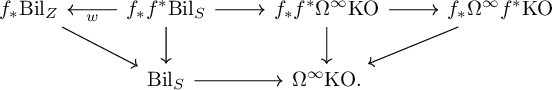
It follows from [Reference Elmanto, Hoyois, Khan, Sosnilo and Yakerson32, Proposition A.0.4 and Example A.0.6(5)] that
 $f^* \mathrm {Bil}_S \to \mathrm {Bil}_Z$
is a Zariski equivalence, and hence the map labeled w is a Nisnevich equivalence (f being finite). Since
$f^* \mathrm {Bil}_S \to \mathrm {Bil}_Z$
is a Zariski equivalence, and hence the map labeled w is a Nisnevich equivalence (f being finite). Since
 $f_* \Omega ^\infty f^* \mathrm {KO}$
and
$f_* \Omega ^\infty f^* \mathrm {KO}$
and
 $\Omega ^\infty \mathrm {KO}$
are Nisnevich local, we may invert w to obtain the following commutative diagram:
$\Omega ^\infty \mathrm {KO}$
are Nisnevich local, we may invert w to obtain the following commutative diagram:
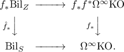
The result follows.
Remark A.5. If
 $1/2 \not \in S$
, then we could define
$1/2 \not \in S$
, then we could define
 $\mathrm {KO}$
as
$\mathrm {KO}$
as
 $\left (\Sigma ^\infty _{\mathrm {fr}} \mathrm {GW}\right )\left [\beta ^{-1}\right ]$
. Then Corollaries A.3 and A.4 (as well as Proposition A.2) remain true. The problem is that we no longer know what theory
$\left (\Sigma ^\infty _{\mathrm {fr}} \mathrm {GW}\right )\left [\beta ^{-1}\right ]$
. Then Corollaries A.3 and A.4 (as well as Proposition A.2) remain true. The problem is that we no longer know what theory
 $\mathrm {KO}$
represents.
$\mathrm {KO}$
represents.
Appendix B Miscellaneous
We collect some results which we believe are well known, but for which we could not find convenient references.
B.1 Cotangent complexes and dualizing complexes
For any morphism of schemes
 $f: X \to Y$
, there is the cotangent complex
$f: X \to Y$
, there is the cotangent complex
 $L_f \in D(X)$
(see, e.g., [73, Tag 08P5]). If f is lci, then
$L_f \in D(X)$
(see, e.g., [73, Tag 08P5]). If f is lci, then
 $L_f$
is perfect [73, Tag 08SH] and hence defines a point
$L_f$
is perfect [73, Tag 08SH] and hence defines a point
 $L_f \in K(X)$
. Consequently, in this case we can make sense of the graded determinant
$L_f \in K(X)$
. Consequently, in this case we can make sense of the graded determinant
 $\widetilde \det L_f \in \mathrm {Pic}(D(X))$
; this is (locally) a shift of a line bundle.
$\widetilde \det L_f \in \mathrm {Pic}(D(X))$
; this is (locally) a shift of a line bundle.
Proposition B.1. Let
 $f: X \to Y$
be lci. Then there is a canonical isomorphism
$f: X \to Y$
be lci. Then there is a canonical isomorphism
 $f^! \mathcal O_Y \simeq \widetilde \det L_f$
.
$f^! \mathcal O_Y \simeq \widetilde \det L_f$
.
Recall that by our conventions, X and Y are separated and of finite type over some Noetherian scheme S; in particular, they are themselves Noetherian. We strongly believe that these assumptions are immaterial.
Proof of Proposition B.1. Both sides are compatible with passage to open subschemes of X. Locally on X, f factors as a regular immersion followed by a smooth morphism, say
 $f=pi$
. For either a regular immersion or a smooth morphism g, we have isomorphisms
$f=pi$
. For either a regular immersion or a smooth morphism g, we have isomorphisms
 $$ \begin{align} g^! \mathcal O_Y \simeq \widetilde\det L_g, \end{align} $$
as desired [Reference Hartshorne40, Definition III.2, Proposition 7.2]. For composable lci morphisms
 $p, i$
, we have
$p, i$
, we have
 $$ \begin{align} (pi)^!(\mathcal O) \simeq i^*p^!(\mathcal O) \otimes i^!(\mathcal O).\end{align} $$
Similarly we have a canonical cofiber sequence
 $i^* L_p \to L_{pi} \to L_i$
, and hence
$i^* L_p \to L_{pi} \to L_i$
, and hence
 $$ \begin{align} \widetilde \det L_{pi} \simeq i^* \widetilde \det L_p \otimes \widetilde \det L_i.\end{align} $$
Combining formula (18), (19), and (20), we thus obtain an isomorphism
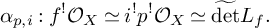 $$\begin{align*}\alpha_{p,i}: f^! \mathcal O_X \simeq i^!p^! \mathcal O_X \simeq \widetilde \det L_f. \end{align*}$$
We have thus shown that
 $f^! \mathcal O_Y$
is locally isomorphic to
$f^! \mathcal O_Y$
is locally isomorphic to
 $\widetilde \det L_f$
(via
$\widetilde \det L_f$
(via
 $\alpha _{p,i}$
), and hence that
$\alpha _{p,i}$
), and hence that
 $A := f^! \mathcal O_Y \otimes \left (\widetilde \det L_f\right )^{-1}$
is an
$A := f^! \mathcal O_Y \otimes \left (\widetilde \det L_f\right )^{-1}$
is an
 $\mathcal O_X$
-module concentrated in degree
$\mathcal O_X$
-module concentrated in degree
 $0$
. Exhibiting an isomorphism as claimed is the same as exhibiting
$0$
. Exhibiting an isomorphism as claimed is the same as exhibiting
 $A \simeq \mathcal O_X$
, or equivalently a section
$A \simeq \mathcal O_X$
, or equivalently a section
 $a \in \Gamma (X, A)$
which locally on X corresponds to an isomorphism. Since A is
$a \in \Gamma (X, A)$
which locally on X corresponds to an isomorphism. Since A is
 $0$
-truncated, we may construct a locally. In other words, we need to exhibit a cover
$0$
-truncated, we may construct a locally. In other words, we need to exhibit a cover
 $\{U_n\}_n$
of X and isomorphisms
$\{U_n\}_n$
of X and isomorphisms
 $\alpha _n: f^! \mathcal O_Y\rvert _{U_n} \simeq \widetilde \det L_f\rvert _{U_n}$
such that on
$\alpha _n: f^! \mathcal O_Y\rvert _{U_n} \simeq \widetilde \det L_f\rvert _{U_n}$
such that on
 $U_n \cap U_m$
we have
$U_n \cap U_m$
we have
 $\alpha _n \simeq \alpha _m$
. Hence, since we are claiming to exhibit a canonical isomorphism, we may do so locally on X. We may thus assume that f factors as
$\alpha _n \simeq \alpha _m$
. Hence, since we are claiming to exhibit a canonical isomorphism, we may do so locally on X. We may thus assume that f factors as
 $pi$
, for a smooth morphism
$pi$
, for a smooth morphism
 $p: V \to Y$
and a regular immersion
$p: V \to Y$
and a regular immersion
 $i: X \to V$
. We have already found an isomorphism in this situation, namely
$i: X \to V$
. We have already found an isomorphism in this situation, namely
 $\alpha _{p,i}$
. What remains is to show that this isomorphism is independent of the choice of factorization
$\alpha _{p,i}$
. What remains is to show that this isomorphism is independent of the choice of factorization
 $f = pi$
.
$f = pi$
.
Thus let
 $i^{\prime }: X \to V^{\prime }$
and
$i^{\prime }: X \to V^{\prime }$
and
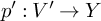 $p^{\prime }: V^{\prime } \to Y$
be another such factorization. We need to show that
$p^{\prime }: V^{\prime } \to Y$
be another such factorization. We need to show that
 $\alpha _{p,i} = \alpha _{p^{\prime },i^{\prime }}$
. By considering
$\alpha _{p,i} = \alpha _{p^{\prime },i^{\prime }}$
. By considering
 $V^{\prime } \times _Y V$
, we may assume a commutative diagram
$V^{\prime } \times _Y V$
, we may assume a commutative diagram
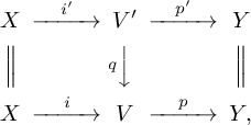
where q is smooth. If in formula (20) both f and g are smooth, then the isomorphism arises from the first fundamental exact sequence of K
 $\ddot {a}$
hler differentials [Reference Hartshorne40, Proposition III.2.2], and hence is the same as isomorphism (19). It follows that we may assume that
$\ddot {a}$
hler differentials [Reference Hartshorne40, Proposition III.2.2], and hence is the same as isomorphism (19). It follows that we may assume that
 $p=\operatorname {id}$
. The isomorphism
$p=\operatorname {id}$
. The isomorphism
 $i^{\prime !} q^! \simeq i^!$
is explained in [Reference Hartshorne40, Proposition III.8.2] and reduces via formal considerations (that apply in the same way to
$i^{\prime !} q^! \simeq i^!$
is explained in [Reference Hartshorne40, Proposition III.8.2] and reduces via formal considerations (that apply in the same way to
 $\widetilde \det L_{\mathord -}$
) to the case of a smooth morphism with a section.
$\widetilde \det L_{\mathord -}$
) to the case of a smooth morphism with a section.
We are thus reduced to the following problem: Let
 $p: V \to X$
be smooth and
$p: V \to X$
be smooth and
 $i: X \to V$
a regular immersion which is a section of p. The coherent duality formalism provides us with an isomorphism
$i: X \to V$
a regular immersion which is a section of p. The coherent duality formalism provides us with an isomorphism
 $\omega _{X/V} \otimes i^* \omega _{V/X} \simeq \mathcal O_X$
; we need to check that this is the same as the isomorphism
$\omega _{X/V} \otimes i^* \omega _{V/X} \simeq \mathcal O_X$
; we need to check that this is the same as the isomorphism
 $\det L_i \otimes i^* \det L_p \simeq \det L_{\operatorname {id}} = \mathcal O_X$
coming from formula (20). By [Reference Hartshorne40, Lemma III.8.1, Definition III.1.5], the first isomorphism arises from the second fundamental exact sequence of K
$\det L_i \otimes i^* \det L_p \simeq \det L_{\operatorname {id}} = \mathcal O_X$
coming from formula (20). By [Reference Hartshorne40, Lemma III.8.1, Definition III.1.5], the first isomorphism arises from the second fundamental exact sequence of K
 $\ddot {a}$
hler differentials. This is the same as the second isomorphism.
$\ddot {a}$
hler differentials. This is the same as the second isomorphism.
This concludes the proof.□
B.2 Grothendieck–Witt rings and Witt rings
Let R be a commutative ring. A symmetric space over R means a finitely generated projective R-module M together with a nondegenerate, symmetric bilinear form
 $\varphi : M \times M \to R$
. The Grothendieck group on the semiring of isomorphism classes of symmetric spaces over R (with operations given by the direct sum and tensor product) is denoted
$\varphi : M \times M \to R$
. The Grothendieck group on the semiring of isomorphism classes of symmetric spaces over R (with operations given by the direct sum and tensor product) is denoted
 $\mathrm {GW}(R)$
and called the Grothendieck–Witt ring of R. A symmetric space
$\mathrm {GW}(R)$
and called the Grothendieck–Witt ring of R. A symmetric space
 $(M, \varphi )$
is called metabolic if there exists a summand
$(M, \varphi )$
is called metabolic if there exists a summand
 $N \subset M$
with
$N \subset M$
with
 $N = N^\perp $
. The quotient of
$N = N^\perp $
. The quotient of
 $\mathrm {GW}(R)$
by the subgroup (which is an ideal) generated by metabolic spaces is denoted
$\mathrm {GW}(R)$
by the subgroup (which is an ideal) generated by metabolic spaces is denoted
 $\mathrm {W}(R)$
and called the Witt ring of R.
$\mathrm {W}(R)$
and called the Witt ring of R.
Lemma B.2. Let R be a commutative ring and
 $(M, \varphi )$
a symmetric space. The following are equivalent:
$(M, \varphi )$
a symmetric space. The following are equivalent:
-
(1) M is metabolic.
-
(2) M contains an isotropic subspace of half rank: there exists a summand
$N \subset M$
such that
$\dim M = 2 \dim N$
and
$\varphi \rvert _N = 0$
.


Now suppose that all finitely generated projective R-modules are free of constant rank–for example, R a local ring. In this case the image of M in
 $\mathrm {GW}(R)$
is given by
$\mathrm {GW}(R)$
is given by
 $nh$
, where
$nh$
, where
 $\dim M = 2n$
and h denotes the hyperbolic plane, corresponding to the matrix
$\dim M = 2n$
and h denotes the hyperbolic plane, corresponding to the matrix
 $\begin {pmatrix} 0 & 1 \\ 1 & 0 \end {pmatrix}$
, which also satisfies
$\begin {pmatrix} 0 & 1 \\ 1 & 0 \end {pmatrix}$
, which also satisfies
 $h = 1 + \langle -1 \rangle \in \mathrm {GW}(R)$
. Moreover we have a pullback square
$h = 1 + \langle -1 \rangle \in \mathrm {GW}(R)$
. Moreover we have a pullback square
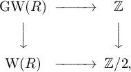
where the horizontal maps are given by rank. In particular
 $\mathrm {GW}(R) \to \mathrm {W}(R) \times \mathbb {Z}$
is injective.
$\mathrm {GW}(R) \to \mathrm {W}(R) \times \mathbb {Z}$
is injective.
Proof. The equivalence of (1) and (2) is [Reference Knebusch51, Corollary I.3.2]. The fact that the image in
 $\mathrm {GW}(R)$
is given by
$\mathrm {GW}(R)$
is given by
 $nh$
follows from [Reference Knebusch51, Proposition I.3.2 and Corollary I.3.1].
$nh$
follows from [Reference Knebusch51, Proposition I.3.2 and Corollary I.3.1].
Consider the symmetric space
 $M=\langle 1 \rangle \oplus h$
. Thus
$M=\langle 1 \rangle \oplus h$
. Thus
 $M \simeq R^3$
has basis
$M \simeq R^3$
has basis
 $e_1, e_2, e_3$
with
$e_1, e_2, e_3$
with
 $\langle e_1,e_1 \rangle = 1$
,
$\langle e_1,e_1 \rangle = 1$
,
 $\langle e_1, e_2 \rangle = 0$
, and so on. Direct computation shows that
$\langle e_1, e_2 \rangle = 0$
, and so on. Direct computation shows that
 $f_1 = e_1 + e_2$
,
$f_1 = e_1 + e_2$
,
 $f_2 = e_1 - e_3$
,
$f_2 = e_1 - e_3$
,
 $f_3 = e_3 - e_1 - e_2$
are an orthogonal basis exhibiting
$f_3 = e_3 - e_1 - e_2$
are an orthogonal basis exhibiting
 $M \simeq \langle 1 \rangle \oplus \langle 1 \rangle \oplus \langle -1 \rangle $
. Thus
$M \simeq \langle 1 \rangle \oplus \langle 1 \rangle \oplus \langle -1 \rangle $
. Thus
 $h = 1 + \langle -1 \rangle \in \mathrm {GW}(R)$
, as claimed.
$h = 1 + \langle -1 \rangle \in \mathrm {GW}(R)$
, as claimed.
We have
 $\mathrm {W}(R) = \mathrm {GW}(R)/J$
, where the ideal J is generated by metabolic spaces. By the previous assertion,
$\mathrm {W}(R) = \mathrm {GW}(R)/J$
, where the ideal J is generated by metabolic spaces. By the previous assertion,
 $J=\mathbb {Z}\cdot h$
, and so the rank homomorphism maps J isomorphically onto
$J=\mathbb {Z}\cdot h$
, and so the rank homomorphism maps J isomorphically onto
 $2\mathbb {Z}$
. The pullback square follows formally.
$2\mathbb {Z}$
. The pullback square follows formally.
Lemma B.3. Let R be a local ring.
-
(1) Let
$(M,\varphi )$
be a symmetric space over R. Then M admits an orthogonal basis if and only if there exists
$m \in M$
with
$\varphi (m,m) \in R^\times $
. -
(2)
$\mathrm {GW}(R)$
is generated by elements of the form
$\langle a \rangle $
, with
$a \in R^\times $
.


Proof. (1) If
 $e_1, \dots , e_n$
is an orthogonal basis, then
$e_1, \dots , e_n$
is an orthogonal basis, then
 $\varphi (e_i, e_i) = a_i$
, whereas
$\varphi (e_i, e_i) = a_i$
, whereas
 $\varphi \left (e_i, e_j\right ) = 0$
for
$\varphi \left (e_i, e_j\right ) = 0$
for
 $i \ne j$
; it follows now from nondegeneracy that
$i \ne j$
; it follows now from nondegeneracy that
 $a_1 \in R^\times $
, and so the condition is necessary. Now suppose that
$a_1 \in R^\times $
, and so the condition is necessary. Now suppose that
 $m \in M$
with
$m \in M$
with
 $\varphi (m,m) \in R^\times $
. By [Reference Milnor and Husemoller59, Theorem I.3.2] we get
$\varphi (m,m) \in R^\times $
. By [Reference Milnor and Husemoller59, Theorem I.3.2] we get
 $M \simeq Rm \oplus (Rm)^\perp $
. Consider an isomorphism
$M \simeq Rm \oplus (Rm)^\perp $
. Consider an isomorphism
 $M \simeq Re_1 \oplus \dots \oplus Re_n \oplus N$
, where n is maximal. We wish to show that
$M \simeq Re_1 \oplus \dots \oplus Re_n \oplus N$
, where n is maximal. We wish to show that
 $N=0$
. We know that
$N=0$
. We know that
 $n> 0$
(by the existence of m), and if
$n> 0$
(by the existence of m), and if
 $x \in N$
, then
$x \in N$
, then
 $(*) \varphi (x,x) \not \in R^\times $
(because otherwise we could split off
$(*) \varphi (x,x) \not \in R^\times $
(because otherwise we could split off
 $Rx$
as before, contradicting maximality). Replacing M by
$Rx$
as before, contradicting maximality). Replacing M by
 $e_1 R \oplus N$
, we may assume that
$e_1 R \oplus N$
, we may assume that
 $n=1$
. Since
$n=1$
. Since
 $\varphi \rvert _N$
is nondegenerate and R is local, if
$\varphi \rvert _N$
is nondegenerate and R is local, if
 $N \ne 0$
we have
$N \ne 0$
we have
 $y,z \in N$
with
$y,z \in N$
with
 $\varphi (y,z) = 1$
. Set
$\varphi (y,z) = 1$
. Set
 $e_1^{\prime } = e_1+y$
and
$e_1^{\prime } = e_1+y$
and
 $f = e_1 + \lambda z$
(with
$f = e_1 + \lambda z$
(with
 $\lambda \in R$
). Then
$\lambda \in R$
). Then
 $\varphi \left (e_1^{\prime },e_1^{\prime }\right ) = \varphi (e_1,e_1) + \varphi (y,y) \in R^\times $
by
$\varphi \left (e_1^{\prime },e_1^{\prime }\right ) = \varphi (e_1,e_1) + \varphi (y,y) \in R^\times $
by
 $(*)$
(and using the fact that R is local), and similarly
$(*)$
(and using the fact that R is local), and similarly
 $\varphi (f,f) \in R^\times $
. On the other hand,
$\varphi (f,f) \in R^\times $
. On the other hand,
 $\varphi \left (e_1^{\prime },f\right ) = \varphi (e_1,e_1) + \lambda $
, and hence there exists a (unique) value of
$\varphi \left (e_1^{\prime },f\right ) = \varphi (e_1,e_1) + \lambda $
, and hence there exists a (unique) value of
 $\lambda $
such that
$\lambda $
such that
 $f \in \left (Re_1^{\prime }\right )^\perp $
. It follows that
$f \in \left (Re_1^{\prime }\right )^\perp $
. It follows that
 $M \simeq Re_1^{\prime } \oplus Rf \oplus N^{\prime }$
, in contradiction of the maximality of n.
$M \simeq Re_1^{\prime } \oplus Rf \oplus N^{\prime }$
, in contradiction of the maximality of n.
(2) If M is an inner product space, then
 $M \oplus \langle 1 \rangle $
admits an orthogonal basis by (1), and hence
$M \oplus \langle 1 \rangle $
admits an orthogonal basis by (1), and hence
 $[M] = [M \oplus \langle 1 \rangle ] - \langle 1 \rangle \in GW(R)$
can be expressed in terms of elements of the form
$[M] = [M \oplus \langle 1 \rangle ] - \langle 1 \rangle \in GW(R)$
can be expressed in terms of elements of the form
 $\langle a \rangle $
.
$\langle a \rangle $
.
Corollary B.4. We have
 $G\mathrm {W}(\mathbb {F}_2) = \mathbb {Z}$
.
$G\mathrm {W}(\mathbb {F}_2) = \mathbb {Z}$
.
Proof. It is immediate from Lemma B.3 that
 $\mathbb {Z} \to \mathrm {GW}(\mathbb {F}_2)$
is surjective. Since the rank provides a retraction, the map is also injective, hence an isomorphism.
$\mathbb {Z} \to \mathrm {GW}(\mathbb {F}_2)$
is surjective. Since the rank provides a retraction, the map is also injective, hence an isomorphism.
B.3 Regular sequences
Lemma B.5. Let S be a scheme and
 $X \to S$
a smooth morphism, set
$X \to S$
a smooth morphism, set
 $f_1, \dots , f_n \in \mathcal O_X(X)$
k and put
$f_1, \dots , f_n \in \mathcal O_X(X)$
k and put
 $Z=Z(f_1, \dots , f_n)$
. Assume that for all
$Z=Z(f_1, \dots , f_n)$
. Assume that for all
 $s \in S$
, either
$s \in S$
, either
 $Z_s$
is empty or else
$Z_s$
is empty or else
 $\dim Z_s \le \dim X_s - n$
. Then
$\dim Z_s \le \dim X_s - n$
. Then
 $Z \to S$
is flat, and for each
$Z \to S$
is flat, and for each
 $z \in Z$
,
$z \in Z$
,
 $f_1, \dots , f_n \in \mathcal O_{Z,z}$
is a strongly regular sequence. In particular,
$f_1, \dots , f_n \in \mathcal O_{Z,z}$
is a strongly regular sequence. In particular,
 $f_1, \dots , f_n$
is a regular sequence and
$f_1, \dots , f_n$
is a regular sequence and
 $Z \to X$
is a regular immersion.
$Z \to X$
is a regular immersion.
Proof. For
 $x \in X$
there exist affine open subschemes
$x \in X$
there exist affine open subschemes
 $x \in U \subset X$
,
$x \in U \subset X$
,
 $S^{\prime } \subset S$
and a factorization
$S^{\prime } \subset S$
and a factorization
 $U \to \mathbb A^d_{S^{\prime }} \to S^{\prime } \to S$
of
$U \to \mathbb A^d_{S^{\prime }} \to S^{\prime } \to S$
of
 $U \to S$
with
$U \to S$
with
 $U \to \mathbb A^n_{S^{\prime }}$
étale [73, Tag 01V4]. Then
$U \to \mathbb A^n_{S^{\prime }}$
étale [73, Tag 01V4]. Then
 $Z^{\prime } := Z \cap U \to S^{\prime }$
still has fibers of dimension
$Z^{\prime } := Z \cap U \to S^{\prime }$
still has fibers of dimension
 $\le d-n$
and hence equal to
$\le d-n$
and hence equal to
 $d-n$
by Krull’s principal ideal theorem [73, Tag 0BBZ]. This implies that
$d-n$
by Krull’s principal ideal theorem [73, Tag 0BBZ]. This implies that
 $Z^{\prime } \to S$
is a relative global complete intersection (in the sense of [73, Tag 00SP]) [Reference Elmanto, Hoyois, Khan, Sosnilo and Yakerson30, Lemma 2.1.15], whence flat [73, 00SW], and
$Z^{\prime } \to S$
is a relative global complete intersection (in the sense of [73, Tag 00SP]) [Reference Elmanto, Hoyois, Khan, Sosnilo and Yakerson30, Lemma 2.1.15], whence flat [73, 00SW], and
 $(f_1, \dots , f_n)$
is a strongly regular sequence in
$(f_1, \dots , f_n)$
is a strongly regular sequence in
 $\mathcal O_{Z^{\prime },z^{\prime }}$
for any
$\mathcal O_{Z^{\prime },z^{\prime }}$
for any
 $z^{\prime } \in Z^{\prime }$
[73, Tag 00SV(1)]. Since x was arbitrary, it follows that
$z^{\prime } \in Z^{\prime }$
[73, Tag 00SV(1)]. Since x was arbitrary, it follows that
 $Z \to S$
is flat and
$Z \to S$
is flat and
 $(f_1, \dots , f_n)$
form a strongly regular sequence in
$(f_1, \dots , f_n)$
form a strongly regular sequence in
 $\mathcal O_{Z,z}$
for any
$\mathcal O_{Z,z}$
for any
 $z\in Z$
. For the last statement, we note that if
$z\in Z$
. For the last statement, we note that if
 $x \in X \setminus Z$
, then
$x \in X \setminus Z$
, then
 $f_i \in \mathcal O_{X,x}$
is a unit for some i, and hence
$f_i \in \mathcal O_{X,x}$
is a unit for some i, and hence
 $K(f_{\bullet })_x \simeq 0 \simeq (\mathcal O_Z)_x$
, whereas if
$K(f_{\bullet })_x \simeq 0 \simeq (\mathcal O_Z)_x$
, whereas if
 $x \in Z$
, then
$x \in Z$
, then
 $K(f_{\bullet })_x \simeq \mathcal O_{Z,z}$
by strong regularity [73, Tag 062F].
$K(f_{\bullet })_x \simeq \mathcal O_{Z,z}$
by strong regularity [73, Tag 062F].
Acknowledgments
We warmly thank M. J. Hopkins for suggesting the definition of the Euler class using coherent duality. We likewise wish to thank A. Ananyevskiy and I. Panin for the reference to [Reference Knus52] giving the existence of Nisnevich coordinates, as well as A. Ananyevskiy, M. Hoyois, and M. Levine for useful discussions.
The second author was partially supported by National Science Foundation Awards DMS-1552730 and 2001890. The authors declare no competing interests.


 Open access