

1 Introduction
In recent years, Unmanned Aerial Vehicles (UAVs) have seen a surge in popularity in a wide range of applications, from military to recreational, due largely to their expanding capabilities. With this rise in popularity comes a drastic increase in the number of aircraft piloted by inexperienced operators and a higher rate of incidents involving unmanned craft (Oncu & Yildiz, Reference Oncu and Yildiz2014).
In order to mitigate some of the risk brought on by the projected 1.6 million UAVs sold to hobbyists in 2015, the Federal Aviation Administration (FAA) implemented a series of regulations designed to promote safety in the US’ airspace (FAA, 2015). Despite these efforts, licenses are not required for hobbyists operating small UAVs. When the tactical understanding of flight mechanics that comes with pilot training is absent, further safety precautions are necessary.
Human error is well understood to be a contributing factor in the majority of aviation accidents (Li & Harris, Reference Li and Harris2006; Shappell et al., Reference Shappell, Detwiler, Holcomb, Hackworth, Boquet and Wiegmann2007), and for inexperienced pilots, adverse weather conditions significantly increase the risk of incident (G & SP, Reference Li and Baker2007). In particular, landing a fixed-wing aircraft in high-wind conditions can cause a significant number of problems for a pilot who is not familiar with the appropriate procedures (FAA, 2008). For those UAV hobbyists seeking the longer range and higher speeds offered by fixed-wing aircraft, these difficulties can translate into distinct risks.
In this work we use a model of this scenario as a challenging testbed for examining the use of the MAP-Elites algorithm (Mouret & Clune, Reference Mouret and Clune2015) to search for successful control policies for autonomous landing, even in high-wind situations. Our model consists of a 3-degree of freedom (DOF) physics-based flight simulator (2 linear DOF, x and z, and 1 rotational DOF about the centroid of the wing of the UAV, ϕ) over the Euclidean plane. With further study, this could be developed into a system to help mitigate the risks from inexperienced pilots in a difficult landing scenario.
The major contributions of this work are to:
-
∙ Investigate the use of the MAP-Elites algorithm in a highly dynamic UAV control environment including gusting wind.
-
∙ Develop a method for improving the phenotypic diversity discovered by the MAP-Elites algorithm through near-ground control switching (NGCS).
-
∙ Provide a set of recommendations for choosing phenotypes for MAP-Elites in highly dynamic problems.
The rest of this paper is organized as follows: Section 2 describes the necessary background on artificial neural networks (ANN), MAP-Elites, and flight mechanics. Section 3 provides the details of the physics-based flight simulator used. Section 4 describes the simulator verification process. Section 5 describes the experimental parameters for the flight simulator and MAP-Elites in this work. Section 6 presents our experimental results for UAV control with MAP-Elites in no- and high-wind situations, with and without NGCS. Finally, Section 7 concludes the work and addresses lines of future research.
2 Background
In this paper, we propose the use of an ANN in conjunction with the MAP-Elites search algorithm to develop robust controllers for fixed-wing landing in a variety of conditions. This section includes the necessary background on ANNs (Section 2.1), MAP-Elites (Section 2.2), and flight mechanics (Section 2.3) and situates our work within the literature (Section 2.4).
2.1 Artificial neural networks
An ANN is a powerful function approximator, which has been used in tasks as varied as weather forecasting (Mellit & Pavan, Reference Mellit and Pavan2010), medical diagnosis (Baxt, Reference Baxt1991), and dynamic control (Lewis et al., Reference Lewis, Jagannathan and Yesildirak1998; Yliniemi et al., Reference Yliniemi, Agogino and Tumer2014b). Neural networks have also been successful in many direct control tasks (Jorgensen & Schley, Reference Jorgensen and Schley1995; Yliniemi et al., Reference Yliniemi, Agogino and Tumer2014a). An ANN is customized for a particular task through a search for ‘weights’, which dictate the output of an ANN, given an input.
In this work, we use a single-hidden-layer, fully-connected, feed-forward neural network. We normalize the state variables input into the network by using their upper and lower limits so that each state variable remains on the same scale. The neural network, using the normalized state inputs, calculates the normalized control outputs, which are then scaled based on the desired bounds for thrust and torque.
By using a search algorithm, appropriate weights can be found to increase the ANN’s performance on a measure of fitness. With a sufficient number of hidden nodes, an ANN is capable of approximating any function (Hornik et al., Reference Hornik, Stinchcombe and White1989) if the appropriate weights can be found through a search method.
2.2 MAP-Elites
MAP-Elites is a search algorithm which has the basic functionality of ‘illuminating’ the search space along low-dimensional phenotypes—observable traits of a solution—which can be specified by the system designer (Mouret & Clune, Reference Mouret and Clune2015). For an effective search, these phenotypes do not need to have any specific features, except that they are of low dimension. MAP-Elites has been successfully used in the past for: re-training robots to recover performance after damage to limbs (Cully et al., Reference Cully, Clune, Tarapore and Mouret2015), manipulating objects (Ecarlat et al., Reference Ecarlat, Cully, Maestre and Doncieux2015), soft robotic arm control, pattern recognition, evolving artificial life (Mouret & Clune, Reference Mouret and Clune2015), and image generation (Nguyen et al., Reference Nguyen, Yosinski and Clune2015).
MAP-Elites is population-based and maintains individuals based on their fitness,
 $${\cal P}$$
, and phenotype, b; Figure 1 shows a simplification of the algorithm. The MAP,
$${\cal P}$$
, and phenotype, b; Figure 1 shows a simplification of the algorithm. The MAP,
 $${\Bbb M}$$
, is described by outer limits on each phenotypic dimension and a resolution along each dimension. This forms a number of bins, which are differentiated based on one or more phenotypes. Each bin may only contain a single individual
$${\Bbb M}$$
, is described by outer limits on each phenotypic dimension and a resolution along each dimension. This forms a number of bins, which are differentiated based on one or more phenotypes. Each bin may only contain a single individual
 $${\cal I}$$
which bears a phenotype within a certain range. When multiple individuals exist with similar phenotypes, the bin stores only the more fit individual. This process offers protection to individuals which generate unique phenotypes, as there is likely less competition in these bins. The system designer can then examine how the fitness surface changes across a phenotype space, which consists of directly observable behaviors. MAP-Elites is related to an evolutionary algorithm in that a single bin that can support n individuals is equivalent to an evolutionary algorithm with a carrying capacity of n individuals.
$${\cal I}$$
which bears a phenotype within a certain range. When multiple individuals exist with similar phenotypes, the bin stores only the more fit individual. This process offers protection to individuals which generate unique phenotypes, as there is likely less competition in these bins. The system designer can then examine how the fitness surface changes across a phenotype space, which consists of directly observable behaviors. MAP-Elites is related to an evolutionary algorithm in that a single bin that can support n individuals is equivalent to an evolutionary algorithm with a carrying capacity of n individuals.
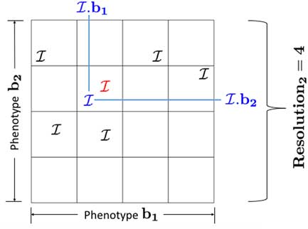
Figure 1 A simple representation of the MAP-Elites algorithm. At most one individual can be maintained in each bin. After simulation, the blue individual is placed in the same bin as the red individual, due to its phenotype, b. The individual with the higher fitness will be maintained. The other will be discarded
Algorithm 1 describes how MAP-Elites generates solutions; the process occurs in three stages: ‘creation’, ‘fill’, and ‘mutate’. The creation stage initializes all of the bins, each of which can hold a single individual (in this case, a set of weights to be given to the neural network for control) within a certain range of phenotypes.
The fill stage consists of generating random individuals, simulating those individuals, and placing them in the appropriate bin within the map. In the case of two individuals belonging to the phenotype range of the same bin, the more fit individual survives, while the other is discarded.
In contrast, during the mutate stage, one of the individuals within the map is randomly copied, mutated, and simulated. This mutation occurs by changing the individual’s genotype (weights of the neural network). Such a mutation will typically result in a change in phenotype evaluation, so the resulting individual may be placed in a different bin than the parent individual. In this way the map can continue to be filled during the mutate stage. This stage can continue until a stopping condition is met; in this work we choose a preset number of iterations and examine the final individuals after this process is complete.
The total number of individuals that can be maintained is equal to the number of bins, but in cases of lower phenotypic diversity in the population, fewer individuals may be maintained, as fewer bins are accessed. A major benefit of the MAP-Elites algorithm is that it not only preserves individuals with unique behaviors (because they may exist in a low-competition bin), but also that it encourages a spread of behaviors across the phenotype space. This may allow a system designer to better describe the shape of the fitness surface across phenotype dimensions.
2.3 Flight mechanics
In this section, we discuss the principles of aerodynamics utilized in the flight simulator (Anderson, Reference Anderson2010). The following theory is used in conjunction with computational data for a NACA 2412 airfoil, as calculated by the XFOIL airfoil analysis software (Drela, Reference Drela2013).
The aerodynamic forces of lift (F L ) and drag (F D ) on an airfoil are a function of the axial shear stresses (A) and normal pressure (N), as well as the angle between the airfoil chord and the velocity vector, known as the angle of attack (α). Figure 2 depicts the directions that F L and F D act on the airfoil, as well as the total aerodynamic force, F A ; F L is always directed normal to the direction of the free stream velocity, V ∞, and F D is always in the direction of the V ∞. In the figure, ϕ represents the pitch of the airfoil with respect to the horizontal, and θ is the angle between V ∞ and the horizontal. Equations (1) and (2) describe the method of obtaining F L and F D :
 $$F_{L} {\,\equals\,}N\,\rm cos\,\alpha {\,\minus\,}\it A\,\rm sin\,\alpha $$
 $$F_{D} {\,\equals\,}N\,\rm sin\,\alpha {\,\plus\,} \it A\,\rm cos\,\alpha $$
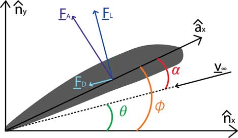
Figure 2 The aerodynamic force vectors which act the airfoil
These values describe the behavior of an airfoil under a specific set of conditions, and they are often used in their dimensionless forms, known as the coefficients of lift (C L ) and drag (C D ). They are calculated by dividing the forces by the planform area of the wing (s ref) and the free stream dynamic pressure (q ∞).
Calculations of s ref, q ∞, C L , and C D are as follows:
 $$s_{{{\rm ref}}} {\,\equals\,}c \cdot \ell $$
 $$q_{\infty} {\,\equals\,}{1 \over 2}\rho _{\infty} V_{\infty}^{2} $$
 $$C_{L} {\,\equals\,}{{F_{L} } \over {q_{\infty} s_{{{\rm ref}}} }}$$
 $$C_{D} {\,\equals\,}{{F_{D} } \over {q_{\infty} s_{{{\rm ref}}} }}$$
In the preceding equations, c is the average chord length of the wing and ρ ∞ the free stream air density. The force coefficients are thus dependent on the size and geometry of the wing, as well as the angle of attack, while remaining independent of the free stream air density and speed. With previously calculated values for C L and C D for varying α, F L and F D can be calculated using the following Equations (7) and (8):
 $$F_{L} {\,\equals\,}{1 \over 2} \cdot C_{L} \cdot V_{\infty}^{2} \cdot \rho _{\infty} \cdot s_{{{\rm ref}}} $$
 $$F_{D} {\,\equals\,}{1 \over 2} \cdot C_{D} \cdot V_{\infty}^{2} \cdot \rho _{\infty} \cdot s_{{{\rm ref}}} $$
It is an important note that V ∞ denotes the speed of the air in reference to the craft, which is often different from the speed of the craft with respect to the ground. This difference may be caused by the presence of wind, as is the case in our simulator.
Fixed-wing aircraft typically use propellers to create thrust, which acts parallel to the craft’s body, denoted as the
 $$\hat{a}_{x} $$
direction. In addition to controlling pitch, or rotation about the
$$\hat{a}_{x} $$
direction. In addition to controlling pitch, or rotation about the
 $$\hat{a}_{y} $$
, through use of the elevator, a craft can also control its rotation about the
$$\hat{a}_{y} $$
, through use of the elevator, a craft can also control its rotation about the
 $$\hat{a}_{x} $$
, known as roll, and rotation about the
$$\hat{a}_{x} $$
, known as roll, and rotation about the
 $$\hat{a}_{z} $$
, known as yaw. Figure 3 depicts the rigid frame used to describe the aircraft body. In this work, we use a simulator with 3 DOF: 2 linear (x and z) and 1 rotational (pitch about
$$\hat{a}_{z} $$
, known as yaw. Figure 3 depicts the rigid frame used to describe the aircraft body. In this work, we use a simulator with 3 DOF: 2 linear (x and z) and 1 rotational (pitch about
 $$\hat{a}_{y} $$
). For an aircraft to increase the amount of lift it can generate at a given speed, it can rotate about the
$$\hat{a}_{y} $$
). For an aircraft to increase the amount of lift it can generate at a given speed, it can rotate about the
 $$\hat{a}_{y} $$
axis to change α; Figure 4 displays the values of C
L
and C
D
used for a variety of α in the simulator (Drela, Reference Drela2013).
$$\hat{a}_{y} $$
axis to change α; Figure 4 displays the values of C
L
and C
D
used for a variety of α in the simulator (Drela, Reference Drela2013).
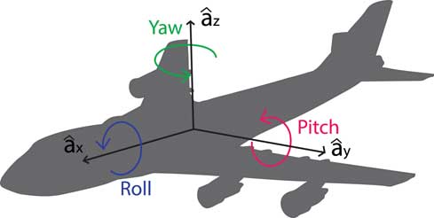
Figure 3 The rigid frame used to describe the aircraft
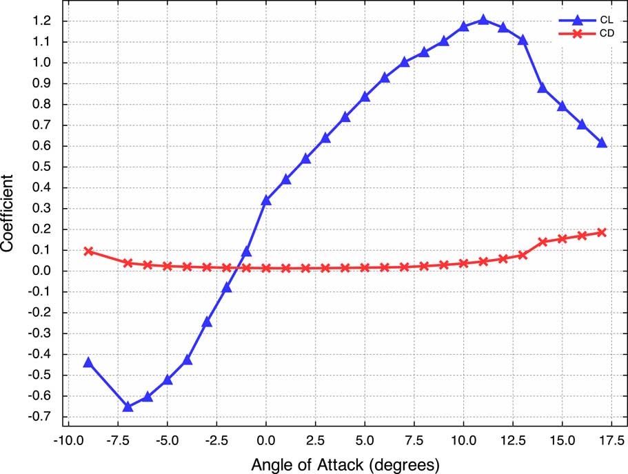
Figure 4 Plot of C L and C D for varying α on a NACA 2412 airfoil; GetCoefficients(α) returns these values
2.4 Related work
In this work, we study the use of the MAP-Elites search algorithm (Mouret & Clune, Reference Mouret and Clune2015) to develop successful weights for neural networks to act as control policies for a UAV in high-wind conditions. Autonomous flight and landing of UAVs has been a topic of interest for multiple decades (Foster & Neuman, Reference Foster and Neuman1970; Kim et al., Reference Kim, Jordan, Sastry and Ng2003; Green & Oh, Reference Green and Oh2006; Yliniemi et al., Reference Yliniemi, Agogino and Tumer2014b). As such, here we only provide a small sample of related works. For a more comprehensive view of autonomous UAV control, we refer the reader to Gautam et al.’s (Reference Gautam, Sujit and Saripalli2014) work; for MAP-Elites, the work by Mouret and Clune (Reference Mouret and Clune2015).
Most of the work on autonomous UAV control has consisted of model-based control schemes attempting to follow a pre-defined flight path. These control schemes can be either linear, linear with regime-switching, or nonlinear (Alexis et al., Reference Alexis, Nikolakopoulos and Tzes2011; Saeed et al., Reference Saeed, Younes, Islam, Dias, Seneviratne and Cai2015). In contrast, in this work we do not need a system model and instead use a search algorithm to develop weights for a neural network for model-free control.
Shepherd showed that an evolved neural network can outperform even a well-tuned linear controller with proportional, integral, and derivative gains (PID controller) for a quadrotor UAV; the craft was able to recover from disturbances of up to 180° (being turned upside-down), while a PID controller was only capable of recovering from disturbances of <60° (Shepherd & Tumer, Reference Shepherd and Tumer2010). In contrast, in this work we are performing a landing task with a fixed-wing UAV and using a different search mechanism.
Previous work on MAP-Elites has also been used to search for neural network weights for various tasks (Cully et al., Reference Cully, Clune, Tarapore and Mouret2015; Ecarlat et al., Reference Ecarlat, Cully, Maestre and Doncieux2015; Mouret & Clune, Reference Mouret and Clune2015). In this work we also search for neural network weights; however, the task in this work has unique dynamics compared to previous MAP-Elites studies and a strong sequential decision-making component.
3 Flight simulator design
To model UAV flight behavior, a 3 DOF flight simulator was designed for 2 linear and 1 rotational DOF. This 3 DOF simulator does not capture all dynamics (as a vehicle in flight has 6 DOF), but this more complex representation is beyond the scope of this work. The simulator approximates the effects of aerodynamic forces, while maintaining realistic aircraft behavior. It operates by receiving thrust and pitch controls, calculating the aerodynamic and gravitational forces on the aircraft, combining the forces, and calculating the system’s physical response. All pitching moments caused by aerodynamic forces are neglected due to the use of trim (Bauer, Reference Bauer1995) and C L and C D for varying α of the aircraft are based on that of a NACA 2412 airfoil, as predetermined using XFOIL (Drela, Reference Drela2013).
Algorithm 2, SimulateTimeStep, describes the main function of the simulator. While the time, t, is less than the maximum run time, t
max, the simulator provides the current state, S
t
, to the ANN through the function GetControls and receives the force and moment applied, F
C
and M
C
, respectively. The simulator then calculates V
∞ and θ from the aircraft’s ground speed in the 2 linear DOF,
 $$\dot{r}_{x} $$
and
$$\dot{r}_{x} $$
and
 $$\dot{r}_{z} $$
, and the wind generator. The average peak wind speed was ~15 m s−1, chosen to model the type of high winds that could shake a tree and would be difficult for a person to walk in (Lewis, Reference Lewis2011); a typical wind profile for a 30 seconds run can be seen in Figure 5. Using θ and S
t
, α, C
L
, and C
D
are calculated. After determining the aerodynamic forces on the aircraft, all of the forces are summed. The resultant force vector,
$$\dot{r}_{z} $$
, and the wind generator. The average peak wind speed was ~15 m s−1, chosen to model the type of high winds that could shake a tree and would be difficult for a person to walk in (Lewis, Reference Lewis2011); a typical wind profile for a 30 seconds run can be seen in Figure 5. Using θ and S
t
, α, C
L
, and C
D
are calculated. After determining the aerodynamic forces on the aircraft, all of the forces are summed. The resultant force vector, $\vec {F}_{R} $
, is put into the function DynamicsCalc along with S
t
and M
C
; thereby the new state,
$\vec {F}_{R} $
, is put into the function DynamicsCalc along with S
t
and M
C
; thereby the new state,
 $$S_{{t{\plus}t_{s} }} $$
, is determined.
$$S_{{t{\plus}t_{s} }} $$
, is determined.
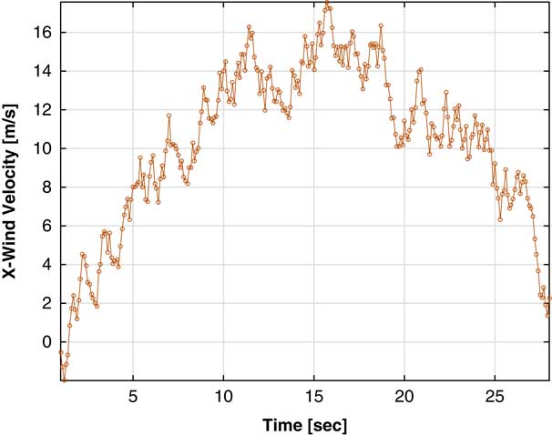
Figure 5 One sample of the simulator’s randomly generated wind; in this work we center the distribution around a sine function with amplitude 15 m s−1
The function DynamicsCalc, is described in detail in Algorithm 3. The algorithm was designed for scalability and therefore contains two loops: one for calculating linear system responses and another for calculating rotational system responses. The first loop runs through an iteration for each linear DOF, i; Newton’s first law of motion is used to calculate the acceleration,
 $$\ddot{r}_{{i,t{\plus}t_{s} }} $$
, then the aircraft’s velocity,
$$\ddot{r}_{{i,t{\plus}t_{s} }} $$
, then the aircraft’s velocity,
 $$\dot{r}_{{i,t{\plus}t_{s} }} $$
, and position,
$$\dot{r}_{{i,t{\plus}t_{s} }} $$
, and position,
 $$r_{{i,t{\plus}t_{s} }} $$
, are calculated using trapezoidal integration.
$$r_{{i,t{\plus}t_{s} }} $$
, are calculated using trapezoidal integration.
The second loop then performs an iteration for each rotational DOF, j. It calculates the aircraft’s angular acceleration,
 $$\ddot{\phi }_{{j,t{\plus}t_{s} }} $$
, and performs trapezoidal integration to calculate the aircraft’s angular velocity,
$$\ddot{\phi }_{{j,t{\plus}t_{s} }} $$
, and performs trapezoidal integration to calculate the aircraft’s angular velocity,
 $$\dot{\phi }_{{j,t{\plus}t_{s} }} $$
, and pitch,
$$\dot{\phi }_{{j,t{\plus}t_{s} }} $$
, and pitch,
 $$\phi _{{j,t{\plus}t_{s} }} $$
. Finally, all of the state variables form
$$\phi _{{j,t{\plus}t_{s} }} $$
. Finally, all of the state variables form
 $$S_{{t{\plus}t_{s} }} $$
, and the new state is returned.
$$S_{{t{\plus}t_{s} }} $$
, and the new state is returned.
4 Simulator verification
In order to verify that the flight simulator effectively models fixed-wing flight, we conducted preliminary experiments to test the functionality of the aerodynamic forces before introducing the neural network and MAP-Elites algorithm: a takeoff test and a stable flight test.
To ensure that the simulator properly calculates aerodynamic forces, we modeled a fixed-wing takeoff, and compared against the well-understood behavior of a fixed-wing craft. With ϕ=0, a constant thrust of 100 N was applied to the aircraft for 60 seconds. After approximately 14 seconds, at a speed of 70 m s−1, the aircraft lifted off, and continued to climb for the remainder of the simulation. The simulation was then repeated with ϕ increased to 5°, then 10° with respect to the horizontal. A plot of the horizontal and vertical displacements of the three simulations is shown in Figure 6. For the three simulations, as ϕ increases, the total horizontal displacement required for takeoff to occur decreases, which agrees with aerodynamic theory. To verify lift for both positive and negative α, ϕ was set to −10° with respect to the horizontal, and the same test was performed, this time allowing the thrust to act for a total of 8 minutes. Due to the negative coefficient of lift associated with this negative angle of attack, the aircraft never lifts off, thus validating the aerodynamic lift forces of the simulator for both positive and negative α.
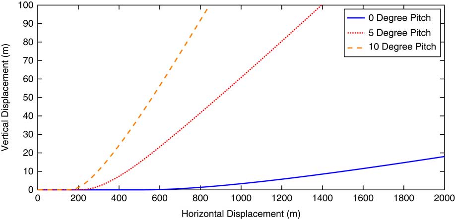
Figure 6 x- vs. z-position during the takeoff simulator verification test for 0, 5, and 10° constant ϕ
For the stable flight test, a force balance was first conducted on the aircraft to determine its horizontal equilibrium speed and equilibrium thrust at ϕ=0. Through algebraic manipulation, V ∞=69.3 m s−1 and F C =8.3 N were calculated for steady flight. These values were then used in the simulator for an aircraft already in the air, and the result was a bounded system that approached v z =0 with a maximum error of <0.01 mm s−1.
5 Experimental parameters
Our experimental runs used the following parameters: the UAV has a mass of 20 kg and a wing area of 0.2 m2, corresponding to a wingspan of 1 m and chord length of 20 cm. It has a rotational inertia of 20 kg m2. We initialize the UAV in low-level flight; it starts 25 m above the ground, with a 60 m s−1 x-velocity and 0 m s−1 z-velocity. To encourage landing in the early stages, we initialize the UAV pitched slightly downward, at ~3° below horizontal. The aircraft has full mobility through the space: it can climb without bound, and we observed some cases of the aircraft completing a full loop. The UAV is allowed up to 60 seconds of flight time, though the simulation is cut-off when the UAV touches down or when it reaches 200 m above ground level.
Our neural network used for control consisted of seven state inputs, five hidden units, and two control outputs. The state variables form the vector
 $$\{ t,\,\dot{r}_{x} ,\,\dot{r}_{z} ,\,r_{z} ,\,\dot{\phi },\,{\rm sin}\,(\phi ),{\rm cos}\,(\phi )\} $$
and are normalized using the ranges
$$\{ t,\,\dot{r}_{x} ,\,\dot{r}_{z} ,\,r_{z} ,\,\dot{\phi },\,{\rm sin}\,(\phi ),{\rm cos}\,(\phi )\} $$
and are normalized using the ranges
 $$\{ t\in{\minus}10\,\colon\,70,\,\dot{r}_{x} \in40\,\colon\,90,\,\dot{r}_{z} \in{\minus}10\,\colon\,10,\,r_{z} \in{\minus}5\,\colon\,30,\,\dot{\phi }\in{\minus}0.2\,\colon\,0.2,\,\rm sin\,(\phi )\in{\minus}0.5\,\colon\,0.5,} $$
 $$\,{\rm cos}\,(\phi )\in0\,\colon1\} $$
. We used five hidden units, because this allowed the search algorithm to discover successful policies while keeping the overall computation time low. The two control outputs are {F
C
, M
C
}, the force of thrust and the moment about the center of the wing. This force and moment is used for the dynamics of the time step. The UAV can provide thrust limited in the range 0:50 N, and a moment in the range 0:5 Nm.
$$\,{\rm cos}\,(\phi )\in0\,\colon1\} $$
. We used five hidden units, because this allowed the search algorithm to discover successful policies while keeping the overall computation time low. The two control outputs are {F
C
, M
C
}, the force of thrust and the moment about the center of the wing. This force and moment is used for the dynamics of the time step. The UAV can provide thrust limited in the range 0:50 N, and a moment in the range 0:5 Nm.
In our implementation of MAP-Elites, we represented each individual
 $$\left( {\cal I} \right)$$
as a set of weights for the neural network. We chose to use two phenotype dimensions with a resolution of 10 equally spaced bins along each dimension. This results in 100 empty bins at the start of each experimental trial. We used 50 filling iterations and 1000 mutation iterations.
$$\left( {\cal I} \right)$$
as a set of weights for the neural network. We chose to use two phenotype dimensions with a resolution of 10 equally spaced bins along each dimension. This results in 100 empty bins at the start of each experimental trial. We used 50 filling iterations and 1000 mutation iterations.
We examined a wide range of possible phenotypes, but found that the most effective phenotypes were those which averaged values across a moderate number of timesteps. For example, the final kinetic energy was a very sensitive phenotype; very small genotype (neural network weight) changes caused very large changes in the phenotype space. In contrast, using the average kinetic energy over the last 2–3 seconds (20–30 timesteps) proved to be more stable. In our results reported in this paper, we used the following two phenotypes:
-
∙ Phenotype 1: Average x-position over the last 2 seconds the UAV is in the air, with limits of 200:900 m.
-
∙ Phenotype 2: Average z-position over the last 2 seconds the UAV is in the air, with limits of 0:4 m.
We arrived at these phenotypic choices after a number of trials using other phenotypes including time-in-air, average x- or z-velocity over the last 2 seconds, final orientation, and average angle of attack over the last 2 seconds. We found that the final phenotypes we selected offer an interesting spread of behaviors for the following reasons: (1) preserving solutions which vary along the x-position before they land preserves solutions with longer-range approach behaviors which vary from conservative to aggressive, and (2) preserving solutions which vary in average z-positions before they land preserves solutions with close-to-ground behaviors which range from conservative to aggressive. We found that averaging over a short period of time before the UAV landed offered a more stable phenotype than simply choosing the final instantaneous velocity or position.
To calculate fitness of an individual, we use the angle at which the aircraft approaches the ground (‘glide angle’) and the factor i L . The glide angle is calculated using the x- and z-velocities over the last 3 seconds in flight; this allows for a more consistent fitness calculation than using the final instantaneous glide angle. The i L indicator returns a value of 0 if the UAV has landed and a very large negative number if it has not. The fitness calculation is shown below:
 $${\cal P}{\,\equals\,}\mathop{\sum}\limits_{t{\,\equals\,}({\rm end}{\minus}3)\,\colon\,{\rm end}} {\,\minus\,}\left| {{\rm a}\,{\rm tan}\left( {{{\dot{r}_{{z,t}} } \over {\dot{r}_{{x,t}} }}} \right)} \right|{\plus}i_{L} $$
During our experiments, we noticed that the number of bins being filled were significantly lower than was expected and remained so no matter how we adjusted the outer limits of the MAP. We found that this was due to a co-variation between our phenotype variables. In order to achieve a wider variety of phenotype behaviors, as well as to allow the UAV to drastically change its behavior when near the ground, we developed a NGCS scheme. In this scheme an individual is described not by one set of weights for the neural network, but two separate sets of weights. The UAV uses one set of weights for the approach, and when it is <5 m above ground level and has a negative velocity in the z-direction, the second set of weights are used. This allows for the UAV to more easily learn the nonlinear behaviors that are necessary for a smooth landing; human pilots use 3° as a rule of thumb for the glide angle before ‘flaring’ when they are close to the ground. This flaring action consists of increasing their angle of attack in order to create more lift for a softer landing (Watson et al., Reference Watson, Hardy and Warner1983).
We performed separate trials with and without wind effects. In the trials with wind, we created a random distribution around a sine function with amplitude 15 m s−1 (Figure 5).
6 Results
We conducted experiments by using MAP-Elites to search for controllers that provided a smooth landing in four cases: (1) no wind, no NGCS, (2) with wind, no NGCS, (3) no wind, with NGCS, and (4) with wind, with NGCS. Specifically, we show:
-
∙ A typical whole population of final controllers for each case (Section 6.1; Figures 7–10).
-
∙ Mean and standard deviation (μ, σ) of controller performance across 30 statistical runs (Section 6.2; Table 1).
-
∙ The effect of the choice of phenotype on final performance and recommendations for phenotypes in dynamic domains (Section 6.3; Figure 11).
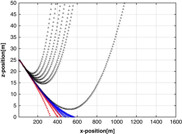
Figure 7 Case 1: Final flight profiles for a trial with no near-ground control switching, with no wind show the largest number of crafts that do not land
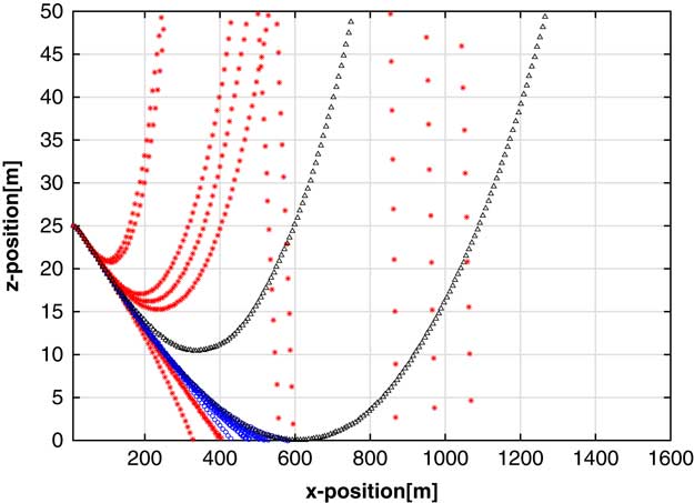
Figure 8 Case 2: Final flight profiles for a trial with no near-ground control switching, with wind
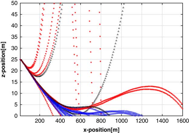
Figure 9 Case 3: Final flight profiles for a trial with near-ground control switching with no wind

Figure 10 Case 4: Final flight profiles for a trial with near-ground control switching with wind show the largest number of crafts with soft landings
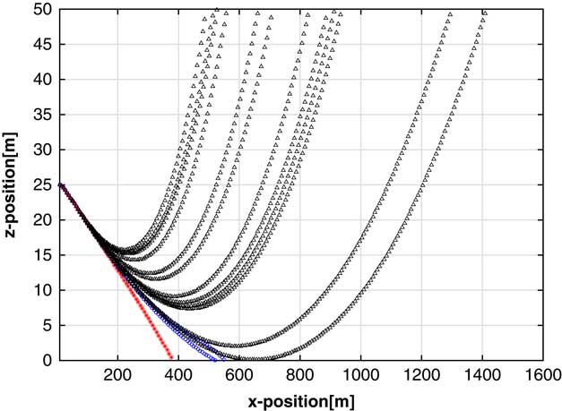
Figure 11 Final population flight profiles using the ϕ phenotypes
Table 1 Median number of solutions in the final map, mean, and standard deviation (μ, σ) of the landing glide angle, landing z-velocity, and landing x-velocity, for each wind/near-ground control switching (NGCS) combination and 100 randomly controlled trials
In each of the figures, a black path with triangles denotes that the UAV did not land within the allotted 60 seconds, a red path with asterisks denotes a hard landing with glide angle >3°, and a blue path with circles denotes a soft landing with glide angle <3°. The plots reflect the UAV’s x–z flight path.
6.1 Typical final population
The additional complexity of behaviors that can be learned by using the NGCS technique can best be seen by the flight profiles themselves. In Figures 7–10, we show the flight profiles of all members of the final population of a typical run for each method.
Figure 7 shows the final map population flights in the no NGCS, no wind case. The controllers that are developed can be easily described as ‘pull up, at various rates’. Seven of the generated controllers do not actually land over the 60 seconds of flight time, and instead climb until they reach the height bound, ending the simulation. Even though they are penalized heavily for not landing, they are protected as they have a sufficiently different phenotype from the others.
Figure 8 shows the final map population flights in the no NGCS, windy case. These controllers are also easily described as ‘pull up, at various rates’. In this case, the controllers are more proficient at making sure that their final z-location is at ground level, though this results in the undesirable behavior of ‘climb, stall, fall’. In an implementation, a system designer would use their knowledge to choose the best controller to implement, so the inclusion of these controllers in the final population is not a detriment. However, the stochastic nature of the wind showcases the primary weakness of this method: one controller gets as low as 0.05 m, but then continues to pull up and climbs without bound.
Figure 9 shows the final map population flights in the NGCS, no wind case. The phenotype protections still result in some controllers with the ‘climb, stall, fall’ profile; however, those that get close enough to the ground that NGCS takes effect have a much more sophisticated behavior than those without NGCS. These runs will level off, and sometimes briefly climb, but generally not without bound.
Figure 10 shows the final map population flights in the NGCS, windy case. These solutions are qualitatively similar to Figure 9, showing that the NGCS method in particular is good at rejecting the stochastic effects of the high winds.
6.2 Case profiles
We additionally performed 30 statistical trials for each wind, NGCS combination, as well as 100 flights with random control inputs. Table 1 shows the number of solutions generated and the mean and standard deviation {μ, σ} for the glide angle, landing z-velocity, and landing x-velocity. The values reported represent the values for controllers that landed with less than a 40° glide angle (to prevent ‘climb, stall, fall’ outliers from having a high impact on the σ calculations). In the random case, 60 of the 100 controllers landed, while 40 climbed without bound.
6.3 Recommendations for MAP-Elites in dynamic problems
Before concluding this work, we collate our experiences with MAP-Elites in a problem with a strong dynamics component, in order to provide guidelines for future researchers expanding the capabilities of MAP-Elites and related search algorithms in such problems. Our experiences have supported the following observations:
-
∙ Phenotype stability: When a small change in genotype leads to an extreme change in phenotype, we found that we did not achieve as high of a final performance. In a dynamic problem, averaging a few points around the time of interest—in this case the landing time—led to an increase in stability for the genotype–phenotype mapping. This leads to MAP-Elites performing more consistently across independent trials.
-
∙ Phenotype coupling: When phenotypes are coupled, the co-variation can prevent certain phenotype spaces in the map from being filled, or can preserve very low-fitness solutions for a long period of time.
-
∙ Phenotype limits: In this work, if a phenotype was outside our chosen limits for the map, it would be considered a part of the nearest bin. This had the benefit of not requiring any special handling for individuals with phenotypes outside of the limits, but also led to the preservation of some solutions that were well outside of the expected behaviors.
-
∙ Strong nonlinearities: If a desirable control scheme has strong nonlinearities or discontinuities, but the conditions in which these changes apply are easily described, defining an individual as a set of neural network weights can at least allow a greater spread in the phenotype space, if not increased average performance.
-
∙ Selection for mutation: Choosing the individual to mutate based on a uniform random over indexes will equally weight each individual; choosing based on a uniform random over phenotypes will weight those in rare portions of the phenotype space or those at the edges of clusters much more highly than those individuals that are surrounded in the phenotype space. We found a clear difference in selection probability, but not a clear difference in performance when testing both of these strategies. A fitness-biased selection (which we did not address in this work) will provide a more-greedy approach, which might not be beneficial (Lehman & Stanley, Reference Lehman and Stanley2011).
-
∙ Phenotype dimensions dictate behaviors: Figure 11 demonstrates that a moderately different choice in phenotypes can have a large impact on the system behavior. Here, we substituted the final angle, ϕ (averaged over 2 seconds, with range ±10°), for the x-position phenotype. The behavior is very qualitatively different. Despite using NGCS, only three of the produced solutions in this run actually land; all of the others climb without bound. This change in behaviors is a result of only a change in the phenotype used within MAP-Elites, demonstrating the importance of phenotype selection.
7 Conclusions
In this work we examined MAP-Elites for use as a search algorithm to generate successful controllers for autonomous UAVs, even with wind disturbances. We discovered that the most useful phenotypes were highly coupled, limiting the population that could be supported. We partially addressed this by introducing a second controller which is substituted when the UAV is <5 m above ground level and still traveling downward. This produced a wider variety of phenotypic behaviors and a median population twice as large. Our final controllers resulted in vertical landing speeds lower than dropping the aircraft from 50 cm above the ground. The softest landings had a glide angle of <1° and vertical speed of <1 m s−1.
These studies were limited by simulation-based factors: first, our simulation does not account for near-ground changes in aerodynamics and wind. Second, our simulation does not account for aerodynamic forces on the body, or any part of the aircraft when outside of the range which we could calculate coefficients of lift and drag using XFOIL. Finally, our simulation does not account for any changes in air pressure with altitude.
Future work on this topic includes implementing such a controller in a 6 DOF simulator, working toward physical implementation. We suspect that the solution quality we produced can be improved upon by casting the problem within the framework of multiple objectives and incorporating a framework that will allow optimization over those multiple objectives simultaneously (Yliniemi & Tumer, Reference Yliniemi and Tumer2014, Reference Yliniemi and Tumer2015). Additionally, we are researching MAP-Elites for more complex control problems, like vertical takeoff and landing of fixed-wing UAVs; small UAVs typically have a large enough thrust-to-weight ratio to be physically able to perform this maneuver, but it requires a skilled pilot to perform.
Acknowledgements
This material is based upon work supported by the National Aeronautics and Space Administration (NASA) Space Grant College and Fellowship Training Program Cooperative Agreement #NNX15AI02H, issued through the Nevada Space Grant. The authors would also like to thank the Nevada Advanced Autonomous Systems Innovation Center (NAASIC) for their continued support.


