2.1 Reinforcement learning

RL is a powerful machine learning paradigm, in which autonomous agents have the capability to learn through experience. An RL agent learns in an unknown environment, usually without any prior knowledge of how to behave. The agent receives a scalar reward signal r based on the outcomes of previously selected actions, which can be either negative or positive. Markov decision processes (MDPs) are considered the de facto standard when formalizing problems involving a single-agent learning sequential decision making (Wiering & van Otterlo, Reference Wiering and van Otterlo2012). A MDP consists of a reward function R, set of states S, set of actions A, and a transition function T (Puterman, Reference Puterman1994), that is a tuple 〈S, A, T, R〉. When in any state s∈S, selecting an action a∈A will result in the environment entering a new state s′∈S with probability T(s, a, s′)∈(0, 1), and give a reward r=R(s, a, s′).

An agent’s behaviour in its environment is determined by its policy π. A policy is a mapping from states to actions that determines which action is chosen by the agent for a given state. The goal of any MDP is to find the best policy (one which gives the highest expected sum of discounted rewards) (Wiering & van Otterlo, Reference Wiering and van Otterlo2012). The optimal policy for a MDP is denoted π*. Designing an appropriate reward function for the environment is important, as an RL agent will attempt to maximize the return from this function, which will determine the policy learned.

RL can be classified into two paradigms: model-based (e.g. Dyna, Rmax) and model-free (e.g. Q-Learning, SARSA). In the case of model-based approaches, agents attempt to learn the transition function T, which can then be used when making action selections. By contrast, in model-free approaches knowledge of T is not a requirement. Model-free learners instead sample the underlying MDP directly in order to gain knowledge about the unknown model, in the form of value function estimates (Q values). These estimates represent the expected reward for each state action pair, which aid the agent in deciding which action is most desirable to select when in a certain state. The agent must strike a balance between exploiting known good actions and exploring the consequences of new actions in order to maximize the reward received during its lifetime. Two algorithms that are commonly used to manage the exploration exploitation trade-off are ε-greedy and softmax (Wiering & van Otterlo, Reference Wiering and van Otterlo2012).

Q-Learning (Watkins, Reference Watkins1989) is one of the most commonly used RL algorithms. It a model-free learning algorithm that has been shown to converge to the optimum action-values with probability 1, so long as all actions in all states are sampled infinitely often and the action-values are represented discretely (Watkins & Dayan, Reference Watkins and Dayan1992). In Q-Learning, the Q values are updated according to the following equation:

(1) $$Q\left( {s,\,a} \right)\leftarrow Q\left( {s,\,a} \right){\plus}\alpha \Big[ {r{\plus}\gamma \,\mathop {{\rm max}}\limits_{a'} Q\left( {s',\,a'} \right)\,{\minus} \, Q\left( {s,\,a} \right)} \Big]$$

where a∈[0, 1] is the learning rate and γ∈[0, 1] is the discount factor.

2.2 Multi-agent reinforcement learning

The single-agent MDP framework becomes inadequate when we consider multiple autonomous learners acting in the same environment. Instead, the more general SG may be used in the case of a MAS (Buşoniu et al., Reference Buşoniu, Babuška and Schutter2010). A SG is defined as a tuple 〈S, A _{1 … N} , T, R _{1 … N} 〉, where N is the number of agents, S the set of states, A _i the set of actions for agent i (and A the joint action set), T the transition function, and R _i the reward function for agent i.

The SG looks very similar to the MDP framework, apart from the addition of multiple agents. In fact, for the case of N=1 a SG then becomes a MDP. The next environment state and the rewards received by each agent depend on the joint action of all of the agents in the SG. Note also that each agent may receive a different reward for a state transition, as each agent has its own separate reward function. In a SG, the agents may all have the same goal (collaborative SG), totally opposing goals (competitive SG), or there may be elements of collaboration and competition between agents (mixed SG).

One of two different approaches is typically used when RL is applied to MAS: multiple individual learners or joint action learners. In the former case multiple agents are deployed into a common environment, each using a single-agent RL algorithm, whereas joint action learners use multi-agent specific algorithms which take account of the presence of other agents. When multiple self-interested agents learn and act together in the same environment, it is generally not possible for all agents to receive the maximum possible reward. Therefore, MAS are typically designed to converge to a Nash equilibrium (Shoham et al., Reference Shoham, Powers and Grenager2007). While it is possible for multiple individual learners to converge to a point of equilibrium, there is no theoretical guarantee that the agents will converge to a Pareto optimal joint policy.

2.3 Reward shaping

RL agents typically learn how to act in their environment guided by the reward signal alone. Reward shaping provides a mechanism to guide an agent’s exploration of its environment, via the addition of a shaping signal to the reward signal naturally received from the environment. The goal of this approach is to increase learning speed and/or improve the final policy learned. Generally, the reward function is modified as follows:

(2) $$R'\,{\equals}\,R{\plus}F$$

where R is the original reward function, F the additional shaping reward, and R′ the modified reward signal given to the agent.

Empirical evidence has shown that reward shaping can be a powerful tool to improve the learning speed of RL agents; however, it can have unintended consequences. A classic example of reward shaping gone wrong is reported by Randløv and Alstrøm (Reference Randløv and Alstrøm1998). The authors designed an RL agent capable of learning to cycle a bicycle towards a goal, and used reward shaping to speed up the learning process. However, they encountered the issue of positive reward cycles due to a poorly designed shaping function. The agent discovered that it could accumulate a greater reward by cycling in circles continuously to collect the shaping reward encouraging it to stay balanced, than it could by reaching the goal state. As we discussed earlier, an RL agent will attempt to maximize its long-term reward, so the policy learned depends directly on the reward function. Thus, shaping rewards in an arbitrary fashion can modify the optimal policy and cause unintended behaviour.

Ng et al. (Reference Ng, Harada and Russell1999) proposed PBRS to deal with these shortcomings. When implementing PBRS, each possible system state has a certain potential, which allows the system designer to express a preference for an agent to reach certain system states. For example, states closer to the goal state of a problem domain could be assigned higher potentials than those that are further away. Ng et al. (Reference Ng, Harada and Russell1999) defined the additional shaping reward F for an agent receiving PBRS as shown in the following Equation:

(3) $$F\left( {s,\,s'} \right)\,{\equals}\,\gamma {\rm \Phi }\left( {s'} \right)\,{\minus}\,{\rm \Phi }\left( s \right)$$

where Φ(s) is the potential function which returns the potential for a state s, and γ the same discount factor used when updating value function estimates. PBRS has been proven not to alter the optimal policy of a single-agent acting in infinite-horizon and finite-horizon MDPs (Ng et al., Reference Ng, Harada and Russell1999), and thus does not suffer from the problems of arbitrary reward shaping approaches outlined above. In single-agent RL, even with a poorly designed potential function, the worst case is that an agent may learn more slowly than without shaping but the final policy is unaffected.

However, the form of PBRS proposed by Ng et al. (Reference Ng, Harada and Russell1999) can only express a designer’s preference for an agent to be in a certain state, and therefore cannot make use of domain knowledge that recommends actions. Wiewiora et al. (Reference Wiewiora, Cottrell and Elkan2003) proposed an extension to PBRS called potential-based advice, that includes actions as well as states in the potential function. The authors propose two methods of potential-based advice: look-ahead advice and look-back advice. The former method defines the additional reward received F as follows:

(4) $$F\left( {s,\,a,\,s',\,a'} \right)\,{\equals}\,\gamma {\rm \Phi }\left( {s',\,a'} \right)\,{\minus}\,{\rm \Phi }\left( {s,\,a} \right)$$

Wiewiora et al. (Reference Wiewiora, Cottrell and Elkan2003) provided a proof of policy invariance for look-ahead advice for single-agent learning scenarios. No corresponding proof has been provided for look-back advice, although empirical results suggest that this method also does not alter the optimal policy in single-agent learning scenarios. To maintain policy invariance when using look-ahead advice, the agent must choose the action that maximizes the sum of both Q value and potential:

(5) $$\pi \left( s \right)\,{\equals}\,argmax_{a} \left( {Q\left( {s,\,a} \right)\,{\plus}\,{\rm \Phi }\left( {s,\,a} \right)} \right)$$

where π(s) is the agent’s policy in state s (the action that will be chosen by the agent in state s). We will use Wieiwora’s look-ahead advice to test action-based heuristics in the experimental sections of this paper. From this point forth, we will use the abbreviations sPBRS and aPBRS to refer to PBRS approaches with state-based and action-based potential functions, respectively.

In MARL, work by Devlin and Kudenko (Reference Devlin and Kudenko2011) proved that PBRS does not alter the set of Nash equilibria of a SG. Furthermore, Devlin and Kudenko (Reference Devlin and Kudenko2012) also proved that the potential function can be changed dynamically during learning, while still preserving the guarantees of policy invariance and consistent Nash equilibria. PBRS does not alter the set of Nash equilibria of a MAS, but it can affect the joint policy learned. It has been empirically demonstrated that agents guided by a well-designed potential function can learn at an increased rate and converge to better joint policies, when compared to agents learning without PBRS (Devlin et al., Reference Devlin, Grzes and Kudenko2011a). However, with an unsuitable potential function, agents learning with PBRS can converge to worse joint policies than those learning without PBRS.

2.4 Multi-agent credit assignment structures

Here we introduce the MARL credit assignment structures that we will evaluate in the experimental sections of this paper. Two typical reward functions for MARL exist: local rewards unique to each agent and global rewards representative of the group’s performance. In addition to these basic credit assignment structures, we also evaluate the performance of several other shaped reward functions.

A local reward (L _i ) is based on the utility of the part of a system that agent i can observe directly. Individual agents are self-interested, and each will selfishly seek to maximize its own local reward signal, often at the expense of global system performance when locally beneficial actions are in conflict with the optimal joint policy.

A global reward (G) provides a signal to the agents which is based on the utility of the entire system. Rewards of this form encourage all agents to act in the system’s interest, with the caveat that an individual agent’s contribution to the system performance is not clearly defined. All agents receive the same reward signal, regardless of whether their actions actually improved the system performance.

A difference reward (D _i ) is a shaped reward signal that aims to quantify each agent’s individual contribution to the system performance (Wolpert et al., Reference Wolpert, Wheeler and Tumer2000). The unshaped reward is R=G(z), and the shaping term is F=−G(z _−i ). Formally:

(6) $$D_{i} \left( z \right)\,{\equals}\,G\left( z \right)\,{\minus}\,G\left( {z_{{\,{\minus}\,i}} } \right)$$

where D _i is the reward received by agent i, G(z) the global system utility, and G(z _−i ) referred to as the counterfactual. The counterfactual term represents the global utility for a theoretical system without the contribution of agent i. Here z is a general term that may represent either states or state action pairs, depending on the specific application. Difference rewards are a well-established shaping methodology, with many successful applications in MARL (e.g. Wolpert & Tumer, Reference Wolpert and Tumer2002; Tumer & Agogino, Reference Tumer and Agogino2007; Mannion et al., Reference Mannion, Mason, Devlin, Duggan and Howley2016d).

Counterfactual as potential (CaP), proposed by Devlin et al. (Reference Devlin, Yliniemi, Kudenko and Tumer2014), is an automated method of generating multi-agent potential functions using the same knowledge represented by difference rewards. CaP automatically assigns potentials to states using the counterfactual term G(z _−i ), so that Φ(s)=G(z _−i ). In this framework, the unshaped reward R=G(z), and the shaping reward F is calculated as normal in PBRS according to Equation (3). As Φ(s) for agent i is in fact based on the state of the other agents in the system, the potential function is dynamic, and CaP is thus an instance of dynamic PBRS (Devlin & Kudenko, Reference Devlin and Kudenko2012). CaP therefore preserves the guarantee of consistent Nash equilibria, while incorporating knowledge based on difference rewards in an automated manner.

3.1 Problem description

In this section we introduce the TCD, a SG designed with the intent of studying resource dilemmas using the MAS paradigm. As mentioned earlier, this domain was inspired by N-player dilemmas and resource dilemmas from the field of Game Theory. An example of a simple dilemma is the Prisoner’s Dilemma (Binmore, Reference Binmore2012), a well-studied problem in which two players (agents) have the options to either cooperate or defect. Mutual cooperation results in the highest global utility; however, if one player defects he receives a higher reward, while the cooperating player receives the sucker’s payoff. If both players choose to defect, they both receive a low payoff. The principles of the Prisoner’s Dilemma can be extended to N-player dilemmas, where N players must choose to cooperate or defect (Binmore, Reference Binmore2012).

Resource dilemmas are an example of an N-player dilemma, where multiple self-interested agents share a common resource, and each seeks to maximize its own returns. Agents may cooperate to conserve the resource and utilize it in a sustainable manner, or they may defect and selfishly attempt to extract the maximum value possible from the resource. When a majority of agents act conservatively, there is an incentive for agents to defect so that they will receive a better than average payoff.

However, as more agents choose to defect the resource becomes over-exploited, and the global payoff is less than if all agents cooperate. Furthermore, when over-exploitation becomes the norm there is no incentive for a self-interested agent to act conservatively; to do so would reduce the individual’s payoff. The dominant strategy is thus to defect but, paradoxically, if all agents cooperate they maximize the collective benefit, and each does better than if all play the dominant strategy.

There are numerous real world examples of resource or commons dilemmas; any natural resource that is owned and used in common by multiple entities presents a dilemma of how best to utilize it in a sustainable manner. Examples include fish stocks, wildlife, water resources, woodlands, and common pastures. There are also examples of negative commons, for example, atmospheric pollution or fraudulent activities, where an individual may benefit by damaging a common resource to the detriment of all.

Previous research into commons dilemmas has used approaches such as evolutionary computation (Howley & Duggan, Reference Howley and Duggan2011) and learning automata (de Jong & Tuyls, Reference de Jong and Tuyls2009) to develop cooperation among agents. In this empirical study, we explore the possibility of using PBRS to encourage cooperative strategies among self-interested RL agents. Agents learning using a local reward function L are purely self-interested, and seek to maximize their own utility. As a comparison and to provide an upper bound on possible performance, we have also tested agents using reward functions that are explicitly designed to maximize the system utility (the global reward function G and difference reward function D).

In the TCD, N agents each have the right to graze their livestock in a common pasture. At each timestep, the agents decide how many of their own animals will graze in the commons until the next timestep. Thus the action set for each agent is A={a _min, … , a _max}, where a _min and a _max correspond to the minimum and maximum number of animals that each agent is allowed to graze in the commons. The state for each agent is defined as the number of its own animals currently grazing in the commons. We define the occupancy of the commons ς as the sum of the animals placed in the commons by all agents n∈N at any particular time:

(7) $$\varsigma \,{\equals}\,\mathop{\sum}\limits_{n\,{\equals}\,1}^{n\,{\equals}\,N} {s_{n} } $$

Animals left grazing in the commons will increase in value between timesteps. We define χ as the increase in value for an animal left grazing in the commons for one timestep. However, there is a maximum number of animals the commons can sustain without deterioration from overgrazing. The capacity of the commons ψ is defined as the number of animals which can sustainably graze the commons without causing damage. Animals left grazing in the commons when it is at or below capacity will increase in value by the maximum χ _max. When the commons is over capacity, animals increase in value by a lower rate due to the lower quantity and quality of food available. The value of χ is related to the occupancy of the commons by the following equation:

(8) $$\chi \left( \varsigma \right)\,{\equals}\,\left\{ {\matrix{ {\chi _{{{\rm max}}} } \hfill & {if\,\varsigma \leq\psi } \hfill \cr {\chi _{{{\rm max}}} \,{\minus}\,{{\left( {\chi _{{{\rm max}}} \,{\minus}\,\chi _{{{\rm min}}} } \right){\times}\left( {\varsigma \,{\minus}\,\psi } \right)} \over {\varsigma _{{{\rm max}}} \,{\minus}\,\psi }}} \hfill & {otherwise} \hfill \cr } } \right.$$

Thus, the global benefit is maximized when ς=ψ, as all animals in the commons increase in value by the maximum rate. Values of ς that are less than ψ do not utilize the resource to its full potential, whereas values of ς greater than ψ result in damage to the resource, and a corresponding decrease in the collective benefit. Agents which select actions ⩽ $${\psi \over N}$$ are acting in a fair and conservative manner, analogously to the agents who choose to cooperate in the earlier example. Whereas agents who choose actions > $${\psi \over N}$$ are acting in an unfair and exploitative manner, similarly to agents who choose to defect in a classic N-player dilemma.

We use the commons value as a measure for the system utility, where the commons value for an episode is the sum of the products of χ and ς for each timestep. The relationship between the commons value and ς for the parameter values that we have chosen for our experiments is shown in Figure 1.

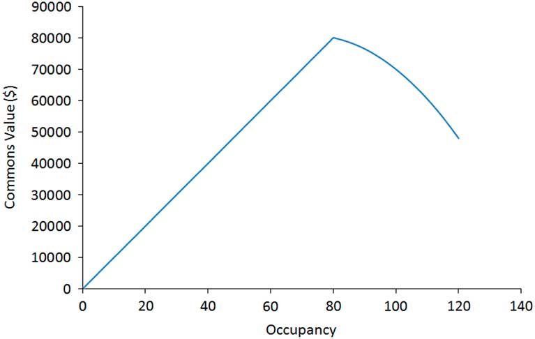
Figure 1 Occupancy vs. commons value for an entire episode of the tragic commons domain

The local reward for a self-interested agent i is calculated based on the added value per animal multiplied by the number of animals the agent currently has in the commons. Formally:

(9) $$L_{i} \left( {s_{i} ,a_{i} ,s'_{i} } \right)\,{\equals}\,\chi \left( {\varsigma '} \right)s'_{i} $$

The global reward is calculated based on the added value per animal multiplied by the total number of animals in the commons. This is a per-timestep version of the commons value metric that is used to measure overall episode performance. Formally:

(10) $$G\left( z \right)\,{\equals}\,\chi \left( {\varsigma '} \right)\varsigma '$$

The counterfactual for agent i, to be used with D and CaP, is calculated by assuming that the agent chose the same action as in the previous timestep, that is, a=s=s′. This means that a counterfactual occupancy ς(z _−i ) and a counterfactual animal value χ(z _−i ) must be calculated. The counterfactual term is then calculated as the product of ς(z _−i ) and χ(z _−i ). Formally:

(11) $$\varsigma \left( {z_{{\,{\minus}\,i}} } \right)\,{\equals}\,\mathop{\sum}\limits_{{\scriptstyle n\,{\equals}\,1 \atop \scriptstyle n\,\ne\,i} }^{n\,{\equals}\,N} {s'_{n} \,{\plus}\,s_{i} } $$

(12) $$\chi \left( {z_{{\,{\minus}\,i}} } \right)\,{\equals}\,\chi \left( {\varsigma \left( {z_{{\,{\minus}\,i}} } \right)} \right)$$

(13) $$G\left( {z_{{\,{\minus}\,i}} } \right)\,{\equals}\,\chi \left( {z_{{\,{\minus}\,i}} } \right)\varsigma \left( {z_{{\,{\minus}\,i}} } \right)$$

3.2 Potential-based reward shaping heuristics

To explore the effectiveness of PBRS in this domain, we apply three different manual heuristics in addition to the automated CaP heuristic. Each heuristic is expressed in both a state-based and action-based form. The heuristics used are:

• ∙ Fair: Agents are encouraged to act in a fair manner, where each agent is encouraged to graze the optimal number of animals (i.e. $${\psi \over N}$$ ) in the commons. This heuristic is expected to perform extremely well, and will demonstrate the effect of PBRS when advice can be given about the optimal policy.

  (14) $$\Phi \left( s \right)\,{\equals}\,\left\{ {\matrix{ {{{\psi \chi _{{{\rm max}}} } \over N}} \hfill & {if\,s\,{\equals}\,{\psi \over N}} \hfill \cr 0 \hfill & {otherwise} \hfill \cr } } \right.$$
  (15) $$\Phi \left( {s,\,a} \right)\,{\equals}\,\left\{ {\matrix{ {{{\psi \chi _{{{\rm max}}} } \over N}} \hfill & {if\,a\,{\equals}\,{\psi \over N}} \hfill \cr 0 \hfill & {otherwise} \hfill \cr } } \right.$$

• ∙ Opportunistic: Agents opportunistically seek to utilize any spare capacity available in the commons. As the available spare capacity is dependent on the joint actions of all agents in the system, the value of this potential function changes over time. Thus, this heuristic is an instance of dynamic PBRS (Devlin & Kudenko, Reference Devlin and Kudenko2012). This is a weaker shaping than Fair, and is included to demonstrate the effect of PBRS with a sub-optimal heuristic, for contexts where the optimal policy is not known.

  (16) $$\Phi \left( s \right)\,{\equals}\,\left\{ {\matrix{ {s\chi _{{{\rm max}}} } & {if\,\varsigma \,\lt\,\psi } \cr 0 \hfill & {otherwise} \cr } } \right.$$
  (17) $$\Phi \left( {s,\,a} \right)\,{\equals}\,\left\{ {\matrix{ {a\chi _{{{\rm max}}} } & {if\,\varsigma \,\lt\,\psi } \cr 0 \hfill & {otherwise} \cr } } \right.$$

• ∙ Greedy: Agents are encouraged to behave greedily, where each agent seeks to graze the maximum possible number of animals in the commons. This is an example of an extremely poor heuristic, and is expected to reduce the performance of all agents receiving it.

(18) $$\Phi \left( s \right)\,{\equals}\,\left\{ {\matrix{ {s_{{{\rm max}}} \chi _{{{\rm max}}} } \hfill & {if\,s\,{\equals}\,s_{{{\rm max}}} } \hfill \cr 0 \hfill & {otherwise} \hfill \cr } } \right.$$

(19) $$\Phi \left( {s,\,a} \right)\,{\equals}\,\left\{ {\matrix{ {a_{{{\rm max}}} \chi _{{{\rm max}}} } \hfill & {if\,a\,{\equals}\,a_{{{\rm max}}} } \hfill \cr 0 \hfill & {otherwise} \hfill \cr } } \right.$$

3.3 Experimental procedure

We test two variations of the TCD: a single-step version with num_timesteps=1 and a multi-step version with num_timesteps=12. The other experimental parameters used were as follows: num_episodes=20 000, N=20, ψ=80, χ _max=$1000/num_timesteps, χ _min=$400/num_timesteps, a _min=s _min=0, a _max=s _max=6, ς _max=120 (from Equation (7)). All agents begin each episode with their initial state set to 0 (i.e. no animals grazing in the commons).

We apply multiple individual Q-Learning agents to the TCD defined above, learning with credit assignment structures L, G, D, along with various shaping heuristics. The learning parameters for all agents are set as follows: α=0.20, γ=0.90, ε=0.10. Both α and ε are reduced by multiplication with their respective decay rates at the end of each episode, with alpha_decay_rate=0.9999 and epsilon_decay_rate=0.9999. These values were selected following parameter sweeps to determine the best performing settings. Each agent’s Q values for all state action pairs are initialized to 0 at the start of each experimental run.

Along with the MARL approaches tested, we have also conducted experiments with three simple agent types: Optimal, Random, and Greedy. Optimal agents always select the action equal to $${\psi \over N}$$ , and thus will maximize the global benefit. The random agents select actions randomly with equal probability. The greedy agents always select a _max, that is they play the dominant strategy, which is to graze as many animals as possible in the commons. Optimal and Greedy give the upper and lower performance bounds for this problem, and serve as a useful comparison to the MARL approaches tested.

3.4 Experimental results

For the single-step version of the problem, Figures 2(a)–2(d) show learning curves for commons value and occupancy for the approaches tested. For the multi-step version, Figures 3(a)–3(d) show learning curves for commons value and occupancy. The average performance of the approaches tested over the final 2000 episodes in both problem versions is shown in Table 1.

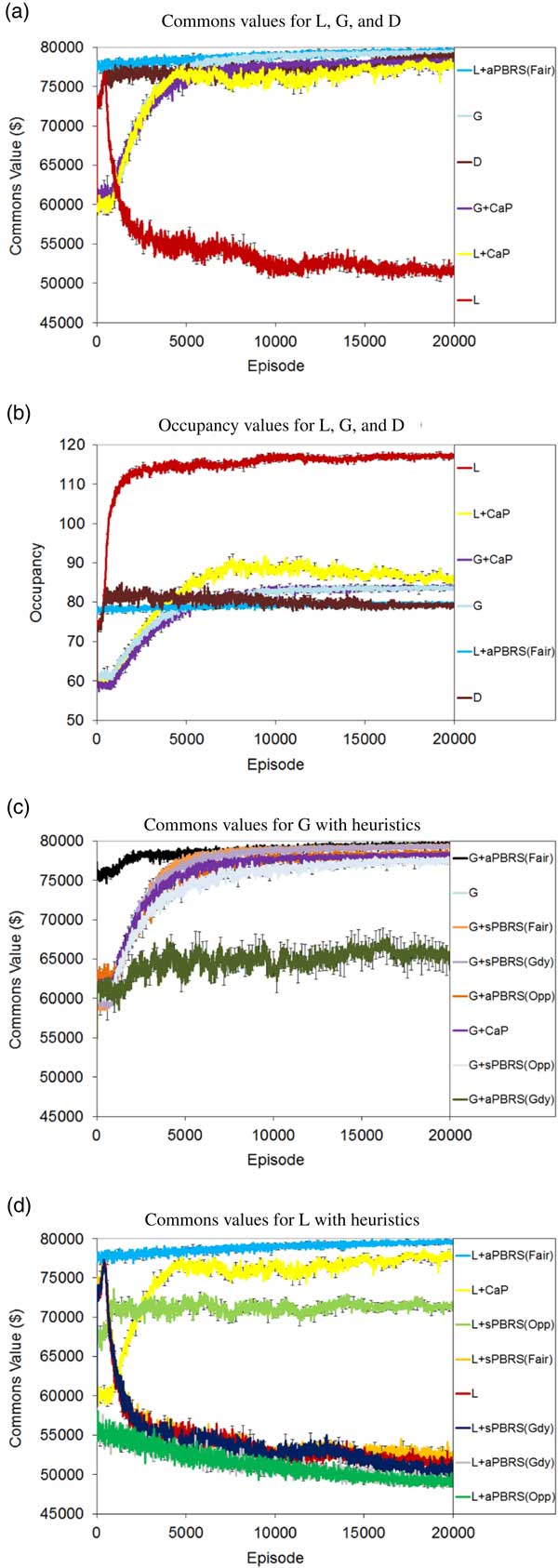
Figure 2 Single-step tragic commons domain results. (a) Commons values for L, G, and D. (b) Occupancy values for L, G, and D. (c) Commons values for G with heuristics. (d) Commons values for L with heuristics. sPBRS and aPBRS refer to potential-based reward shaping (PBRS) approaches with state-based and action-based potential functions, respectively; CaP=counterfactual as potential

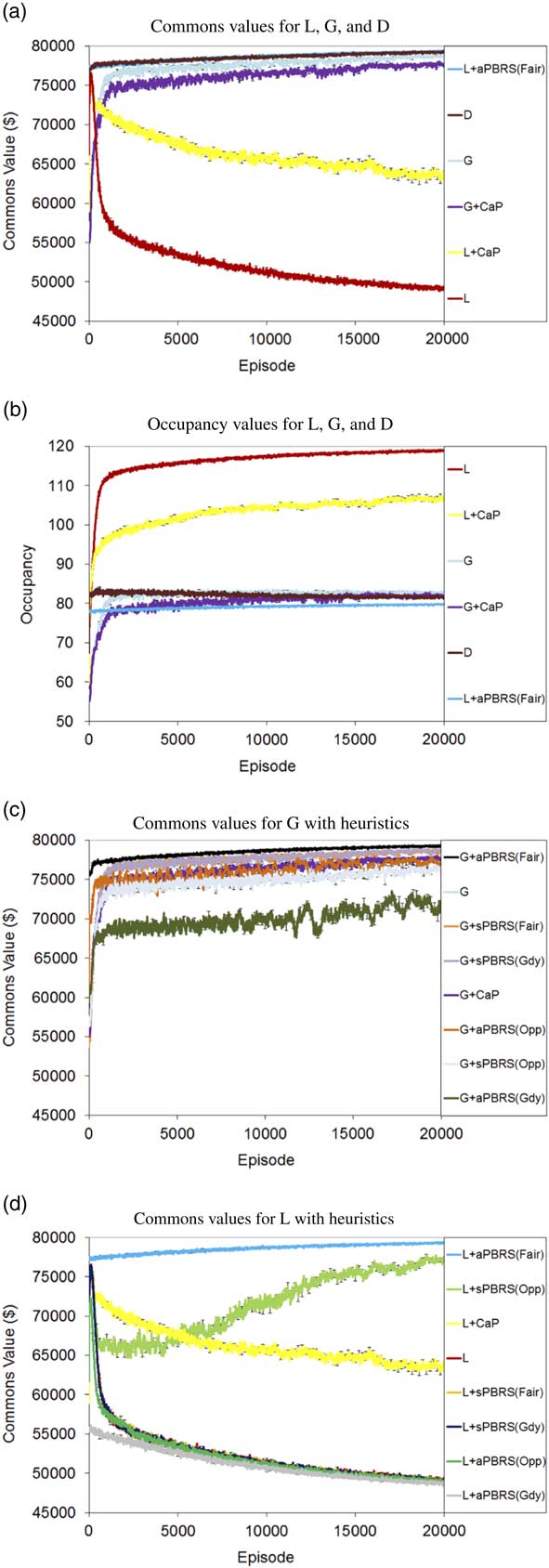
Figure 3 Multi-step tragic commons domain results. (a) Commons values for L, G, and D. (b) Occupancy values for L, G, and D. (c) Commons values for G with heuristics. (d) Commons values for L with heuristics. sPBRS and aPBRS refer to potential-based reward shaping (PBRS) approaches with state-based and action-based potential functions, respectively; CaP=counterfactual as potential

Table 1 Tragic commons domain results (averaged over last 2000 episodes)

sPBRS and aPBRS refer to potential-based reward shaping (PBRS) approaches with state-based and action-based potential functions, respectively; CaP=counterfactual as potential.

All plots include error bars representative of the standard error of the mean based on 50 statistical runs. Specifically, we calculate the error as $${\sigma \mathord{\left/ {\vphantom {\sigma {\sqrt n }}} \right. \kern-\nulldelimiterspace} {\sqrt n }}$$ , where σ is the standard deviation and n the number of statistical runs. Error bars are included on all plots at 200 episode intervals. The plots show the average performance across the 50 statistical runs that were conducted at 10 episode intervals. All claims of statistical significance are supported by two-tailed t-tests assuming unequal variances, with p=0.05 selected as the threshold for significance.

We can see from the learning curves that L starts out at quite a high level of performance, but this quickly degrades, eventually reaching a final policy close to that of the Greedy agents. The performance of L is significantly worse than the Random baseline in both the single-step (p=2.36×10⁻⁵⁷) and multi-step (p=2×10⁻¹⁰⁵) versions of the problem. Self-interested agents learning with L greedily seek to exploit the resource, as evidenced by the occupancy curves in Figures 2(b) and 3(b), where the agents consistently learn to graze close to the maximum allowed number of animals in the commons by the final training episodes.

By contrast, the approaches explicitly designed to maximize the global utility (G and D) perform quite well in the TCD. Rather than working at cross-purposes and seeking to exploit the resource to the maximum extent possible, agents learning using G and D converge to policies that utilize the shared resource in a fair and conservative manner, and both come close to the optimal level of performance in the single-step and multi-step variants of the problem. In both variants of the problem, D reaches a high level of performance very quickly, and learns more quickly than G. However, in the single-step TCD, G in fact reaches a higher final performance than D (99.2% of optimal performance for G vs. 98.5% of optimal performance for D). This difference in final performance was found to be statistically significant (p=0.025). D learned a better final policy than G in the multi-step version of the problem (99.0% of optimal performance for D vs. 98.3% of optimal performance for G). D was found to offer statistically better performance than G in the multi-step TCD (p=1.41×10⁻²³).

Devlin et al. (Reference Devlin, Yliniemi, Kudenko and Tumer2014) originally proposed CaP as a shaping heuristic for G; however, we have also tested L+CaP here in addition to the originally proposed G+CaP. G+CaP does not perform quite as well as G in either version of this problem domain. We find that CaP is a good heuristic for shaping L, reaching 97.1% of the optimal commons value in the single-step TCD, and 79.5% of the optimal commons value in the multi-step TCD. L+CaP offers a significant improvement over the Random baseline (and therefore unshaped L) in both the single-step (p=2.36×10⁻⁵⁷) and multi-step (p=1.47×10⁻¹¹) TCD.

The aPBRS(Fair) heuristic performs exceptionally well when combined with both L and G, in all cases reaching over 99% of the optimal commons value of $80 000. This is an extremely strong heuristic, that can guide even self-interested agents towards the optimal joint policy in the TCD. L+aPBRS(Fair) was found to offer statistically similar performance to G+aPBRS(Fair) in the single-step version (p=0.94), and statistically better performance than G+aPBRS(Fair) in the multi-step (p=2.7×10⁻⁶) version. The sPBRS(Fair) shaping performs well when combined with G, although not quite as well as G without shaping. L+sPBRS(Fair) performs quite similarly to L in both versions of the TCD. The aPBRS version of this heuristic is much more effective than the sPBRS version, as aPBRS specifies preferences for actions directly.

The sPBRS(Oppor.) heuristic is useful when combined with L to encourage behaviour leading to a high system utility. L+sPBRS(Oppor.) offers a significant improvement over the Random baseline (and therefore unshaped L) in both the single-step (p=3.69×10⁻³⁵) and multi-step (p=2.42×10⁻⁶⁶) TCD. G+sPBRS(Oppor.), however, does not reach the same performance as unshaped G in either variant of the TCD. The action-based version of this heuristic performs quite well when combined with G, although again not as well as the unshaped version of G. When combined with L, aPBRS(Oppor.) is among the worst performing approaches tested. This is because all agents are encouraged to graze the maximum number of animals in the commons when it is below capacity using this shaping, resulting in a lower overall return. By contrast, the sPBRS version performs better, as only agents that choose to add extra animals when the commons is below capacity are given the shaping reward.

The final PBRS heuristic that we tested was designed to encourage greedy behaviour in the agents, where each agent seeks to graze the maximum allowed number of animals in the commons. When combined with L, both the sPBRS and aPBRS versions of the greedy heuristic reach a lower final level of performance than unshaped L. The aPBRS version of this heuristic learns more quickly, again as the preferences for actions are defined directly. When combined with G, the sPBRS(Greedy) heuristic reduces the final performance by a small amount compared to unshaped G. G+aPBRS(Greedy) results in much lower performance than unshaped G in both versions of the TCD. As G is a much better performing reward function than L, the agents learning using G manage to overcome the incorrect knowledge that is provided to them, and to converge to reasonably good final policies. By contrast, the greedy heuristic serves to accentuate the self-interested nature of agents learning using L, especially in the case of L+aPBRS(Greedy).

4.1 Problem description

In this section we introduce a new multi-agent congestion game, the SPD. In the SPD, the agents must coordinate their actions to maximize the social welfare or global utility of the system. The SPD models a system of interconnected pastures, where each shepherd (agent) begins in a certain pasture and must decide in which pasture it will graze its herd of animals. At each timestep each agent knows which pasture it is currently attending and has the choice to remain still, or to move with its herd to an adjacent pasture.

Once all agents have completed their selected actions they are rewarded. Each pasture has a certain capacity ψ, and the highest reward for a pasture is received when the number of herds (agents) present is equal to the capacity of the pasture. Lower rewards are received for pastures which are congested as there is less food available to each herd, which affects the health and marketable value of the animals. Pastures that are under capacity also receive lower rewards, which reflects lost utility due to under-utilization of the resource. The local reward function (L) for a particular pasture is calculated as:

(20) $$L(s,\,t)\,{\equals}\,x_{t} e^{{{{\,{\minus}\,x_{{s,t}} } \over {\psi _{s} }}}} $$

where s is the pasture (state), x _s,t the number of herds (agents) present at that pasture at time t, and ψ _s the capacity of the pasture. The global reward or capacity utility can then be calculated as the summation of L(s, t) over all pastures in the SPD:

(21) $$G(t)\,{\equals}\,\mathop{\sum}\limits_{s \, \in \, S} {L\left( {s,\,t} \right)} $$

where S is the set of pastures in the SPD.

The difference reward (D) for an agent can be directly calculated by applying Equation (6). As an agent only influences the utility of the pasture it is currently attending at a particular timestep, D _i may be calculated as:

(22) $$D_{i} (t)\,{\equals}\,L(s,\,t)\,{\minus}\,(x_{{s,t}} \,{\minus}\,1)e^{{{{\,{\minus}\,(x_{{s,t}} \,{\minus}\,1)} \over {\psi _{s} }}}} $$

where x _s,t is the number of agents attending the same pasture s as agent i at timestep t. This evaluation is precisely equivalent to applying Equation (6) to Equation (21) directly. In a similar manner, the potential function for CaP may be calculated as:

(23) $$\Phi (s)\,{\equals}\,\left( {x_{{s,t}} \,{\minus}\,1} \right)e^{{{{\,{\minus}\,\left( {x_{{s,t}} \,{\minus}\,1} \right)} \over {\psi _{s} }}}} $$

Algorithm 1 provides additional details of the process followed in the SPD when agents are rewarded using G+CaP.

Other examples of congestion problems that have been studied thus far include the El-Farol bar problem (EBP) (Arthur, Reference Arthur1994), the traffic lane domain (TLD) (Tumer et al., Reference Tumer, Agogino and Welch2009) and the beach problem domain (BPD) (Devlin et al., Reference Devlin, Yliniemi, Kudenko and Tumer2014). All these approaches address the need to find solutions that maximize social welfare in systems with scarce resources. This is an important goal, due to the fact that insights gained while studying these problems may be useful when tackling congestion that occurs in real world systems, for example, in road, air, or sea transportation applications.

The SPD builds upon the work presented in these previous approaches, while introducing additional complexity. In the SPD, we consider two dimensional arrangements of resources, whereas resources are arranged in a single dimension only in the TLD and BPD. The arrangement of resources in the EBP is irrelevant to the outcome, as it is a stateless single shot problem where movement between resources is not allowed. The increased number of possible resource configurations leads to a larger number of available actions in the SPD (we consider up to five actions in our experiments), compared to three available actions in the BPD and TLD (move_left, stay_still, move_right). This increases the difficulty of the coordination task for the agents and thus the SPD allows for a more thorough evaluation of MARL approaches to tackling resource management problems. In this study, we consider a group of |S|=9 resources in a 3×3 grid arrangement. The 3×3 grid topology that we have used in our experiments is shown in Figure 4. Therefore, the actions available to the agents at each timestep are: stay_still, move_up, move_right, move_down, move_left. Actions which would move an agent outside the resource group leave its position unchanged. We set the number of agents N=100, and we assume that all resources have the same capacity ψ=4, and that N/4 agents start in each of the pastures 1, 3, 5, 7. The difficulty of this coordination problem could be increased further by assigning a random initial starting state to each agent at the beginning of each episode.

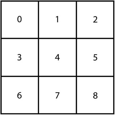
Figure 4 SPD 3×3 grid topology with resource (state) numbers

4.2 Potential-based reward shaping heuristics

To explore the effectiveness of PBRS in this domain, we apply four different manual heuristics in addition to the automated CaP heuristic. These four heuristics are based on those proposed by Devlin et al. (Reference Devlin, Yliniemi, Kudenko and Tumer2014) for the BPD, which we have adapted for the SPD. The work of Devlin et al. (Reference Devlin, Yliniemi, Kudenko and Tumer2014) is the only other study to date on the application of PBRS to congestion games, and we have included modified versions of these heuristics to test their effectiveness in congestion games with more complex resource configurations. Furthermore, Devlin et al. (Reference Devlin, Yliniemi, Kudenko and Tumer2014) expressed their heuristics in state-based forms only; therefore our work is the first empirical evaluation of aPBRS in congestion games. In the aPBRS heuristics below, the function next_state(s, a) returns the state that will be reached if an agent selects action a while in state s. The four heuristics that we have tested are:

• ∙ Overcrowd One: In the SPD, when the number of agents N is much greater than the combined capacity of the resources, the optimal solution is for N−(|S|−1)×ψ agents to converge to a single pasture, leaving ψ agents on each of the remaining pastures. This minimizes the effect of congestion on the system, and gives the highest possible social welfare (G=11.77). For the 3×3 grid instance of this domain with |S|=9 pastures of capacity ψ=4, this means that 68 agents must overcrowd one of the pastures so that the others remain uncongested. Overcrowd One promotes this behaviour, encouraging most of the agents to congest the middle pasture (s=4), and is therefore an extremely strong heuristic. It is important to note that this heuristic is manually tailored to individual agents. We expect this heuristic to achieve near-optimal performance, demonstrating the effectiveness of PBRS when precise information is available about the optimal joint policy.

  (24) $$\Phi (s)\,{\equals}\,\left( {\matrix{ {10} \hfill & {if\,s\,{\equals}\,0\,and\,agent\_id\in[0,\,\psi \,{\minus}\,1]} \hfill \cr {10} \hfill & {if\,s\,{\equals}\,1\,and\,agent\_id\in[\psi ,\,2\psi \,{\minus}\,1]} \hfill \cr {10} \hfill & {if\,s\,{\equals}\,2\,and\,agent\_id\in[2\psi ,\,3\psi \,{\minus}\,1]} \hfill \cr {10} \hfill & {if\,s\,{\equals}\,4\,and\,agent\_id\in[3\psi ,\,{N \mathord{\left/ {\vphantom {N 2}} \right. \kern-\nulldelimiterspace} 2}\,{\minus}\,\psi \,{\minus}\,1]} \hfill \cr {10} \hfill & {if\,s\,{\equals}\,3\,and\,agent\_id\in[{N \mathord{\left/ {\vphantom {N 2}} \right. \kern-\nulldelimiterspace} 2}\,{\minus}\,\psi ,\,{N \mathord{\left/ {\vphantom {N 2}} \right. \kern-\nulldelimiterspace} 2}\,{\minus}\,1]} \hfill \cr {10} \hfill & {if\,s\,{\equals}\,5\,and\,agent\_id\in[{N \mathord{\left/ {\vphantom {N 2}} \right. \kern-\nulldelimiterspace} 2},\,{N \mathord{\left/ {\vphantom {N 2}} \right. \kern-\nulldelimiterspace} 2}\,{\plus}\,\psi \,{\minus}\,1]} \hfill \cr {10} \hfill & {if\,s\,{\equals}\,4\,and\,agent\_id\in[{N \mathord{\left/ {\vphantom {N 2}} \right. \kern-\nulldelimiterspace} 2}\,{\plus}\,\psi ,\,N\,{\minus}\,3\psi \,{\minus}\,1]} \hfill \cr {10} \hfill & {if\,s\,{\equals}\,6\,and\,agent\_id\in[N\,{\minus}\,3\psi ,\,N\,{\minus}\,2\psi \,{\minus}\,1]} \hfill \cr {10} \hfill & {if\,s\,{\equals}\,7\,and\,agent\_id\in[N\,{\minus}\,2\psi ,\,N\,{\minus}\,\psi \,{\minus}\,1]} \hfill \cr {10} \hfill & {if\,s\,{\equals}\,8\,and\,agent\_id\in[N\,{\minus}\,\psi ,\,N\,{\minus}\,1]} \hfill \cr 0 \hfill & {otherwise} \hfill \cr } } \right.$$
  (25) $$\Phi (s,a)\,{\equals}\,\left( {\matrix{ {10} \hfill & {if\,next\_state(s,\,a)\,{\equals}\,0\,and\,agent\_id\in[0,\psi \,{\minus}\,1]} \hfill \cr {10} \hfill & {if\,next\_state(s,\,a)\,{\equals}\,1\,and\,agent\_id\in[\psi ,2\psi \,{\minus}\,1]} \hfill \cr {10} \hfill & {if\,next\_state(s,\,a)\,{\equals}\,2\,and\,agent\_id\in\left[ {2\psi ,\,3\psi \,{\minus}\,1} \right]} \hfill \cr {10} \hfill & {if\,next\_state(s,\,a)\,{\equals}\,4\,and\,agent\_id\in\left[ {3\psi ,\,{N \mathord{\left/ {\vphantom {N 2}} \right. \kern-\nulldelimiterspace} 2}\,{\minus}\,\psi \,{\minus}\,1} \right]} \hfill \cr {10} \hfill & {if\,next\_state(s,\,a)\,{\equals}\,3\,and\,agent\_id\in\left[ {{N \mathord{\left/ {\vphantom {N 2}} \right. \kern-\nulldelimiterspace} 2}\,{\minus}\,\psi ,\,{N \mathord{\left/ {\vphantom {N 2}} \right. \kern-\nulldelimiterspace} 2}\,{\minus}\,1} \right]} \hfill \cr {10} \hfill & {if\,next\_state(s,\,a)\,{\equals}\,5\,and\,agent\_id\in\left[ {{N \mathord{\left/ {\vphantom {N 2}} \right. \kern-\nulldelimiterspace} 2},\,{N \mathord{\left/ {\vphantom {N 2}} \right. \kern-\nulldelimiterspace} 2}\,{\plus}\,\psi \,{\minus}\,1} \right]} \hfill \cr {10} \hfill & {if\,next\_state(s,\,a)\,{\equals}\,4\,and\,agent\_id\in\left[ {{N \mathord{\left/ {\vphantom {N 2}} \right. \kern-\nulldelimiterspace} 2}\,{\plus}\,\psi ,\,N\,{\minus}\,3\psi \,{\minus}\,1} \right]} \hfill \cr {10} \hfill & {if\,next\_state(s,\,a)\,{\equals}\,6\,and\,agent\_id\in\left[ {N\,{\minus}\,3\psi ,\,N\,{\minus}\,2\psi \,{\minus}\,1} \right]} \hfill \cr {10} \hfill & {if\,next\_state(s,\,a)\,{\equals}\,7\,and\,agent\_id\in\left[ {N\,{\minus}\,2\psi ,\,N\,{\minus}\,\psi \,{\minus}\,1} \right]} \hfill \cr {10} \hfill & {if\,next\_state(s,a)\,{\equals}\,8\,and\,agent\_id\in\left[ {N\,{\minus}\,\psi ,\,N\,{\minus}\,1} \right]} \hfill \cr 0 \hfill & {otherwise} \hfill \cr } } \right.$$

• ∙ Middle: This heuristic incorporates some knowledge about the optimal policy, that is the idea that one resource should be ‘sacrificed’ or congested for the greater good of the system. However, in contrast to Overcrowd One this shaping is not tailored to individual agents, as all agents receive PBRS based on the same potential function. Thus, this heuristic encourages all agents to go to the middle pasture (s=4). We expect that this shaping will improve both the performance and learning speed of agents receiving PBRS, and will demonstrate the effect of PBRS when useful but incomplete domain knowledge is available.

  (26) $$\Phi (s)\,{\equals}\,\left\{ {\matrix{ {10} & {if\,s\,{\equals}\,4} \hfill\cr 0 \ & {otherwise} \cr } } \right.$$
  (27) $$\Phi (s,\,a)\,{\equals}\,\left\{ {\matrix{ {10} \hfill & {if\,next\_state(s,\,a)\,{\equals}\,4} \hfill \cr 0 \hfill & {otherwise} \hfill \cr } } \right.$$

• ∙ Spread: The Spread heuristic encourages agents to distribute themselves evenly across the pastures in the SPD. This is an example of a weak heuristic, and demonstrates the effect of PBRS in cases where very little useful domain knowledge is available. Therefore, we expect agents receiving this shaping to show modest if any improvements in learning speed and final performance.

  (28) $$\Phi (s)\,{\equals}\,\left( {\matrix{ {10} \hfill & {if\,s\,{\equals}\,0\,and\,agent\_id\in\left[ {0,\,{N \mathord{\left/ {\vphantom {N {\left| S \right|}}} \right. \kern-\nulldelimiterspace} {\left| S \right|}}\,{\minus}\,1} \right]} \hfill \cr {10} \hfill & {if\,s\,{\equals}\,1\,and\,agent\_id\in\left[ {{N \mathord{\left/ {\vphantom {N {\left| S \right|}}} \right. \kern-\nulldelimiterspace} {\left| S \right|}},\,{{2N} \mathord{\left/ {\vphantom {{2N} {\left| S \right|}}} \right. \kern-\nulldelimiterspace} {\left| S \right|}}\,{\minus}\,1} \right]} \hfill \cr {10} \hfill & {if\,s\,{\equals}\,2\,and\,agent\_id\in\left[ {{{2N} \mathord{\left/ {\vphantom {{2N} {\left| S \right|}}} \right. \kern-\nulldelimiterspace} {\left| S \right|}},\,{{3N} \mathord{\left/ {\vphantom {{3N} {\left| S \right|}}} \right. \kern-\nulldelimiterspace} {\left| S \right|}}\,{\minus}\,1} \right]} \hfill \cr {10} \hfill & {if\,s\,{\equals}\,3\,and\,agent\_id\in\left[ {{{3N} \mathord{\left/ {\vphantom {{3N} {\left| S \right|}}} \right. \kern-\nulldelimiterspace} {\left| S \right|}},\,{{4N} \mathord{\left/ {\vphantom {{4N} {\left| S \right|}}} \right. \kern-\nulldelimiterspace} {\left| S \right|}}\,{\minus}\,1} \right]} \hfill \cr {10} \hfill & {if\,s\,{\equals}\,4\,and\,agent\_id\in\left[ {{{4N} \mathord{\left/ {\vphantom {{4N} {\left| S \right|}}} \right. \kern-\nulldelimiterspace} {\left| S \right|}},\,{{5N} \mathord{\left/ {\vphantom {{5N} {\left| S \right|}}} \right. \kern-\nulldelimiterspace} {\left| S \right|}}\,{\minus}\,1} \right]} \hfill \cr {10} \hfill & {if\,s\,{\equals}\,5\,and\,agent\_id\in\left[ {{{5N} \mathord{\left/ {\vphantom {{5N} {\left| S \right|}}} \right. \kern-\nulldelimiterspace} {\left| S \right|}},\,{{6N} \mathord{\left/ {\vphantom {{6N} {\left| S \right|}}} \right. \kern-\nulldelimiterspace} {\left| S \right|}}\,{\minus}\,1} \right]} \hfill \cr {10} \hfill & {if\,s\,{\equals}\,6\,and\,agent\_id\in\left[ {{{6N} \mathord{\left/ {\vphantom {{6N} {\left| S \right|}}} \right. \kern-\nulldelimiterspace} {\left| S \right|}},\,{{7N} \mathord{\left/ {\vphantom {{7N} {\left| S \right|}}} \right. \kern-\nulldelimiterspace} {\left| S \right|}}\,{\minus}\,1} \right]} \hfill \cr {10} \hfill & {if\,s\,{\equals}\,7\,and\,agent\_id\in\left[ {{{7N} \mathord{\left/ {\vphantom {{7N} {\left| S \right|}}} \right. \kern-\nulldelimiterspace} {\left| S \right|}},\,{{8N} \mathord{\left/ {\vphantom {{8N} {\left| S \right|}}} \right. \kern-\nulldelimiterspace} {\left| S \right|}}\,{\minus}\,1} \right]} \hfill \cr {10} \hfill & {if\,s\,{\equals}\,8\,and\,agent\_id\in\left[ {{{8N} \mathord{\left/ {\vphantom {{8N} {\left| S \right|}}} \right. \kern-\nulldelimiterspace} {\left| S \right|}},\,N\,{\minus}\,1} \right]} \hfill \cr 0 \hfill & {otherwise} \hfill \cr } } \right.$$
  (29) $$\Phi (s,a)\,{\equals}\,\left( {\matrix{ {10} \hfill & {if\,next\_state(s,\,a)\,{\equals}\,0\,and\,agent\_id\in\left[ {0,\,{N \mathord{\left/ {\vphantom {N {\left| S \right|}}} \right. \kern-\nulldelimiterspace} {\left| S \right|}}\,{\minus}\,1} \right]} \hfill \cr {10} \hfill & {if\,next\_state(s,\,a)\,{\equals}\,1\,and\,agent\_id\in\left[ {{N \mathord{\left/ {\vphantom {N {\left| S \right|}}} \right. \kern-\nulldelimiterspace} {\left| S \right|}},\,{{2N} \mathord{\left/ {\vphantom {{2N} {\left| S \right|}}} \right. \kern-\nulldelimiterspace} {\left| S \right|}}\,{\minus}\,1} \right]} \hfill \cr {10} \hfill & {if\,next\_state(s,\,a)\,{\equals}\,2\,and\,agent\_id\in\left[ {{{2N} \mathord{\left/ {\vphantom {{2N} {\left| S \right|}}} \right. \kern-\nulldelimiterspace} {\left| S \right|}},\,{{3N} \mathord{\left/ {\vphantom {{3N} {\left| S \right|}}} \right. \kern-\nulldelimiterspace} {\left| S \right|}}\,{\minus}\,1} \right]} \hfill \cr {10} \hfill & {if\,next\_state(s,\,a)\,{\equals}\,3\,and\,agent\_id\in\left[ {{{3N} \mathord{\left/ {\vphantom {{3N} {\left| S \right|}}} \right. \kern-\nulldelimiterspace} {\left| S \right|}},\,{{4N} \mathord{\left/ {\vphantom {{4N} {\left| S \right|}}} \right. \kern-\nulldelimiterspace} {\left| S \right|}}\,{\minus}\,1} \right]} \hfill \cr {10} \hfill & {if\,next\_state(s,\,a)\,{\equals}\,4\,and\,agent\_id\in\left[ {{{4N} \mathord{\left/ {\vphantom {{4N} {\left| S \right|}}} \right. \kern-\nulldelimiterspace} {\left| S \right|}},\,{{5N} \mathord{\left/ {\vphantom {{5N} {\left| S \right|}}} \right. \kern-\nulldelimiterspace} {\left| S \right|}}\,{\minus}\,1} \right]} \hfill \cr {10} \hfill & {if\,next\_state(s,\,a)\,{\equals}\,5\,and\,agent\_id\in\left[ {{{5N} \mathord{\left/ {\vphantom {{5N} {\left| S \right|}}} \right. \kern-\nulldelimiterspace} {\left| S \right|}},\,{{6N} \mathord{\left/ {\vphantom {{6N} {\left| S \right|}}} \right. \kern-\nulldelimiterspace} {\left| S \right|}}\,{\minus}\,1} \right]} \hfill \cr {10} \hfill & {if\,next\_state(s,\,a)\,{\equals}\,6\,and\,agent\_id\in\left[ {{{6N} \mathord{\left/ {\vphantom {{6N} {\left| S \right|}}} \right. \kern-\nulldelimiterspace} {\left| S \right|}},\,{{7N} \mathord{\left/ {\vphantom {{7N} {\left| S \right|}}} \right. \kern-\nulldelimiterspace} {\left| S \right|}}\,{\minus}\,1} \right]} \hfill \cr {10} \hfill & {if\,next\_state(s,\,a)\,{\equals}\,7\,and\,agent\_id\in\left[ {{{7N} \mathord{\left/ {\vphantom {{7N} {\left| S \right|}}} \right. \kern-\nulldelimiterspace} {\left| S \right|}},\,{{8N} \mathord{\left/ {\vphantom {{8N} {\left| S \right|}}} \right. \kern-\nulldelimiterspace} {\left| S \right|}}\,{\minus}\,1} \right]} \hfill \cr {10} \hfill & {if\,next\_state(s,\,a)\,{\equals}\,8\,and\,agent\_id\in\left[ {{{8N} \mathord{\left/ {\vphantom {{8N} {\left| S \right|}}} \right. \kern-\nulldelimiterspace} {\left| S \right|}},\,N\,{\minus}\,1} \right]} \hfill \cr 0 \hfill & {otherwise} \hfill \cr } } \right.$$

• ∙ Overcrowd All: This heuristic encourages agents to go to slightly overcrowded pastures, and is an instance of dynamic PBRS (Devlin & Kudenko, Reference Devlin and Kudenko2012), as potentials of states or state action pairs may change over time. We expect this heuristic to perform poorly, and to serve as an example of the effect of PBRS when misleading information is used to design potential functions.

(30) $$\Phi (s)\,{\equals}\,\left\{ {\matrix{ {10} \hfill & {if\,\psi \,\lt\,x_{s} \,\lt\,2\psi } \hfill \cr 0 \hfill & {otherwise} \hfill \cr } } \right.$$

(31) $$\Phi (s,\,a)\,{\equals}\,\left\{ {\matrix{ {10} \hfill & {if\,\psi \,\lt\,x_{{next\_state(s,a)}} \,\lt\,2\psi } \hfill \cr 0 \hfill & {otherwise} \hfill \cr } } \right.$$

4.3 Experimental procedure

For all experiments, we plot the value of the global reward G (referred to as the capacity utility) against the number of completed learning episodes. All plots include error bars representative of the standard error of the mean based on 50 statistical runs. Specifically, we calculate the error as $${\sigma \mathord{\left/ {\vphantom {\sigma {\sqrt n }}} \right. \kern-\nulldelimiterspace} {\sqrt n }}$$ , where σ is the standard deviation and n the number of statistical runs. Error bars are included on all plots at 1000 episode intervals. The plots show the average performance across the 50 statistical runs that were conducted at 10 episode intervals. All claims of statistical significance are supported by two-tailed t-tests assuming unequal variances, with p=0.05 selected as the threshold for significance. In all experiments, the number of episodes is set to num_episodes=10 000, the number of timesteps is set to num_timesteps=1, the learning rate is set to α=0.1 with alpha_decay_rate=0.9999, the exploration rate is set to ε=0.05 with epsilon_decay_rate=0.9999 and the discount factor is set to γ=0.9. These parameter values were chosen to match those used by Devlin et al. (Reference Devlin, Yliniemi, Kudenko and Tumer2014) for the BPD.

4.4 Experimental results

Figures 5(a)–5(d) plot the learning curves for capacity utility for the approaches tested, while Table 2 gives the average capacity utility for each approach over the last 1000 episodes. In all plots the maximum possible capacity utility of 11.77 is marked with a black dashed line. In Table 2 we have also included several other results to serve as comparisons to the MARL approaches tested; these are: Optimum, Random Agents, Even Spread, Initial Distribution, and Worst. The Optimum figure shows the maximum possible capacity utility for the system, while Random Agents gives the average performance of 100 agents that select actions from a uniform random distribution in the SPD, averaged over 50 runs. Even Spread gives the capacity utility for the SPD if agents are evenly distributed among the pastures, and Initial Distribution gives the capacity utility for the starting conditions with N/4 agents in each of the pastures 1, 3, 5, 7. Finally, Worst gives the system utility if all 100 agents overcrowd any one of the nine pastures.

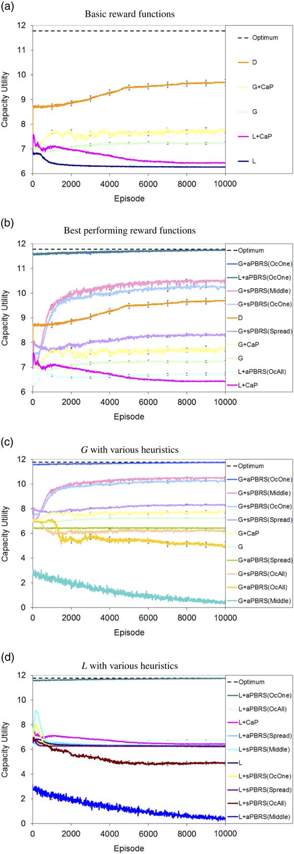
Figure 5 Shepherd problem domain results. (a) Basic reward functions. (b) Best performing reward functions. (c) G with various heuristics. (d) L with various heuristics. sPBRS and aPBRS refer to potential-based reward shaping (PBRS) approaches with state-based and action-based potential functions, respectively; CaP=counterfactual as potential

Table 2 Shepherd problem domain results (averaged over last 1000 episodes)

sPBRS and aPBRS refer to potential-based reward shaping (PBRS) approaches with state-based and action-based potential functions, respectively; CaP=counterfactual as potential.

The effectiveness of the approaches tested may be assessed by comparison with the performance of the Random Agents baseline. G significantly outperforms the Random Agents (p=4.43×10⁻¹¹), whereas L+aPBRS(OvercrowdAll) fails to outperform the Random Agents (p=1.1×10⁻⁵). Thus all approaches that perform better than G are also statistically better than choosing actions at random, whereas approaches that perform worse than L+aPBRS(OvercrowdAll) are in fact worse than selecting actions at random, and therefore demonstrate extremely poor performance in the SPD.

Figure 5(a) plots the performance of the typical MARL credit assignment structures L, G, and D, along with G+CaP and L+CaP. It is immediately apparent that all of these approaches fall far short of achieving the maximum possible performance in the SPD. D offers the best performance of these approaches, reaching a capacity utility of 9.68 or 82% of the maximum possible value. The CaP heuristic again proves to be useful in this problem domain, with G+CaP offering a statistically significant improvement in final performance compared to G (p=8.33×10⁻⁹), and L+CaP offering a statistically significant improvement in final performance compared to L (p=1.6×10⁻³⁷).

Figure 5(b) plots learning curves for the 10 reward functions with the best final performance. As we saw in the TCD study, aPBRS when combined with good heuristic information (Overcrowd One in this case) is again the best performer. This is of course to be expected, as Overcrowd One is an extremely strong heuristic that provides knowledge about the optimal policy for the SPD, and demonstrates again the effectiveness of aPBRS when good domain knowledge is available. G+sPBRS(Middle) is the next best performer, although its performance is statistically worse than G+aPBRS(OvercrowdOne) (p=2.96×10⁻²⁷). Nevertheless, G+sPBRS(Middle) still achieves a good level of performance, reaching a capacity utility of 10.50 or 89% of the optimal value. The Middle heuristic is, however, a more realistic evaluation of the effects of PBRS, as it is unlikely that precise information about the optimal policy (like that provided by Overcrowd One) will be available for every application domain. The performance of G+sPBRS(Middle) demonstrates that shaping with PBRS is effective even with less than perfect domain knowledge.

G+sPBRS(OvercrowdOne) performs statistically worse than G+sPBRS(Middle) (p=3.48×10⁻³); this is perhaps a surprising result, as the Overcrowd One heuristic provides more detailed information about how to behave on a per agent level. This can, however, be explained by the nature of shaping using sPBRS; agents receive shaping only upon reaching certain system states when implementing sPBRS. To exploit the knowledge provided by Overcrowd One fully, practically all agents would have to reach their encouraged position at the same time. It is interesting to note also that G+sPBRS(Middle) initially performs worse than G+sPBRS(OvercrowdOne); this is due to many of the agents initially being encouraged to converge on the middle state. G+sPBRS(Middle), however, quickly begins to outperform G+sPBRS(OvercrowdOne), as some agents select actions at random that lead to different states and thus higher system utilities, while the majority of agents converge on the middle state.

The performance of G+sPBRS(OvercrowdOne) is statistically better than D (p=4.57×10⁻⁵), and this demonstrates that for certain applications PBRS combined with good heuristic information is a suitable alternative to the now ubiquitous difference reward. Implementing PBRS with a manually specified heuristic for MARL also does not require precise knowledge of the mathematical form of the system evaluation function, whereas this is a requirement for D which could potentially be problematic for more complex application areas. Of course this shortcoming also affects the automated CaP PBRS heuristic, however, recent work on estimating counterfactuals (Colby et al., Reference Colby, Duchow-Pressley, Chung and Tumer2016) shows promise in addressing this limitation.