


1. Introduction
Agents acting in real worlds have to deal with uncertainty; therefore, any plan can become invalid at some point. An approach to address such a problem is to either anticipate all possible contingencies at planning time (e.g., through conformant or contingent planning models Smith & Weld, Reference Smith and Weld1998; Bonet, Reference Bonet2010) or deal with them as soon as something disruptive actually arises. When, however, there is no model about the uncertainty or the number of unexpected situations is not bounded, it is nevertheless necessary to have some mechanism to come up with a new course of actions. A solution to such a problem is replanning. That is, as soon as the agent recognizes that its plan does not work anymore, it formulates a new problem and computes new plans from that point onward.
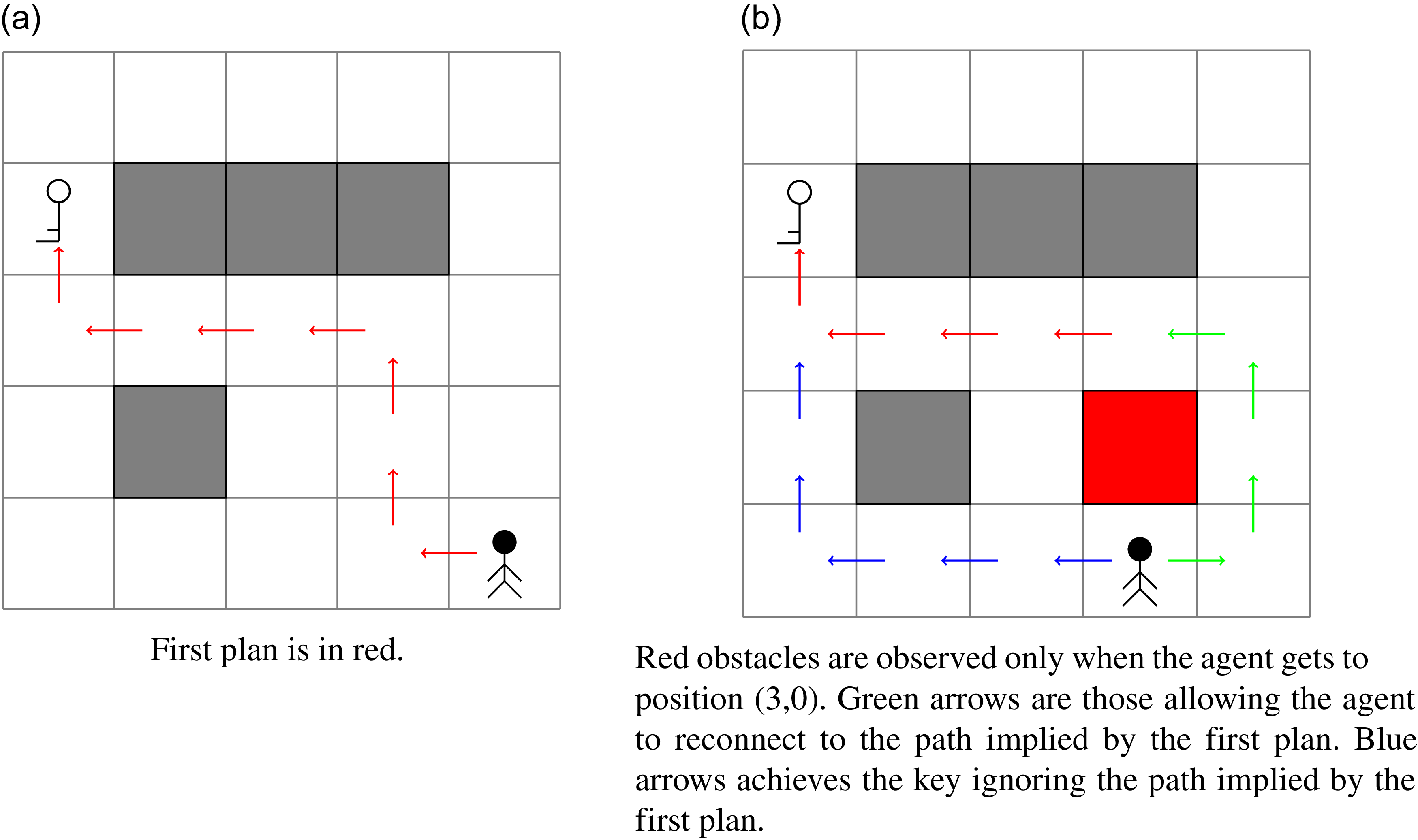
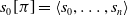
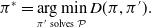
Although replanning can be effective in certain scenarios (Yoon et al., Reference Yoon, Fern and Givan2007; Ruml et al., Reference Ruml, Do, Zhou and Fromherz2011) and plan reuse can be even more challenging (Nebel & Koehler, Reference Nebel and Koehler1995), it is widely recognized that repairing the current course of action is often significantly more effective in practice (Gerevini & Serina, Reference Gerevini and Serina2010; Scala & Torasso, Reference Scala and Torasso2014). Not only can the plan be more easily recoverable so limiting the computational burden, but, also, the number of modifications to apply can be limited, therefore optimizing the stability of the system. Plan stability is important when humans have already validated the planning activities under execution, and the effort required for such a validation is considerable. In this case, stable plans reduce the cognitive load on human observers by ensuring coherence and consistency of behaviors (Fox et al., Reference Fox, Gerevini, Long and Serina2006). Consider for instance the example of Figure 1. We have an agent who needs to get a key somewhere in an environment. Unfortunately, while executing the plan shown in Figure 1(a), the agent is found to be in front of a wall that was not visible at planning time, as depicted in Figure 1(b). How we recover from that situation? Of course, the agent can compute a new plan (the blue arrows in Figure 1b), but such a plan has no guarantee to account for what the agent decided before. A more stable plan is instead the one starting with the green arrows (the part of the plan which was not computed before) followed by the red one (the part of the plan which was computed offline).
An agent moves in the cardinal directions trying to get to the key. (0,0) is the left most cell on the bottom, so the agent starts at position (4,0) and is tasked to go to position (0,3).
Previous solutions to the problem of repairing a plan have however no guarantees that the recovered plan is the most stable plan that can be computed (Koenig & Likhachev, Reference Koenig and Likhachev2002; van der Krogt & de Weerdt, Reference van der Krogt and de Weerdt2005; Fox et al., Reference Fox, Gerevini, Long and Serina2006; Gerevini & Serina, Reference Gerevini and Serina2010; Garrido et al., Reference Garrido2010; Scala, Reference Scala2014; Scala & Torasso, Reference Scala and Torasso2015; Höller et al., Reference Höller, Bercher, Behnke and Biundo2018; Goldman et al., Reference Goldman, Kuter and Freedman2020). Following on this line of research, in this paper, we take plan stability as the primary objective of the plan repair problem. In particular, we present a compilation-based approach that, given a planning problem and a plan, solves the plan repair problem with the guarantee of finding plans that are at the minimum distance from the input plan. We do so by making heavy use of a cost function that captures the implications of using actions that do not belong to the input plan, using extra occurrences of actions in the input plans, and that captures whenever the agent is not using actions in the input plan. More specifically, we focus our attention on using the plan distance metric defined by Fox et al. (Reference Fox, Gerevini, Long and Serina2006) as cost function. This distance is useful in all scenarios where the presence/absence of an action is a good proxy to understand the behavior of an agent; other scenarios can benefit from more powerful notions of distance, but we leave the study on how to deal with them computationally as a future investigation. The compilation we propose produces a classical planning problem that can be handled by any cost-sensitive planner.
In many applications, there may be multiple plans already validated by human experts, and all the accumulated experience stored in these plans is considered equally valuable and worth reusing. This is analogous to case-based planning, where a plan library can store multiple plans that solve the same problem (Muñoz-Avila & Cox, Reference Muñoz-Avila and Cox2008; Gerevini et al., Reference Gerevini, Roubcková, Saetti, Serina, Delany and Ontañón2013). So, in this paper we also tackle a new variant of the repair problem with the aim of finding a plan with minimum distance from a set of input plans. Like for the stability problem from a single plan, we addressed this problem by a compilation-based approach that computes the minimum distance plan w.r.t. any plan in the set of input plans.
To understand the practicability of our compilation, we report on an extensive experimental analysis comparing various optimal and satisficing planners with and without our compilation, over the planning problems from the 2018 edition of the planning competition, as well as with
 ${\mathsf{LPG}\textrm{-}\mathsf{adapt}}$
, a state-of-the-art system that natively repairs plans. Our results show that optimal plan repair is not only feasible but also competitive with greedy approaches, such as
${\mathsf{LPG}\textrm{-}\mathsf{adapt}}$
, a state-of-the-art system that natively repairs plans. Our results show that optimal plan repair is not only feasible but also competitive with greedy approaches, such as
 ${\mathsf{LPG}\textrm{-}\mathsf{adapt}}$
. Furthermore, it serves as an effective alternative to replanning from scratch across a wide range of domains.
${\mathsf{LPG}\textrm{-}\mathsf{adapt}}$
. Furthermore, it serves as an effective alternative to replanning from scratch across a wide range of domains.
This paper extends our initial work on the topic, that is, Saetti and Scala (Reference Saetti and Scala2022). In particular, we provide: (i) a complete running example that helps understanding the problem and the compilation solution that we study starting from the background, (ii) two variants of the compilation scheme that we initially proposed, one of which is a simplification of our initial scheme, while the other one works at a lifted level, (iii) an extension of the problem and compilation to the multi-plan case, that is, when we want to find the optimal stable plan trying to repair from a set of input plans, (iv) extended proofs showing the soundness, completeness, and optimality of our initial compilation scheme, as well as new proofs for the proposed variants of our initial scheme, (v) novel experiments, and (vi) a deeper related work analysis.
The paper starts with some background in Section 2 and provides the necessary definitions for the optimal repair problem in Section 3. Then, Sections 4 and 5 provide the compilation methods for the single and multi-plan repair case, together with soundness and completeness proofs. We end our paper with experiments (Section 7) and related work (Section 8).
2. Background
A planning domain
 ${\mathcal{D}}$
is a pair
${\mathcal{D}}$
is a pair
 $\langle P,O \rangle$
, where P is a set of predicates with associated arity of a first-order language, and O is a finite set of operators with associated arity. Predicates and operators of arity n are called n-ary predicates and n-ary operators. In the rest of the paper, we used both terms ‘lifted action’ and ‘operator’ interchangeably.
$\langle P,O \rangle$
, where P is a set of predicates with associated arity of a first-order language, and O is a finite set of operators with associated arity. Predicates and operators of arity n are called n-ary predicates and n-ary operators. In the rest of the paper, we used both terms ‘lifted action’ and ‘operator’ interchangeably.
We define an n-ary operator op as a tuple
 $\langle\mathsf{par}(op),\mathsf{pre}(op),\mathsf{eff}(op)\rangle$
, where
$\langle\mathsf{par}(op),\mathsf{pre}(op),\mathsf{eff}(op)\rangle$
, where
 $\mathsf{par}(op)$
is a tuple of n distinct variables
$\mathsf{par}(op)$
is a tuple of n distinct variables
 $\boldsymbol{x}=(x_1,\dots,x_n)$
,
$\boldsymbol{x}=(x_1,\dots,x_n)$
,
 $\mathsf{pre}(op)$
is a formula over P, and
$\mathsf{pre}(op)$
is a formula over P, and
 $\mathsf{eff}(op)$
is a consistent set of positive and negative literals over P.
$\mathsf{eff}(op)$
is a consistent set of positive and negative literals over P.
 $\mathsf{par}(op)$
,
$\mathsf{par}(op)$
,
 $\mathsf{pre}(op)$
, and
$\mathsf{pre}(op)$
, and
 $\mathsf{eff}(op)$
are called the parameters, preconditions, and effects of the operator op, respectively.
$\mathsf{eff}(op)$
are called the parameters, preconditions, and effects of the operator op, respectively.
The ground predicate
 $p(c_1,\dots,c_n)$
of a predicate
$p(c_1,\dots,c_n)$
of a predicate
 $p \in P$
that applies to n variables
$p \in P$
that applies to n variables
 $\boldsymbol{x}=(x_1,\dots,x_n)$
is obtained by replacing
$\boldsymbol{x}=(x_1,\dots,x_n)$
is obtained by replacing
 $x_i$
with constant
$x_i$
with constant
 $c_i$
for
$c_i$
for
 $i \in \{1, \dots, n\}$
. Similarly, the ground action
$i \in \{1, \dots, n\}$
. Similarly, the ground action
 $a=op(c_1,\dots,c_n)$
of an n-ary operator op w.r.t. constants
$a=op(c_1,\dots,c_n)$
of an n-ary operator op w.r.t. constants
 $c_1,\dots,c_n$
is the pair
$c_1,\dots,c_n$
is the pair
 $\langle \mathsf{pre}(a),\mathsf{eff}(a)\rangle$
, where
$\langle \mathsf{pre}(a),\mathsf{eff}(a)\rangle$
, where
 $\mathsf{pre}(a)$
(resp.
$\mathsf{pre}(a)$
(resp.
 $\mathsf{eff}(a)$
) is obtained by replacing the i-th parameter of
$\mathsf{eff}(a)$
) is obtained by replacing the i-th parameter of
 $\mathsf{par}(op)$
in
$\mathsf{par}(op)$
in
 $\mathsf{pre}(op)$
(resp.
$\mathsf{pre}(op)$
(resp.
 $\mathsf{eff}(op)$
) with
$\mathsf{eff}(op)$
) with
 $c_i$
for
$c_i$
for
 $i \in \{1, \dots, n\}$
. In the following, with
$i \in \{1, \dots, n\}$
. In the following, with
 $ \mathsf{eff}^+(a)$
and
$ \mathsf{eff}^+(a)$
and
 $ \mathsf{eff}^-(a)$
we indicate the positive and the negative effects of a. Moreover, we use the term object to refer to the constants used for grounding, refer to a ground predicate as a fact, and, for brevity, refer to a ground action simply as an action.
$ \mathsf{eff}^-(a)$
we indicate the positive and the negative effects of a. Moreover, we use the term object to refer to the constants used for grounding, refer to a ground predicate as a fact, and, for brevity, refer to a ground action simply as an action.
Let F be a set of facts, a state s is a subset of F with the meaning that if
 $ f \in s $
then f is true in s, otherwise it is false. An action a is applicable in s if and only if
$ f \in s $
then f is true in s, otherwise it is false. An action a is applicable in s if and only if
 $ s \models \mathsf{pre}(a) $
. The execution of an action a in s, denoted by s[a], generates a new state s ′ such that
$ s \models \mathsf{pre}(a) $
. The execution of an action a in s, denoted by s[a], generates a new state s ′ such that
 $ s' = (s \setminus \mathsf{eff}^-(a)) \cup \mathsf{eff}^+(a) $
.
$ s' = (s \setminus \mathsf{eff}^-(a)) \cup \mathsf{eff}^+(a) $
.
A classical planning problem
 $ {{{\mathcal{P}}}} $
of a planning domain
$ {{{\mathcal{P}}}} $
of a planning domain
 ${{{\mathcal{D}}}}$
and a set of constants
${{{\mathcal{D}}}}$
and a set of constants
 ${{{\mathcal{C}}}}$
is the tuple
${{{\mathcal{C}}}}$
is the tuple
 $ \langle F,A,I,G,c\rangle $
, where F is the set of facts obtained from
$ \langle F,A,I,G,c\rangle $
, where F is the set of facts obtained from
 ${{{\mathcal{C}}}}$
and the set of predicates P of
${{{\mathcal{C}}}}$
and the set of predicates P of
 ${{{\mathcal{D}}}}$
, A is a set of actions obtained from
${{{\mathcal{D}}}}$
, A is a set of actions obtained from
 ${{{\mathcal{C}}}}$
and the set of operators O of
${{{\mathcal{C}}}}$
and the set of operators O of
 ${{{\mathcal{D}}}}$
,
${{{\mathcal{D}}}}$
,
 $ I \subseteq F $
is a state called the initial state, G is a formula over F,
$ I \subseteq F $
is a state called the initial state, G is a formula over F,
 $ c\;:\; A \mapsto \mathbb{R}_{\ge 0} $
is a function associating non-negative costs to actions. We will also refer to
$ c\;:\; A \mapsto \mathbb{R}_{\ge 0} $
is a function associating non-negative costs to actions. We will also refer to
 ${{{\mathcal{P}}}}^l = \langle {\mathcal{D}},{\mathcal{C}},I,G,c^l \rangle$
with
${{{\mathcal{P}}}}^l = \langle {\mathcal{D}},{\mathcal{C}},I,G,c^l \rangle$
with
 $c^l \;:\; O \times {\mathcal{C}} \mapsto \mathbb{R}_{\ge 0}$
as the lifted version of a classical planning problem (before grounding); intuitively, function
$c^l \;:\; O \times {\mathcal{C}} \mapsto \mathbb{R}_{\ge 0}$
as the lifted version of a classical planning problem (before grounding); intuitively, function
 $c^l$
differs from c in that we need to consider the mapping starting from operators and some constants in order to obtain the non-negative cost of a concrete ground action.
$c^l$
differs from c in that we need to consider the mapping starting from operators and some constants in order to obtain the non-negative cost of a concrete ground action.
Let
 $\hat{\Pi}_{{{\mathcal{P}}}}$
be the set of all possible plans for a problem
$\hat{\Pi}_{{{\mathcal{P}}}}$
be the set of all possible plans for a problem
 ${{{\mathcal{P}}}}$
. A plan
${{{\mathcal{P}}}}$
. A plan
 $ \pi \in \hat{\Pi}_{{{\mathcal{P}}}}$
is a sequence of actions of
$ \pi \in \hat{\Pi}_{{{\mathcal{P}}}}$
is a sequence of actions of
 ${{{\mathcal{P}}}}$
. The application of
${{{\mathcal{P}}}}$
. The application of
 $ \pi = \langle a_1,\ldots, a_n \rangle$
in a state
$ \pi = \langle a_1,\ldots, a_n \rangle$
in a state
 $ s_0 $
gives the sequence of states
$ s_0 $
gives the sequence of states
 $ s_0[\pi]= \langle s_0,\ldots,s_n \rangle $
where
$ s_0[\pi]= \langle s_0,\ldots,s_n \rangle $
where
 $s_i = s_{i-1}[a_i]$
for all
$s_i = s_{i-1}[a_i]$
for all
 $1 \le i \le n$
. Plan
$1 \le i \le n$
. Plan
 $ \pi $
is said to be a solution for
$ \pi $
is said to be a solution for
 $ {{{\mathcal{P}}}} $
from
$ {{{\mathcal{P}}}} $
from
 $I=s_0$
if and only if, let
$I=s_0$
if and only if, let
 $ I[\pi]= \langle s_0,\ldots,s_n \rangle $
be the sequence of states obtained applying the plan by starting from the initial state, for all
$ I[\pi]= \langle s_0,\ldots,s_n \rangle $
be the sequence of states obtained applying the plan by starting from the initial state, for all
 $ 1 \leq i \leq n $
we have that
$ 1 \leq i \leq n $
we have that
 $ s_{i-1} \models \mathsf{pre}(a_i) $
and
$ s_{i-1} \models \mathsf{pre}(a_i) $
and
 $ s_n \models G $
. Function
$ s_n \models G $
. Function
 $cost\;:\; \hat{\Pi}_{{{\mathcal{P}}}} \rightarrow \mathbb{R}$
measures the cost of a plan for
$cost\;:\; \hat{\Pi}_{{{\mathcal{P}}}} \rightarrow \mathbb{R}$
measures the cost of a plan for
 ${{{\mathcal{P}}}}$
. The cost of a plan
${{{\mathcal{P}}}}$
. The cost of a plan
 $ \pi $
is the sum of the costs of all the actions in
$ \pi $
is the sum of the costs of all the actions in
 $\pi$
, that is,
$\pi$
, that is,
 $ cost(\pi) = \sum_{a \in \pi}c(a) $
. A plan
$ cost(\pi) = \sum_{a \in \pi}c(a) $
. A plan
 $ \pi $
is said to be optimal if it is a solution and there is no plan
$ \pi $
is said to be optimal if it is a solution and there is no plan
 $ \pi' $
such that
$ \pi' $
such that
 $ \pi' $
is a solution for
$ \pi' $
is a solution for
 ${{{\mathcal{P}}}}$
and
${{{\mathcal{P}}}}$
and
 $ cost(\pi) \gt cost(\pi') $
. Let
$ cost(\pi) \gt cost(\pi') $
. Let
 $ \pi = \langle a_1,\ldots, a_i, \dots, a_j, \dots, a_n \rangle$
with
$ \pi = \langle a_1,\ldots, a_i, \dots, a_j, \dots, a_n \rangle$
with
 $1 \le i \le j \le n$
. In the rest of the paper,
$1 \le i \le j \le n$
. In the rest of the paper,
 $\pi^{i,j}$
denotes the action sequence
$\pi^{i,j}$
denotes the action sequence
 $\langle a_i, \dots, a_j \rangle$
, that is, the (intermediate) actions between the i-th action and the j-th action in
$\langle a_i, \dots, a_j \rangle$
, that is, the (intermediate) actions between the i-th action and the j-th action in
 $\pi$
.
$\pi$
.
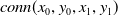
Running Example. As an example of a classical planning problem, we can model the navigation task shown in Figure 1 as follows. Let n and m be the boundaries of our grid. One can use n objects to represent x-coordinates and m objects for the y-coordinates. Then, predicate at(x,y) models whether the agent is in position (x,y); predicate
 $conn(x_0,y_0,x_1,y_1)$
models whether the two cells
$conn(x_0,y_0,x_1,y_1)$
models whether the two cells
 $(x_0,y_0)$
and
$(x_0,y_0)$
and
 $(x_1,y_1)$
are connected or not. Given all these predicates, we can build an operator
$(x_1,y_1)$
are connected or not. Given all these predicates, we can build an operator
 $move(x_0,y_0,x_1,y_1)$
that models the movement from a cell to another. The precondition of the operator simultaneously ensures that
$move(x_0,y_0,x_1,y_1)$
that models the movement from a cell to another. The precondition of the operator simultaneously ensures that
 $conn(x_0,y_0,x_1,y_1)$
and
$conn(x_0,y_0,x_1,y_1)$
and
 $at(x_0,y_0)$
are true; the effect instead models that
$at(x_0,y_0)$
are true; the effect instead models that
 $at(x_0,y_0)$
will be false at the end of the execution, and that
$at(x_0,y_0)$
will be false at the end of the execution, and that
 $at(x_1,y_1)$
will instead be true. The initial state and the goals are also quite trivial. The initial state contains as many facts as connections in the grid (the obstacles are implicit), and a fact representing the initial position of the agent. As a goal we simply require the agent to be in the position where the key is. For the grid in Figure 1(a), this can be represented by having
$at(x_1,y_1)$
will instead be true. The initial state and the goals are also quite trivial. The initial state contains as many facts as connections in the grid (the obstacles are implicit), and a fact representing the initial position of the agent. As a goal we simply require the agent to be in the position where the key is. For the grid in Figure 1(a), this can be represented by having
 $\{at(4,0)\} \subset I$
and
$\{at(4,0)\} \subset I$
and
 $G = \{at(0,3)\}$
. Note that here we use numbers for objects for convenience, while they are treated just as strings. A plan
$G = \{at(0,3)\}$
. Note that here we use numbers for objects for convenience, while they are treated just as strings. A plan
 $\pi_1$
solving such a task is the sequence
$\pi_1$
solving such a task is the sequence
 $\langle move(4,0,3,0),$
move(3, 0, 3, 1), move(3, 1, 3, 2), move(3, 2, 2, 2), move(2, 2, 1, 2), move(1, 2, 0, 2),
$\langle move(4,0,3,0),$
move(3, 0, 3, 1), move(3, 1, 3, 2), move(3, 2, 2, 2), move(2, 2, 1, 2), move(1, 2, 0, 2),
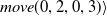 $move(0,2,0,3) \rangle$
, represented by the red arrows in the grid of Figure 1(a). For the problem depicted in Figure 1(b),
$move(0,2,0,3) \rangle$
, represented by the red arrows in the grid of Figure 1(a). For the problem depicted in Figure 1(b),
 $\{at(3,0)\} \subset I$
and the goal G is the same as for Figure 1(a). A plan
$\{at(3,0)\} \subset I$
and the goal G is the same as for Figure 1(a). A plan
 $\pi_2$
solving such a task is the sequence
$\pi_2$
solving such a task is the sequence
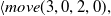 $\langle move(3,0,2,0),$
move(2, 0, 1, 0), move(1, 0, 0, 0), move(0, 0, 0, 1), move(0, 1, 0, 2),
$\langle move(3,0,2,0),$
move(2, 0, 1, 0), move(1, 0, 0, 0), move(0, 0, 0, 1), move(0, 1, 0, 2),
 $\pi_1^{7,7}\rangle$
, represented by the blue arrows and a red arrow in the grid of Figure 1(b). Of course, there might exist more than one plan solving a planning problem. Another solution is a plan,
$\pi_1^{7,7}\rangle$
, represented by the blue arrows and a red arrow in the grid of Figure 1(b). Of course, there might exist more than one plan solving a planning problem. Another solution is a plan,
 $\pi_3$
, consisting of
$\pi_3$
, consisting of
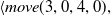 $\langle move(3,0,4,0),$
move(4, 0, 4, 1), move(4, 1, 4, 2), move(4, 2, 3, 2),
$\langle move(3,0,4,0),$
move(4, 0, 4, 1), move(4, 1, 4, 2), move(4, 2, 3, 2),
 $\pi_2^{4,7} \rangle$
, represented by the green arrows and the red arrows in the grid of Figure 1(b).
$\pi_2^{4,7} \rangle$
, represented by the green arrows and the red arrows in the grid of Figure 1(b).
3. The repair planning problem
A repair planning problem combines a planning problem and a plan attempting to solve such a problem. We formally define a repair planning problem as follows.
Definition 1 (Repair problem). A repair planning problem is the pair
 $ \langle {{{\mathcal{P}}}},\pi\rangle $
, where
$ \langle {{{\mathcal{P}}}},\pi\rangle $
, where
 $ {{{\mathcal{P}}}} $
is a planning problem and
$ {{{\mathcal{P}}}} $
is a planning problem and
 $ \pi $
is some sequence of actions from actions in
$ \pi $
is some sequence of actions from actions in
 $ {{{\mathcal{P}}}} $
.
$ {{{\mathcal{P}}}} $
.
A plan solves the repair problem if and only if it solves
 $ {{{\mathcal{P}}}} $
, too. What differs from the planning problem is the notion of optimality.
$ {{{\mathcal{P}}}} $
, too. What differs from the planning problem is the notion of optimality.
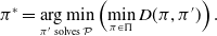
Definition 2 (Optimal plan repair). A plan
 $\pi^*$
is said to be optimal for a repair problem
$\pi^*$
is said to be optimal for a repair problem
 $ \langle {{{\mathcal{P}}}},\pi\rangle $
if it is the one that minimizes the distance from the input plan
$ \langle {{{\mathcal{P}}}},\pi\rangle $
if it is the one that minimizes the distance from the input plan
 $ \pi $
and solves
$ \pi $
and solves
 $ {{{\mathcal{P}}}} $
. Formally, let
$ {{{\mathcal{P}}}} $
. Formally, let
 $D\;:\; \hat{\Pi}_{{{\mathcal{P}}}} \times \hat{\Pi}_{{{\mathcal{P}}}} \rightarrow \mathbb{R}$
be a function measuring the distance between two plans for problem
$D\;:\; \hat{\Pi}_{{{\mathcal{P}}}} \times \hat{\Pi}_{{{\mathcal{P}}}} \rightarrow \mathbb{R}$
be a function measuring the distance between two plans for problem
 ${{{\mathcal{P}}}}$
. Then:
${{{\mathcal{P}}}}$
. Then:
 \[\pi^* = \mathop{\operatorname{arg\,min}}_{\pi' \text{ solves } {{{\mathcal{P}}}}}D(\pi,\pi').\]
Intuitively, given the input plan
 $\pi$
and any solution of the replair planning problem we are looking for the most similar plan, and do so by characterizing the distance between any two plans by the function D which is defined in the next paragraph. The input plan
$\pi$
and any solution of the replair planning problem we are looking for the most similar plan, and do so by characterizing the distance between any two plans by the function D which is defined in the next paragraph. The input plan
 $\pi$
might be a plan that was already used and validated by humans and, as mentioned before, finding a solution plan that is similar to
$\pi$
might be a plan that was already used and validated by humans and, as mentioned before, finding a solution plan that is similar to
 $\pi$
would guarantee coherence and consistency with already used behaviors and would reduce the cognitive load on humans.
$\pi$
would guarantee coherence and consistency with already used behaviors and would reduce the cognitive load on humans.
In this work, we use a simple notion of plan distance, which considers a plan more stable if it is closer to the input plan in terms of number of different actions they contain, while we ignore the action ordering in plans. This is the same notion of plan distance proposed by Fox et al. (Reference Fox, Gerevini, Long and Serina2006). Let
 $\pi $
and
$\pi $
and
 $ \pi' $
be two plans. For the definition of plan distance, we treat
$ \pi' $
be two plans. For the definition of plan distance, we treat
 $\pi $
and
$\pi $
and
 $ \pi' $
as multisets of actions. We use multisets rather than simple action sets because a plan may contain multiple instances of the same action. Formally, the distance D between
$ \pi' $
as multisets of actions. We use multisets rather than simple action sets because a plan may contain multiple instances of the same action. Formally, the distance D between
 $ \pi $
and
$ \pi $
and
 $ \pi' $
is defined as
$ \pi' $
is defined as
 \begin{equation}D(\pi,\pi') = | \pi \setminus \pi' | + | \pi' \setminus \pi |\end{equation}
Note here that we are operating over multisets, that is, repetition of the same action does matter. For this reason, operator
 $\setminus$
is defined so that
$\setminus$
is defined so that
 $\pi\!\setminus\!\pi'$
contains
$\pi\!\setminus\!\pi'$
contains
 $m-l$
instances of action a iff
$m-l$
instances of action a iff
 $\pi$
and
$\pi$
and
 $\pi'$
, respectively, contain m and l instances of a and
$\pi'$
, respectively, contain m and l instances of a and
 $m \gt l$
;
$m \gt l$
;
 $\pi\!\setminus\!\pi'$
contains 0 instances of a otherwise. The smaller the distance between the new plan and the input plan, the more stable the new plan is with respect to the input plan.
$\pi\!\setminus\!\pi'$
contains 0 instances of a otherwise. The smaller the distance between the new plan and the input plan, the more stable the new plan is with respect to the input plan.
Running Example (cont.) As for the plans depicted in Figure 1, let
 $\pi_1$
be the plan represented by the red arrows in the grid of Figure 1(a);
$\pi_1$
be the plan represented by the red arrows in the grid of Figure 1(a);
 $\pi_2$
be the plan represented by the blue arrows and a red arrow in the grid of Figure 1(b);
$\pi_2$
be the plan represented by the blue arrows and a red arrow in the grid of Figure 1(b);
 $\pi_3$
be the plan represented by the green and red arrows in the grid of Figure 1(b). The distance between
$\pi_3$
be the plan represented by the green and red arrows in the grid of Figure 1(b). The distance between
 $\pi_1$
and
$\pi_1$
and
 $\pi_2$
is 11, the sum between 5 and 6, because the 5 actions in
$\pi_2$
is 11, the sum between 5 and 6, because the 5 actions in
 $\pi_2^{1,5}$
are not in
$\pi_2^{1,5}$
are not in
 $\pi_1$
(the blue arrows in the figure), and the 6 actions in
$\pi_1$
(the blue arrows in the figure), and the 6 actions in
 $\pi_1^{1,6}$
are not in
$\pi_1^{1,6}$
are not in
 $\pi_2$
. The distance between
$\pi_2$
. The distance between
 $\pi_1$
and
$\pi_1$
and
 $\pi_3$
is 7, the sum between 4 and 3, because the 4 actions in
$\pi_3$
is 7, the sum between 4 and 3, because the 4 actions in
 $\pi_3^{1,4}$
are not in
$\pi_3^{1,4}$
are not in
 $\pi_1$
(the green arrows in the figure), and the 3 actions in
$\pi_1$
(the green arrows in the figure), and the 3 actions in
 $\pi_1^{1,3}$
are not in
$\pi_1^{1,3}$
are not in
 $\pi_3$
. Consider the repair planning problem defined as the grid-based navigation problem instance depicted in Figure 1(b) and plan
$\pi_3$
. Consider the repair planning problem defined as the grid-based navigation problem instance depicted in Figure 1(b) and plan
 $\pi_1$
. Plan
$\pi_1$
. Plan
 $\pi_3$
is the optimal repair plan for this instance of the problem because there exists no plan with a distance from
$\pi_3$
is the optimal repair plan for this instance of the problem because there exists no plan with a distance from
 $\pi_1$
lower than the distance between
$\pi_1$
lower than the distance between
 $\pi_3$
and
$\pi_3$
and
 $\pi_1$
.
$\pi_1$
.
In general, there might be more than one plan that were already successfully used to solve problems similar to the new encountered planning problem
 ${{{\mathcal{P}}}}$
. Thereby, the goal of ensuring coherence and consistency with already used behaviors is achieved if the solution of the new encountered problem is similar to any already successfully used plan. For this reason, we define an extension of the repair planning problem that combines a planning problem and a set of input plans.
${{{\mathcal{P}}}}$
. Thereby, the goal of ensuring coherence and consistency with already used behaviors is achieved if the solution of the new encountered problem is similar to any already successfully used plan. For this reason, we define an extension of the repair planning problem that combines a planning problem and a set of input plans.
Definition 3 (Multi-repair planning problem). A multi-repair planning problem is the pair
 $ \langle {{{\mathcal{P}}}},\Pi\rangle $
, where
$ \langle {{{\mathcal{P}}}},\Pi\rangle $
, where
 $ {{{\mathcal{P}}}} $
is a planning problem and
$ {{{\mathcal{P}}}} $
is a planning problem and
 $ \Pi \subseteq \hat{\Pi}_{{{\mathcal{P}}}}$
is a set of plans for
$ \Pi \subseteq \hat{\Pi}_{{{\mathcal{P}}}}$
is a set of plans for
 ${{{\mathcal{P}}}}$
, each of which is some sequence of actions from actions in
${{{\mathcal{P}}}}$
, each of which is some sequence of actions from actions in
 $ {{{\mathcal{P}}}} $
.
$ {{{\mathcal{P}}}} $
.
Like for the single repair planning problem, we say that a plan solves the multi-repair planning problem if and only if it solves
 ${{{\mathcal{P}}}}$
. Differently from the single repair problem, the notion of optimality for the multi-repair planning problem takes into account all the input plans in the problem definition.
${{{\mathcal{P}}}}$
. Differently from the single repair problem, the notion of optimality for the multi-repair planning problem takes into account all the input plans in the problem definition.
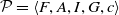
Definition 4 (Optimal multi-repair plan). A plan is said to be optimal for a multi-repair problem if it is the one that minimizes the distance from any input plan
 $ \pi \in \Pi$
and solves
$ \pi \in \Pi$
and solves
 $ {{{\mathcal{P}}}} $
. Formally, let
$ {{{\mathcal{P}}}} $
. Formally, let
 $D\;:\; \hat{\Pi}_{{{\mathcal{P}}}} \times \hat{\Pi}_{{{\mathcal{P}}}} \rightarrow \mathbb{R}$
be a function measuring the distance between two plans for problem
$D\;:\; \hat{\Pi}_{{{\mathcal{P}}}} \times \hat{\Pi}_{{{\mathcal{P}}}} \rightarrow \mathbb{R}$
be a function measuring the distance between two plans for problem
 ${{{\mathcal{P}}}}$
. Then:
${{{\mathcal{P}}}}$
. Then:
 \[\pi^* = \mathop{\operatorname{arg\,min}}_{\pi' \text{ solves } {{{\mathcal{P}}}}} \left(\min_{\pi \in \Pi} D(\pi,\pi')\right).\]
4. Solving the optimal repairing problem
This section presents a compilation that takes in input a repair problem and generates a novel classical problem whose optimal solutions are optimal solutions for the repair planning problem. Our compilation creates a number of copies for each action in the plan and customises the cost function for keeping track of those actions undermining the optimality of the solution. The compilation also makes use of a number of additional, dummy predicates, whose purpose is to monitor the already executed actions. Specifically, the new set of predicates, denoted F ′, extends the original set F with
-
• a dummy atom w, whose truth value distinguishes two stages: the first stage constructs the solution, while the second stage evaluates its quality;
-
• a set of predicates that serve as proxies for the actions in the input plan, and
-
• a set of predicates that, for each action in the input plan, track the number of times that action has already been executed in the new plan.
The new initial state, I ′, extends the original initial state I by including w, indicating that the planner starts at the first stage, and by adding special atoms that specify, for each action a in the input plan, that zero occurrences of a have been executed initially. The new set of actions, A ′, is divided into four subsets:
-
•
 $A_0$
, action instances that appear in the input plan,
$A_0$
, action instances that appear in the input plan, -
•
$A_1$
, actions not present in the input plan, -
•
$A_2$
, actions from the input plan that have already been used in the new plan, and -
•
$A_3$
, action instances from the input plan that are not considered for the new plan.


The new goal state, G ′, extends the original goal set by adding literals that force the planner to either include the actions of the input plan in the new plan or account for them when defining the plan cost. Finally, the compilation scheme defines a cost function c ′ that encourages the use of actions from the input plan, while discouraging the use of actions not in the input plan, the omission of input-plan actions, as well as an excessive reuse of input-plan actions. In this compilation, we work at the grounding level. That is, we assume that all actions have been instantiated against the objects of our problem. Grounding can be achieved using well-known reachability based techniques (Helmert, Reference Helmert2006). Then, in the next section, we also show a compilation that does not require grounding upfront.
In what follows, we formally explain the grounded compilation, that we call Resa (REpair for StAbility). We use two functions to simplify notation. Function
 $ B(a,i,\pi) $
counts the number of occurrences of input action a Before step i in plan
$ B(a,i,\pi) $
counts the number of occurrences of input action a Before step i in plan
 $\pi$
; formally,
$\pi$
; formally,
 $ B \;:\; A \times \mathbb{N} \times 2^{A^*}\rightarrow \mathbb{N}$
. Function
$ B \;:\; A \times \mathbb{N} \times 2^{A^*}\rightarrow \mathbb{N}$
. Function
 $ M \;:\; A \times 2^{A^*} \rightarrow \mathbb{N} $
returns the number of repetitions of an action in a plan.
$ M \;:\; A \times 2^{A^*} \rightarrow \mathbb{N} $
returns the number of repetitions of an action in a plan.
Definition 5 (Resa Compilation). Let
 $ {{{\mathcal{P}}}} = \langle F, A, I, G, c \rangle$
be a planning problem, and
$ {{{\mathcal{P}}}} = \langle F, A, I, G, c \rangle$
be a planning problem, and
 $ \pi = \langle a_1,\dots,a_n \rangle $
be a sequence of n actions in A. Resa takes in input
$ \pi = \langle a_1,\dots,a_n \rangle $
be a sequence of n actions in A. Resa takes in input
 $ {{{\mathcal{P}}}} $
and
$ {{{\mathcal{P}}}} $
and
 $ \pi $
, and generates a new planning problem
$ \pi $
, and generates a new planning problem
 $ {{{\mathcal{P}}}}' = \langle F', A_0 \cup A_1 \cup A_2 \cup A_3 \cup \{switch\}, I', G', c' \rangle$
such that:
$ {{{\mathcal{P}}}}' = \langle F', A_0 \cup A_1 \cup A_2 \cup A_3 \cup \{switch\}, I', G', c' \rangle$
such that:
 \begin{align*} F' = \;& F \cup \{w\} \cup \bigcup_{ i\in \{1,\dots,n \} }{d_i} \cup \bigcup_{a \in \pi} \{ p^{i}_{a} \mid 0 \le i \le M(a,\pi)\}\\ I' =\; & I \cup \{w\}\cup \bigcup_{a \in \pi}p_{a}^0\\ A_{0} =\; & \bigcup_{a_i \in \pi} \langle \mathsf{pre}(a)\land w\land p^{{{{B(a,i,\pi)}}}}_{a}, \mathsf{eff}(a) \cup \{ p^{{{{B(a,i,\pi)}}}+1}_{a},\neg p^{{{{B(a,i,\pi)}}}}_{a},{{{d}}}_i\} \rangle\\ A_{1} = & \bigcup_{a \in A \setminus set(\pi)} \langle \mathsf{pre}(a)\land w, \mathsf{eff}(a) \rangle\\ A_{2} = & \bigcup_{a \in set(\pi)} \langle \mathsf{pre}(a)\land w \land p^{{{{M(a,\pi)}}}}_{a}, \mathsf{eff}(a) \rangle\\A_{3} = & \bigcup_{ i\in \{1,\dots,n \} }\langle \neg w \land \neg {{{d}}}_i, \{{{{d}}}_i\} \rangle\\ switch =\; & \langle w,\{\neg w\} \rangle\\ G' =\; & G \land \bigwedge_{ i\in \{1,\dots,n \} }{{{d}}}_i\\ c'(a) = & \begin{cases} 0 & \operatorname{if } a \in A_0 \cup \{switch\}\\ 1 & \operatorname{if } a \in A_1 \cup A_2 \cup A_3 \end{cases}\end{align*}
Intuitively, the compilation reshapes the planning problem in such a way that all actions that do not contribute in increasing the distance from the previous plan are given cost 0. Action instances that instead were not in the plan (the actions set
 $ A_1 $
) or that were in the plan but we have already used them (set
$ A_1 $
) or that were in the plan but we have already used them (set
 $ A_2 $
), or that were in the plan but are not going to be considered for the new plan (set
$ A_2 $
), or that were in the plan but are not going to be considered for the new plan (set
 $ A_3 $
) are given cost 1. Indeed, the goal formula requires that, besides achieving the problem goals, all actions of the input plan are processed. This is achieved by formulating a fact d for each action within the starting plan. Such a fact can either be made true by actions from set
$ A_3 $
) are given cost 1. Indeed, the goal formula requires that, besides achieving the problem goals, all actions of the input plan are processed. This is achieved by formulating a fact d for each action within the starting plan. Such a fact can either be made true by actions from set
 $ A_0 $
whose cost is equal to 0 – indeed that corresponds to the case in which we did replicate what the plan was before, or actions from
$ A_0 $
whose cost is equal to 0 – indeed that corresponds to the case in which we did replicate what the plan was before, or actions from
 $ A_3 $
whose cost is equal to 1. Basically, actions from
$ A_3 $
whose cost is equal to 1. Basically, actions from
 $ A_3 $
are the give-up actions, that is, they emulate whether the planner gave up in trying to pick actions from the input plan and for that it pays an extra cost of 1 for each one of them. These dummy actions share some analogy with previous work to compile soft goals away (Keyder & Geffner, Reference Keyder and Geffner2009).
$ A_3 $
are the give-up actions, that is, they emulate whether the planner gave up in trying to pick actions from the input plan and for that it pays an extra cost of 1 for each one of them. These dummy actions share some analogy with previous work to compile soft goals away (Keyder & Geffner, Reference Keyder and Geffner2009).
In order to consider whether some action instance has been already considered we make use of the aforementioned functions B and M. These functions make it possible to create as many
 $ p_a $
predicates as needed to keep track of the number of instances of used action a, and to monitor whether limit
$ p_a $
predicates as needed to keep track of the number of instances of used action a, and to monitor whether limit
 $ M(a,\pi) $
has been hit. The initial state contains an atom
$ M(a,\pi) $
has been hit. The initial state contains an atom
 $p_a^0$
for each action a used in the input plan. As mentioned above, this special atom indicates that the number of occurrences of action a contained in the (partial) plan under construction is initially zero. The first instance of action a added to the partial plan is an action in
$p_a^0$
for each action a used in the input plan. As mentioned above, this special atom indicates that the number of occurrences of action a contained in the (partial) plan under construction is initially zero. The first instance of action a added to the partial plan is an action in
 $A_0$
that makes
$A_0$
that makes
 $p_a^0$
false while achieves
$p_a^0$
false while achieves
 $p_a^1$
. In general, atom
$p_a^1$
. In general, atom
 $p_a^i$
represents the fact that the number of occurrences of action a in the plan under construction is i. The last instance of action a that is part of set
$p_a^i$
represents the fact that the number of occurrences of action a in the plan under construction is i. The last instance of action a that is part of set
 $A_0$
and is added to the plan under construction makes
$A_0$
and is added to the plan under construction makes
 $p_a^{M(a,\pi)}$
true. This means that all the occurrences of action a in the input plan have been added to the plan under construction. This way, precondition
$p_a^{M(a,\pi)}$
true. This means that all the occurrences of action a in the input plan have been added to the plan under construction. This way, precondition
 $p_a^{M(a,\pi)}$
of the copy of action a in set
$p_a^{M(a,\pi)}$
of the copy of action a in set
 $A_2$
is true, any extra occurrence of action a that will be eventually added to the plan under construction will be such an action copy of a in
$A_2$
is true, any extra occurrence of action a that will be eventually added to the plan under construction will be such an action copy of a in
 $A_2$
and will increase the distance from the starting plan. The switch action is what marks the end of the first stage and the beginning of the second, finalizing the search of the plan and starting the collection of the give-up actions from
$A_2$
and will increase the distance from the starting plan. The switch action is what marks the end of the first stage and the beginning of the second, finalizing the search of the plan and starting the collection of the give-up actions from
 $ A_3 $
. Indeed, none of the actions is executable after switch but those in
$ A_3 $
. Indeed, none of the actions is executable after switch but those in
 $ A_3$
. This is guaranteed by dummy literal w, which is true in the initial state, required by any action in sets
$ A_3$
. This is guaranteed by dummy literal w, which is true in the initial state, required by any action in sets
 $A_0$
,
$A_0$
,
 $A_1$
, and
$A_1$
, and
 $A_2$
, and made false by action switch; in addition, any action in set
$A_2$
, and made false by action switch; in addition, any action in set
 $A_3$
requires that w is false.
$A_3$
requires that w is false.
Running Example (cont.) In order to see how the compilation works in practice, let us take a look at our grid-based navigation example. Consider the repair planning problem defined as the grid-based navigation problem instance depicted in Figure 1(b), and the input plan defined as the plan represented by the red arrows in the grid of Figure 1(a). First, we augment the set of predicates to include those representing the various action instances. Therefore, we define
 $F' = F \cup \{d_1,\cdots,d_{7}\} \cup \{w\} \cup \bigcup_{i \in \{0,1\}} \{p^{i}_{m_{4,0,3,0}},p^{i}_{m_{3,0,3,1}},p^{i}_{m_{3,1,3,2}},p^{i}_{m_{3,2,2,2}},p^{i}_{m_{2,2,2,1}},p^{i}_{m_{2,1,2,0}},p^{i}_{m_{2,0,3,0}}\}$
. Here, the subscripts denote the names of the move actions as introduced earlier, with parameters written as subscripts for clarity. The initial state is updated to include the switch phase predicate w, and the predicates indicating that the number of occurrences of the actions in the input plan is initially zero in the plan under construction. That is, we define
$F' = F \cup \{d_1,\cdots,d_{7}\} \cup \{w\} \cup \bigcup_{i \in \{0,1\}} \{p^{i}_{m_{4,0,3,0}},p^{i}_{m_{3,0,3,1}},p^{i}_{m_{3,1,3,2}},p^{i}_{m_{3,2,2,2}},p^{i}_{m_{2,2,2,1}},p^{i}_{m_{2,1,2,0}},p^{i}_{m_{2,0,3,0}}\}$
. Here, the subscripts denote the names of the move actions as introduced earlier, with parameters written as subscripts for clarity. The initial state is updated to include the switch phase predicate w, and the predicates indicating that the number of occurrences of the actions in the input plan is initially zero in the plan under construction. That is, we define
 $I' = I \cup \{w\} \cup \{p^{0}_{m_{4,0,3,0}},p^{0}_{m_{3,0,3,1}},p^{0}_{m_{3,1,3,2}},p^{0}_{m_{3,2,2,2}},p^{0}_{m_{2,2,2,1}},p^{0}_{m_{2,1,2,0}},p^{0}_{m_{2,0,3,0}}\}$
. In this plan, there is only one instance of each action, that is,
$I' = I \cup \{w\} \cup \{p^{0}_{m_{4,0,3,0}},p^{0}_{m_{3,0,3,1}},p^{0}_{m_{3,1,3,2}},p^{0}_{m_{3,2,2,2}},p^{0}_{m_{2,2,2,1}},p^{0}_{m_{2,1,2,0}},p^{0}_{m_{2,0,3,0}}\}$
. In this plan, there is only one instance of each action, that is,
 $M(a,\pi) = 1\;\; \forall a \in \pi$
, so function B will only be used to differentiate whether the action has been used or not—and this is also the reason why we have only two predicates per action.
$M(a,\pi) = 1\;\; \forall a \in \pi$
, so function B will only be used to differentiate whether the action has been used or not—and this is also the reason why we have only two predicates per action.
For simplicity, we will now consider the encoding of two actions move(3, 1, 3, 2) and move(2, 1, 3, 2), symbolically denoted as
 $a = {m_{3,1,3,2}}$
and
$a = {m_{3,1,3,2}}$
and
 $b = {m_{2,1,3,2}}$
. Action a is in the input plan, while b is not part of such a plan. For action a, we create an instance in set
$b = {m_{2,1,3,2}}$
. Action a is in the input plan, while b is not part of such a plan. For action a, we create an instance in set
 $A_0$
with the conjunction between the precondition formula of a and atom
$A_0$
with the conjunction between the precondition formula of a and atom
 $p^{0}_{m_{3,1,3,2}}$
as precondition, and the set of effects of a extended by atoms
$p^{0}_{m_{3,1,3,2}}$
as precondition, and the set of effects of a extended by atoms
 $\neg p^{0}_{m_{3,1,3,2}}$
,
$\neg p^{0}_{m_{3,1,3,2}}$
,
 $ p^{1}_{m_{3,1,3,2}}$
, and
$ p^{1}_{m_{3,1,3,2}}$
, and
 $ d_3 $
as set of effects. Atom
$ d_3 $
as set of effects. Atom
 $d_3$
in the set of effects of a indicates that, when action a is executed, the third action in the input plan is included into the plan under construction. Additionally, we need a copy of a, labeled a ′, which belongs to set
$d_3$
in the set of effects of a indicates that, when action a is executed, the third action in the input plan is included into the plan under construction. Additionally, we need a copy of a, labeled a ′, which belongs to set
 $A_2$
, where
$A_2$
, where
 $\mathsf{pre}(a') = \mathsf{pre}(a) \wedge w \wedge p^{1}_{m_{3,1,3,2}} \quad \text{and} \quad \mathsf{eff}(a') = \mathsf{eff}(a)$
. Another difference between these two instances is the cost: the interpretation in
$\mathsf{pre}(a') = \mathsf{pre}(a) \wedge w \wedge p^{1}_{m_{3,1,3,2}} \quad \text{and} \quad \mathsf{eff}(a') = \mathsf{eff}(a)$
. Another difference between these two instances is the cost: the interpretation in
 $A_0$
has a cost of 0 (as it reuses part of the previous plan), while the interpretation in
$A_0$
has a cost of 0 (as it reuses part of the previous plan), while the interpretation in
 $A_2$
has a cost of 1, representing the extra cost of executing the action a number of times greater than in the input plan.
$A_2$
has a cost of 1, representing the extra cost of executing the action a number of times greater than in the input plan.
For action b, which is not part of the plan, we need only one interpretation, stored in set
 $A_1$
. Such an instance is the same as b but its cost is 1 and w is part of its precondition formula. Indeed, this action must be executed before the predicate w becomes false, as w tracks whether the plan is complete and when the cost of the repair should be calculated.
$A_1$
. Such an instance is the same as b but its cost is 1 and w is part of its precondition formula. Indeed, this action must be executed before the predicate w becomes false, as w tracks whether the plan is complete and when the cost of the repair should be calculated.
Finally, set
 $A_3$
for this problem consists of 7 actions, one for each instance of each action in the plan. That is:
$A_3$
for this problem consists of 7 actions, one for each instance of each action in the plan. That is:
 $A_3 = \{\langle \neg w \wedge \neg d_1, d_1 \rangle, \cdots, \langle \neg w \wedge \neg d_7, d_7 \rangle\}$
. The actions in
$A_3 = \{\langle \neg w \wedge \neg d_1, d_1 \rangle, \cdots, \langle \neg w \wedge \neg d_7, d_7 \rangle\}$
. The actions in
 $A_3$
have cost equal to 1, because each of them represents the absence of an action of the input plan from the solution for the repair planning problem. The formulation of the goal is straightforward. Indeed, what we would only need is to conjoin the goal formula G with all atoms
$A_3$
have cost equal to 1, because each of them represents the absence of an action of the input plan from the solution for the repair planning problem. The formulation of the goal is straightforward. Indeed, what we would only need is to conjoin the goal formula G with all atoms
 $d_i$
. This way we know for sure that either we used an action instance from the plan or we add some cost for its absence.
$d_i$
. This way we know for sure that either we used an action instance from the plan or we add some cost for its absence.
4.1. Properties of Resa
In this section, we study some properties of Resa. In particular, we prove that Resa is sound, complete and always generates optimal solutions for the repair problem it is encoding. Moreover, Resa size is polynomial in the input task.
Theorem 1 (Soundness). Let
 $ {{{\mathcal{R}}}} = \langle {{{\mathcal{P}}}}, \pi \rangle $
be a plan repair problem. Resa transforms
$ {{{\mathcal{R}}}} = \langle {{{\mathcal{P}}}}, \pi \rangle $
be a plan repair problem. Resa transforms
 $ {{{\mathcal{R}}}} $
into a problem
$ {{{\mathcal{R}}}} $
into a problem
 $ {{{\mathcal{P}}}}' $
such that if
$ {{{\mathcal{P}}}}' $
such that if
 $ {{{\mathcal{P}}}}' $
is solvable so is
$ {{{\mathcal{P}}}}' $
is solvable so is
 $ {{{\mathcal{R}}}} $
.
$ {{{\mathcal{R}}}} $
.
Proof. Each plan computed by Resa has one of the following two forms, for
 $k \geq 0, m\geq 0$
:
$k \geq 0, m\geq 0$
:
 \begin{align*} \begin{array}{ll} & \langle \underbrace{a_1, \dots, a_k}_{\pi'}\rangle,\\ & \langle \underbrace{a_1, \dots, a_k}_{\pi'}, switch, \underbrace{a_{k+1}, \dots, a_m}_{\pi''} \rangle \nonumber \end{array} \end{align*}
The Resa plan has the same form as the first plan if all the occurrences of the actions in the input plan are in
 $\pi'$
, has the latter form otherwise. Each action in the first part of the plan,
$\pi'$
, has the latter form otherwise. Each action in the first part of the plan,
 $\pi'$
, is in sets
$\pi'$
, is in sets
 $A_0$
,
$A_0$
,
 $A_1$
, or
$A_1$
, or
 $A_2$
, since actions in
$A_2$
, since actions in
 $A_3$
has
$A_3$
has
 $\neg w$
as precondition, w is true in the initial state, and the only action that made w false is switch. Similarly, each action in the second part of the plan,
$\neg w$
as precondition, w is true in the initial state, and the only action that made w false is switch. Similarly, each action in the second part of the plan,
 $\pi''$
, is in set
$\pi''$
, is in set
 $A_3$
, since every other action has w as precondition and w becomes false after the execution of the switch action. For construction, each action in
$A_3$
, since every other action has w as precondition and w becomes false after the execution of the switch action. For construction, each action in
 $A_0$
,
$A_0$
,
 $A_1$
, or
$A_1$
, or
 $A_2$
has the same preconditions and effects in set F as an action of
$A_2$
has the same preconditions and effects in set F as an action of
 ${{{\mathcal{P}}}}$
, plus some additional preconditions and effects in
${{{\mathcal{P}}}}$
, plus some additional preconditions and effects in
 $F'\!\setminus\!F$
. In practice, all such actions require the preconditions of the original actions to hold before their execution, and the original effects are preserved; the remaining preconditions and effects only monitor whether the action instance is playing the role of an action that was in the input plan, or not. The goal of
$F'\!\setminus\!F$
. In practice, all such actions require the preconditions of the original actions to hold before their execution, and the original effects are preserved; the remaining preconditions and effects only monitor whether the action instance is playing the role of an action that was in the input plan, or not. The goal of
 ${{{\mathcal{P}}}}'$
that are in F are the same as in
${{{\mathcal{P}}}}'$
that are in F are the same as in
 ${{{\mathcal{P}}}}$
. Action switch and the action in
${{{\mathcal{P}}}}$
. Action switch and the action in
 $\pi''$
do not change the truth value of facts in F, therefore the goals in F are achieved at the end of
$\pi''$
do not change the truth value of facts in F, therefore the goals in F are achieved at the end of
 $\pi'$
. It follows that the sequence of original actions from which we derived the action in
$\pi'$
. It follows that the sequence of original actions from which we derived the action in
 $\pi'$
is a plan solving
$\pi'$
is a plan solving
 ${{{\mathcal{P}}}}$
.
${{{\mathcal{P}}}}$
.
Theorem 2 (Completeness). Let
 $ {{{\mathcal{R}}}} = \langle {{{\mathcal{P}}}}, \pi \rangle $
be a plan repair problem. Resa transforms
$ {{{\mathcal{R}}}} = \langle {{{\mathcal{P}}}}, \pi \rangle $
be a plan repair problem. Resa transforms
 $ {{{\mathcal{R}}}} $
into a problem
$ {{{\mathcal{R}}}} $
into a problem
 $ {{{\mathcal{P}}}}' $
that is solvable if
$ {{{\mathcal{P}}}}' $
that is solvable if
 ${{{\mathcal{R}}}}$
is solvable.
${{{\mathcal{R}}}}$
is solvable.
Proof. For any valid plan
 $ \pi_1 = \langle a_1, \dots, a_m \rangle$
of
$ \pi_1 = \langle a_1, \dots, a_m \rangle$
of
 ${{{\mathcal{R}}}}$
there is (at least) one plan
${{{\mathcal{R}}}}$
there is (at least) one plan
 $\pi_2$
in the compiled problem
$\pi_2$
in the compiled problem
 $ {{{\mathcal{P}}}}' $
which can be constructed as follows. Plan
$ {{{\mathcal{P}}}}' $
which can be constructed as follows. Plan
 $\pi_2$
has the first m actions that are copies of actions in
$\pi_2$
has the first m actions that are copies of actions in
 $\pi_1$
from set
$\pi_1$
from set
 $ A_0 $
,
$ A_0 $
,
 $ A_1 $
, or
$ A_1 $
, or
 $ A_2 $
. We show that the j-th action of
$ A_2 $
. We show that the j-th action of
 $\pi_2$
is applicable in
$\pi_2$
is applicable in
 $\pi_2^{1,j-1}[I']$
for
$\pi_2^{1,j-1}[I']$
for
 $1 \le j \le m$
. For each action a in
$1 \le j \le m$
. For each action a in
 $\pi_1$
, we distinguish three cases: (i) a is an instance of an action that is not part of the input plan; (ii) a is an instance of an action that has k occurrences in the input plan, is the i-th occurrence of the action in
$\pi_1$
, we distinguish three cases: (i) a is an instance of an action that is not part of the input plan; (ii) a is an instance of an action that has k occurrences in the input plan, is the i-th occurrence of the action in
 $\pi_1$
and
$\pi_1$
and
 $i \le k$
; (iii) a is an instance of an action that has k occurrences in the input plan, is the i-th occurrence of the action in
$i \le k$
; (iii) a is an instance of an action that has k occurrences in the input plan, is the i-th occurrence of the action in
 $\pi_1$
and
$\pi_1$
and
 $i \gt k$
. Let a be the j-th action in
$i \gt k$
. Let a be the j-th action in
 $\pi_1$
. For case (i), a has a copy in set
$\pi_1$
. For case (i), a has a copy in set
 $A_1$
that is applicable in
$A_1$
that is applicable in
 $\pi_2^{1,j-1}[I']$
because the action preconditions and effects that are in F are the same as in
$\pi_2^{1,j-1}[I']$
because the action preconditions and effects that are in F are the same as in
 ${{{\mathcal{R}}}}$
. The only difference between a and its copy is that the copy has w as a precondition. Such a precondition is true in the state where the a’s copy is executed, because w is true in the initial state and the copies of the actions in
${{{\mathcal{R}}}}$
. The only difference between a and its copy is that the copy has w as a precondition. Such a precondition is true in the state where the a’s copy is executed, because w is true in the initial state and the copies of the actions in
 $\pi_2$
executed before the copy of a are in sets
$\pi_2$
executed before the copy of a are in sets
 $A_0$
,
$A_0$
,
 $A_1$
,or
$A_1$
,or
 $A_2$
, and therefore have not
$A_2$
, and therefore have not
 $\neg w$
in the effects. For case (ii), we distinguish two sub-cases. a is the first occurrence of an action in
$\neg w$
in the effects. For case (ii), we distinguish two sub-cases. a is the first occurrence of an action in
 $\pi_1$
; a is the i-th occurrence of an action in
$\pi_1$
; a is the i-th occurrence of an action in
 $\pi_1$
and
$\pi_1$
and
 $i \gt 0$
. Then, a has a copy in set
$i \gt 0$
. Then, a has a copy in set
 $A_0$
that is applicable in
$A_0$
that is applicable in
 $\pi_2^{1,j-1}[I']$
because the only preconditions different from the original version of a are w and
$\pi_2^{1,j-1}[I']$
because the only preconditions different from the original version of a are w and
 $p_a^{B(a,i,\pi)}$
; w is true in the initial state and is not an effect of the actions in
$p_a^{B(a,i,\pi)}$
; w is true in the initial state and is not an effect of the actions in
 $A_0$
,
$A_0$
,
 $A_1$
, and
$A_1$
, and
 $A_2$
; if a is the first occurrence in
$A_2$
; if a is the first occurrence in
 $\pi_1$
,
$\pi_1$
,
 $B(a,i,\pi) = 0$
, and
$B(a,i,\pi) = 0$
, and
 $p_a^0$
is true in the initial state and is not an effect of the action in
$p_a^0$
is true in the initial state and is not an effect of the action in
 $\pi_2$
preceding the copy of a; if a is the i-th occurrence in
$\pi_2$
preceding the copy of a; if a is the i-th occurrence in
 $\pi_1$
, then
$\pi_1$
, then
 $p_a^{B(a,i,\pi)}$
is achieved by the copy of the
$p_a^{B(a,i,\pi)}$
is achieved by the copy of the
 $(i-1)$
-th occurrence of action a in
$(i-1)$
-th occurrence of action a in
 $\pi_2$
, and is not falsified by any action between the
$\pi_2$
, and is not falsified by any action between the
 $i-1$
-th and the i-th occurrence of a in
$i-1$
-th and the i-th occurrence of a in
 $\pi_2$
. For case (iii), a has a copy in set
$\pi_2$
. For case (iii), a has a copy in set
 $A_2$
that is applicable in
$A_2$
that is applicable in
 $\pi_2^{1,j-1}[I']$
, because the only preconditions different from the original action are w and
$\pi_2^{1,j-1}[I']$
, because the only preconditions different from the original action are w and
 $p_a^{M(a)}$
; w is true for the same reason mentioned before;
$p_a^{M(a)}$
; w is true for the same reason mentioned before;
 $M(a) = k$
, and
$M(a) = k$
, and
 $p_a^k$
is achieved by the copy of the k-th occurrence of action a in
$p_a^k$
is achieved by the copy of the k-th occurrence of action a in
 $\pi_2$
and not falsified by any other action.
$\pi_2$
and not falsified by any other action.
The difference between the goals of the compiled problem and the original ones is a set of n atoms
 $d_i$
, where n is the number of actions in the input plan. If these extra goals have been achieved in
$d_i$
, where n is the number of actions in the input plan. If these extra goals have been achieved in
 $\pi_2$
by the copies of the actions of
$\pi_2$
by the copies of the actions of
 $\pi_1$
, then
$\pi_1$
, then
 $\pi_2$
is a solution for the compiled problem. Otherwise,
$\pi_2$
is a solution for the compiled problem. Otherwise,
 $\pi_2$
will have a number of extra actions executed after the copies of the actions in
$\pi_2$
will have a number of extra actions executed after the copies of the actions in
 $\pi_1$
. Such actions consist of action switch followed by actions in set
$\pi_1$
. Such actions consist of action switch followed by actions in set
 $A_3$
. Indeed, if after the execution of the copies of the actions in
$A_3$
. Indeed, if after the execution of the copies of the actions in
 $\pi_1$
an atom
$\pi_1$
an atom
 $d_i$
was false, it could be achieved by an action in
$d_i$
was false, it could be achieved by an action in
 $A_3$
, since the preconditions of such an action are
$A_3$
, since the preconditions of such an action are
 $\neg d_i$
and
$\neg d_i$
and
 $\neg w$
, and
$\neg w$
, and
 $\neg w$
is achieved by the switch action.
$\neg w$
is achieved by the switch action.
Theorem 3 (Optimality). Let
 $ {{{\mathcal{R}}}} = \langle {{{\mathcal{P}}}}, \pi \rangle $
be a plan repair problem. Resa transforms
$ {{{\mathcal{R}}}} = \langle {{{\mathcal{P}}}}, \pi \rangle $
be a plan repair problem. Resa transforms
 $ {{{\mathcal{R}}}} $
into a problem
$ {{{\mathcal{R}}}} $
into a problem
 $ {{{\mathcal{P}}}}' $
such that the cost of the optimal solution for
$ {{{\mathcal{P}}}}' $
such that the cost of the optimal solution for
 $ {{{\mathcal{P}}}}' $
equates that of the solution for
$ {{{\mathcal{P}}}}' $
equates that of the solution for
 $ {{{\mathcal{R}}}} $
.
$ {{{\mathcal{R}}}} $
.
Proof. Let
 $ \pi_1 $
be an optimal plan for
$ \pi_1 $
be an optimal plan for
 ${{{\mathcal{R}}}}$
. We can construct a solution
${{{\mathcal{R}}}}$
. We can construct a solution
 $\pi_2$
for
$\pi_2$
for
 $ {{{\mathcal{P}}}}' $
by choosing for each action in
$ {{{\mathcal{P}}}}' $
by choosing for each action in
 $ \pi_1 $
its copy from
$ \pi_1 $
its copy from
 $ A_0 \cup A_2 $
according to the prefix of
$ A_0 \cup A_2 $
according to the prefix of
 $\pi_1$
if the action is also in
$\pi_1$
if the action is also in
 $\pi$
, its copy from
$\pi$
, its copy from
 $A_1$
otherwise; subsequently, adding action switch and one action from
$A_1$
otherwise; subsequently, adding action switch and one action from
 $A_3$
for each action instance in
$A_3$
for each action instance in
 $\pi$
that is not in
$\pi$
that is not in
 $\pi_1$
. According to Equation (1), the cost of plan
$\pi_1$
. According to Equation (1), the cost of plan
 $\pi_1$
is the sum between the number of actions that are in
$\pi_1$
is the sum between the number of actions that are in
 $\pi$
but not in
$\pi$
but not in
 $\pi_1$
plus the number of actions that are in
$\pi_1$
plus the number of actions that are in
 $\pi_1$
but not in
$\pi_1$
but not in
 $\pi$
.
$\pi$
.
As for the cost of
 $\pi_2$
, each action from sets
$\pi_2$
, each action from sets
 $A_1$
,
$A_1$
,
 $A_2$
, and
$A_2$
, and
 $A_3$
has cost 1, any other action has zero cost. Therefore, the cost of
$A_3$
has cost 1, any other action has zero cost. Therefore, the cost of
 $\pi_2$
is the sum between the number of actions in
$\pi_2$
is the sum between the number of actions in
 $\pi_2$
that are from either
$\pi_2$
that are from either
 $A_1$
,
$A_1$
,
 $A_2$
or
$A_2$
or
 $A_3$
. An action in
$A_3$
. An action in
 $\pi_2$
is from
$\pi_2$
is from
 $A_1$
iff the action is in
$A_1$
iff the action is in
 $\pi$
and not in
$\pi$
and not in
 $\pi_1$
. An action in
$\pi_1$
. An action in
 $\pi_2$
is from
$\pi_2$
is from
 $A_2$
iff
$A_2$
iff
 $\pi_1$
contains a number of occurrences of such an action greater than
$\pi_1$
contains a number of occurrences of such an action greater than
 $\pi$
. Therefore, the number of actions in
$\pi$
. Therefore, the number of actions in
 $\pi_2$
that are from
$\pi_2$
that are from
 $A_1$
and
$A_1$
and
 $A_2$
is equal to the number of actions that are in
$A_2$
is equal to the number of actions that are in
 $\pi_1$
but not in
$\pi_1$
but not in
 $\pi$
.
$\pi$
.
Assume that the input plan
 $\pi$
contains n actions. Then, the goals of the compiled problem contains a dummy literal
$\pi$
contains n actions. Then, the goals of the compiled problem contains a dummy literal
 $d_i$
for
$d_i$
for
 $1\le i \le n$
. Such a literal is achieved by an action from either
$1\le i \le n$
. Such a literal is achieved by an action from either
 $A_0$
or
$A_0$
or
 $A_3$
.
$A_3$
.
 $\pi_2$
contains an action from
$\pi_2$
contains an action from
 $A_0$
achieving
$A_0$
achieving
 $d_i$
iff plan
$d_i$
iff plan
 $\pi_1$
contains the i-th action of
$\pi_1$
contains the i-th action of
 $\pi$
; it contains an action from
$\pi$
; it contains an action from
 $A_3$
achieving
$A_3$
achieving
 $d_i$
, otherwise. Therefore, the number of actions from
$d_i$
, otherwise. Therefore, the number of actions from
 $A_3$
contained in
$A_3$
contained in
 $\pi_2$
is equal to the number of actions that are in
$\pi_2$
is equal to the number of actions that are in
 $\pi$
but not in
$\pi$
but not in
 $\pi_1$
. It follows that the cost of
$\pi_1$
. It follows that the cost of
 $\pi_2$
is equal to the cost of
$\pi_2$
is equal to the cost of
 $\pi_1$
.
$\pi_1$
.
Let us assume for contradiction that there exists another solution for the compiled problem with cost lower than
 $\pi_2$
. Then, we could derive a plan for
$\pi_2$
. Then, we could derive a plan for
 ${{{\mathcal{P}}}}$
from such a solution formed by the original actions from which we derived the action copies in
${{{\mathcal{P}}}}$
from such a solution formed by the original actions from which we derived the action copies in
 $\pi_2$
. Such a plan would have a cost lower than
$\pi_2$
. Such a plan would have a cost lower than
 $\pi_1$
. Of course, this is not possible because
$\pi_1$
. Of course, this is not possible because
 $\pi_1$
is an optimal plan for
$\pi_1$
is an optimal plan for
 ${{{\mathcal{P}}}}$
. Therefore, we can state that
${{{\mathcal{P}}}}$
. Therefore, we can state that
 $\pi_2$
is an optimal plan for the compiled problem. Analogously for the case in which we assume a larger cost.
$\pi_2$
is an optimal plan for the compiled problem. Analogously for the case in which we assume a larger cost.
Theorem 4
Resa is linear on the size of
 $\mathcal{R} = \langle {{{\mathcal{P}}}}, \pi \rangle$
.
$\mathcal{R} = \langle {{{\mathcal{P}}}}, \pi \rangle$
.
Proof. Set F ′ of the compiled problem contains two extra atoms for each action in
 $\pi$
. Similarly, set I ′ and the goal formula G ′ of the compiled problem contains an extra atom for each action in
$\pi$
. Similarly, set I ′ and the goal formula G ′ of the compiled problem contains an extra atom for each action in
 $\pi$
. The number of actions in
$\pi$
. The number of actions in
 $A_0$
and
$A_0$
and
 $A_3$
is still equal to the number of action in
$A_3$
is still equal to the number of action in
 $\pi$
. The sum between the number of actions in
$\pi$
. The sum between the number of actions in
 $A_1$
and
$A_1$
and
 $A_2$
is equal to the number of actions of the repairing problem. It follows that the compiled problem contains only
$A_2$
is equal to the number of actions of the repairing problem. It follows that the compiled problem contains only
 $O(\pi)$
new atoms and actions.
$O(\pi)$
new atoms and actions.
4.2. An alternative, simplified yet optimality preserving compilation
In Resa, we devise two set of actions
 $A_1$
and
$A_1$
and
 $A_2$
to distinguish the case where the agent uses some action which was not in the plan at all (set
$A_2$
to distinguish the case where the agent uses some action which was not in the plan at all (set
 $A_1$
) from the case where the action was in the plan, but the agent has already executed it a number of times that equates the number of occurrences of such an action in the plan (set
$A_1$
) from the case where the action was in the plan, but the agent has already executed it a number of times that equates the number of occurrences of such an action in the plan (set
 $A_2$
). Whenever the agent executes one of these actions, there is a cost to be paid at the end. It turned out, however, that we can avoid making such a distinction and design a compilation that only considers one set of actions. Intuitively, the agent can choose to use either an action that is in the plan, and therefore there is not going to be any cost associated to it, or execute an action from this set and therefore incur in a cost. This gives rises to a new compilation that we call Simple-Resa, in short S-Resa. S-Resa is as Resa but without set
$A_2$
). Whenever the agent executes one of these actions, there is a cost to be paid at the end. It turned out, however, that we can avoid making such a distinction and design a compilation that only considers one set of actions. Intuitively, the agent can choose to use either an action that is in the plan, and therefore there is not going to be any cost associated to it, or execute an action from this set and therefore incur in a cost. This gives rises to a new compilation that we call Simple-Resa, in short S-Resa. S-Resa is as Resa but without set
 $A_2$
and with set
$A_2$
and with set
 $A_1$
involving all actions from the original set of actions A, that is,
$A_1$
involving all actions from the original set of actions A, that is,
 $A_{1} = \bigcup_{a \in A} \langle \mathsf{pre}(a)\land w, \mathsf{eff}(a) \rangle$
.
$A_{1} = \bigcup_{a \in A} \langle \mathsf{pre}(a)\land w, \mathsf{eff}(a) \rangle$
.
Interestingly, where for any solution
 $\pi$
of the plan repair problem
$\pi$
of the plan repair problem
 $ {{{\mathcal{R}}}} = \langle {{{\mathcal{P}}}}, \pi \rangle $
, there is a solution for Resa with the same cost, we can construct more solutions in S-Resa mapping
$ {{{\mathcal{R}}}} = \langle {{{\mathcal{P}}}}, \pi \rangle $
, there is a solution for Resa with the same cost, we can construct more solutions in S-Resa mapping
 $\pi$
. Indeed, each action a in
$\pi$
. Indeed, each action a in
 $\pi$
has a copy in sets
$\pi$
has a copy in sets
 $A_0$
and a copy in set
$A_0$
and a copy in set
 $A_{1}$
for S-Resa and, differently from Resa, both these copies might be applicable. For instance, take a plan
$A_{1}$
for S-Resa and, differently from Resa, both these copies might be applicable. For instance, take a plan
 $\pi'$
for
$\pi'$
for
 ${{{\mathcal{R}}}}$
and suppose, for simplicity, that
${{{\mathcal{R}}}}$
and suppose, for simplicity, that
 $\pi' = \pi$
, and includes only one action, say a. Let
$\pi' = \pi$
, and includes only one action, say a. Let
 $a_0$
and
$a_0$
and
 $a_{12}$
the copies of a in sets
$a_{12}$
the copies of a in sets
 $A_0$
and
$A_0$
and
 $A_{1,2}$
, respectively. Then,
$A_{1,2}$
, respectively. Then,
 $\langle a_0, switch \rangle$
is a valid plan for Resa, while both
$\langle a_0, switch \rangle$
is a valid plan for Resa, while both
 $\langle a_{12}, switch \rangle$
and
$\langle a_{12}, switch \rangle$
and
 $\langle a_0, switch \rangle$
are valid plans for S-Resa.
$\langle a_0, switch \rangle$
are valid plans for S-Resa.
The cost of the Resa solutions reflects the costs of the solutions for the original repair problem, while this is not always true for the solutions of S-Resa. However, S-Resa optimal solution still has the same cost of the optimal solution for the original repair problem. Consider our example for which
 $\pi'= \pi$
is a solution for
$\pi'= \pi$
is a solution for
 ${{{\mathcal{R}}}}$
. Then, the optimal solution of the repair problem is plan
${{{\mathcal{R}}}}$
. Then, the optimal solution of the repair problem is plan
 $\pi'$
with zero cost; the cost of plan
$\pi'$
with zero cost; the cost of plan
 $\langle a_{12}, switch \rangle$
is 1, while the cost of plan
$\langle a_{12}, switch \rangle$
is 1, while the cost of plan
 $\langle a_0, switch \rangle$
is 0, the same as of
$\langle a_0, switch \rangle$
is 0, the same as of
 $\pi'$
.
$\pi'$
.
Theorem 5 (S-Resa is sound, complete and optimal). Let
 $ {{{\mathcal{R}}}} = \langle {{{\mathcal{P}}}}, \pi \rangle $
be a repair planning problem. S-Resa transforms
$ {{{\mathcal{R}}}} = \langle {{{\mathcal{P}}}}, \pi \rangle $
be a repair planning problem. S-Resa transforms
 $ {{{\mathcal{R}}}} $
into a problem
$ {{{\mathcal{R}}}} $
into a problem
 $ {{{\mathcal{P}}}}' $
that is solvable if and only if so is
$ {{{\mathcal{P}}}}' $
that is solvable if and only if so is
 $ {{{\mathcal{R}}}} $
. Moreover, the optimal solution for
$ {{{\mathcal{R}}}} $
. Moreover, the optimal solution for
 $ {{{\mathcal{P}}}}' $
equates to that of the solution for
$ {{{\mathcal{P}}}}' $
equates to that of the solution for
 $ {{{\mathcal{R}}}} $
that minimizes the distance from
$ {{{\mathcal{R}}}} $
that minimizes the distance from
 $ \pi $
.
$ \pi $
.
Proof. (Soundness) The fact that the solvability of
 ${{{\mathcal{R}}}}$
is implied by the solvability of
${{{\mathcal{R}}}}$
is implied by the solvability of
 ${{{\mathcal{P}}}}'$
follows directly from Theorem 1. Indeed, like the actions in
${{{\mathcal{P}}}}'$
follows directly from Theorem 1. Indeed, like the actions in
 $A_1$
and
$A_1$
and
 $A_2$
for Resa, the actions in
$A_2$
for Resa, the actions in
 $A_{1}$
for S-Resa have the same preconditions and effects in set F as the actions of
$A_{1}$
for S-Resa have the same preconditions and effects in set F as the actions of
 ${{{\mathcal{P}}}}$
. (Completeness) The fact that the solvability of
${{{\mathcal{P}}}}$
. (Completeness) The fact that the solvability of
 ${{{\mathcal{P}}}}'$
is implied by the solvability of
${{{\mathcal{P}}}}'$
is implied by the solvability of
 ${{{\mathcal{R}}}}$
follows directly from Theorem 2, because the solutions of Resa are a subset of the solution of S-Resa. Indeed, set
${{{\mathcal{R}}}}$
follows directly from Theorem 2, because the solutions of Resa are a subset of the solution of S-Resa. Indeed, set
 $A_{1}$
of S-Resa is substantially the union of sets
$A_{1}$
of S-Resa is substantially the union of sets
 $A_1$
and
$A_1$
and
 $A_2$
of Resa (without precondition
$A_2$
of Resa (without precondition
 $p^{{{{M(a)}}}}_{a}$
for the actions in
$p^{{{{M(a)}}}}_{a}$
for the actions in
 $A_2$
); therefore, all the valid plans for the Resa compilation scheme are also valid plan for S-Resa. (Optimality) The set of valid plans for S-Resa includes the valid plan for Resa. By Theorem 3, the cost of the optimal plan for Resa equates that of the solution for
$A_2$
); therefore, all the valid plans for the Resa compilation scheme are also valid plan for S-Resa. (Optimality) The set of valid plans for S-Resa includes the valid plan for Resa. By Theorem 3, the cost of the optimal plan for Resa equates that of the solution for
 $ {{{\mathcal{R}}}} $
, and hence there exists also such an optimal plan for S-Resa.
$ {{{\mathcal{R}}}} $
, and hence there exists also such an optimal plan for S-Resa.
Resa and S-Resa are quite similar but offer complementary strengths. Resa generates fewer plans because actions in
 $A_2$
have an additional precondition, while S-Resa results in slightly lighter representations. We will compare the two empirically.
$A_2$
have an additional precondition, while S-Resa results in slightly lighter representations. We will compare the two empirically.
5. Solving the optimal multi-repair problem
This section presents another compilation transforming a multi-repair planning problem into a classical problem such that the optimal solution of the classical problem are also solution for the original multi-repair problem. The compilation scheme is similar to that used by Resa; we call such a compilation scheme M-Resa.
Definition 6 (M-Resa Compilation). Let
 $ {{{\mathcal{P}}}} = \langle F, A, I, G, c \rangle$
be a planning problem, and
$ {{{\mathcal{P}}}} = \langle F, A, I, G, c \rangle$
be a planning problem, and
 $ \Pi = \{ \pi_1,\dots,\pi_n \} $
, where each plan
$ \Pi = \{ \pi_1,\dots,\pi_n \} $
, where each plan
 $\pi_i = \langle a_1, \dots, a_{n_i} \rangle$
is a sequence of
$\pi_i = \langle a_1, \dots, a_{n_i} \rangle$
is a sequence of
 $n_i$
actions in A. M-Resa takes in input
$n_i$
actions in A. M-Resa takes in input
 $ {{{\mathcal{P}}}} $
and
$ {{{\mathcal{P}}}} $
and
 $ \Pi $
, and generates a new planning problem
$ \Pi $
, and generates a new planning problem
 $ {{{\mathcal{P}}}}' = \langle F', A_0 \cup A_{1,2} \cup A_3 \cup A_4 \cup A_5 \cup \{switch\}, I', G', c' \rangle$
such that:
$ {{{\mathcal{P}}}}' = \langle F', A_0 \cup A_{1,2} \cup A_3 \cup A_4 \cup A_5 \cup \{switch\}, I', G', c' \rangle$
such that:
 \begin{align*} F' = \;& F \cup \{w,\, q,\, r\} \cup \bigcup_{\substack{{\pi_i \in \Pi}\\{ j\in \{1,\dots,n_i \} }}}{d_{ij}} \cup \bigcup_{\substack{{\pi_i \in \Pi}\\{a \in \pi_i}}} \{ p^{j}_{a} \mid 0 \le j \le M(a,\pi_i)\} \cup \bigcup_{\pi_i \in \Pi} p_{\pi_i} \\ I' =\; & I \cup \{w,\, r\} \\ A_{0} =\; & \bigcup_{\substack{{\pi_i \in \Pi}\\{a_j \in \pi_i}}} \langle \mathsf{pre}(a)\land w\land p_{\pi_i} \land p^{{{{B(a,j,\pi_i)}}}}_{a}, \mathsf{eff}(a) \cup \{ p^{{{{B(a,j,\pi_i)}}}+1}_{a},\neg p^{{{{B(a,j,\pi_i)}}}}_{a},{{{d}}}_{ij}\} \rangle \end{align*}
 \begin{align*} A_{1,2} = & \bigcup_{a \in A} \langle \mathsf{pre}(a)\land w, \mathsf{eff}(a) \rangle\\ A_{3} = & \bigcup_{\substack{{\pi_i \in \Pi}\\{ j\in \{1,\dots,n_i \} }}}\langle \neg w \land \neg {{{d}}}_{ij} \land p_{\pi_i}, \{{{{d}}}_{ij}\} \rangle\\A_{4} = & \bigcup_{\pi_i \in \Pi} \langle r, \bigcup_{a \in \pi_i} p_a^0 \cup \{p_{\pi_i},\, \neg r\} \rangle \\A_{5} = & \bigcup_{\pi_i \in \Pi} \langle p_{\pi_i} \land \bigwedge_{ j\in \{1,\dots,n_i \} } d_{ij}, q \rangle \\ switch =\; & \langle w,\{\neg w\} \rangle\\ G' =\; & G \land q \\ c'(a) = & \begin{cases} 0 & \text{if } a \in A_0 \cup A_4 \cup A_5 \cup \{switch\}\\ 1 & \text{if } a \in A_{1,2} \cup A_3 \end{cases}\end{align*}
Set
 $A_{1,2}$
for the M-Resa compilation is exactly the same described in the previous chapter. For each plan
$A_{1,2}$
for the M-Resa compilation is exactly the same described in the previous chapter. For each plan
 $\pi_i$
in
$\pi_i$
in
 $\Pi$
we have a set of actions in
$\Pi$
we have a set of actions in
 $A_0$
and
$A_0$
and
 $A_3$
for M-Resa, which are very similar to the respective sets for Resa. Sets
$A_3$
for M-Resa, which are very similar to the respective sets for Resa. Sets
 $A_0$
and
$A_0$
and
 $A_3$
still represent the actions contained in any plan
$A_3$
still represent the actions contained in any plan
 $\pi_i$
, and the give-up actions for
$\pi_i$
, and the give-up actions for
 $\pi_i$
, respectively. Similar to Resa, each action in sets
$\pi_i$
, respectively. Similar to Resa, each action in sets
 $A_0$
and
$A_0$
and
 $A_3$
makes true a fact
$A_3$
makes true a fact
 $d_{ij}$
, representing the action executed at time step j of plan
$d_{ij}$
, representing the action executed at time step j of plan
 $\pi_i$
. The difference w.r.t. the respective sets for Resa is that the actions in these sets have an additional precondition
$\pi_i$
. The difference w.r.t. the respective sets for Resa is that the actions in these sets have an additional precondition
 $p_{\pi_i}$
. Such a dummy literal represents the intent to adapt plan
$p_{\pi_i}$
. Such a dummy literal represents the intent to adapt plan
 $\pi_i$
. Moreover, the M-Resa compilation has two more action sets than Resa,
$\pi_i$
. Moreover, the M-Resa compilation has two more action sets than Resa,
 $A_4$
and
$A_4$
and
 $A_5$
. Set
$A_5$
. Set
 $A_4$
contains an action for each plan
$A_4$
contains an action for each plan
 $\pi_i$
in
$\pi_i$
in
 $\Pi$
, which substantially represents the decision of adapting plan
$\Pi$
, which substantially represents the decision of adapting plan
 $\pi_i$
. Indeed, for each plan
$\pi_i$
. Indeed, for each plan
 $\pi_i \in \Pi$
, set
$\pi_i \in \Pi$
, set
 $A_4$
contains an action that makes
$A_4$
contains an action that makes
 $p_{\pi_i}$
true, enabling the possible execution of the actions in
$p_{\pi_i}$
true, enabling the possible execution of the actions in
 $A_0$
and
$A_0$
and
 $A_3$
with
$A_3$
with
 $p_{\pi_i}$
as precondition. Moreover, for each plan
$p_{\pi_i}$
as precondition. Moreover, for each plan
 $\pi_i$
of
$\pi_i$
of
 $\Pi$
, set
$\Pi$
, set
 $A_5$
contains an action that requires that each action in
$A_5$
contains an action that requires that each action in
 $\pi_i$
or its corresponding give-up action is part of the solution for M-Resa.
$\pi_i$
or its corresponding give-up action is part of the solution for M-Resa.
Theorem 6 (M-Resa is sound, complete and optimal). Let
 $ {{{\mathcal{R}}}} = \langle {{{\mathcal{P}}}}, \Pi \rangle $
be a multi-repair planning problem. M-Resa transforms
$ {{{\mathcal{R}}}} = \langle {{{\mathcal{P}}}}, \Pi \rangle $
be a multi-repair planning problem. M-Resa transforms
 $ {{{\mathcal{R}}}} $
into a problem
$ {{{\mathcal{R}}}} $
into a problem
 $ {{{\mathcal{P}}}}' $
that is solvable if and only if so is
$ {{{\mathcal{P}}}}' $
that is solvable if and only if so is
 $ {{{\mathcal{R}}}} $
. Moreover, the optimal solution for
$ {{{\mathcal{R}}}} $
. Moreover, the optimal solution for
 $ {{{\mathcal{P}}}}' $
equates to that of the solution for R that minimizes the distance from a plan
$ {{{\mathcal{P}}}}' $
equates to that of the solution for R that minimizes the distance from a plan
 $ \pi $
in
$ \pi $
in
 $\Pi$
.
$\Pi$
.
Proof. The soundness and completeness of M-Resa follows directly from the soundness and completeness of S-Resa (proof of Theorem 5), because for any plan
 $\pi_i$
in
$\pi_i$
in
 $\Pi$
there exists a solution of
$\Pi$
there exists a solution of
 ${{{\mathcal{P}}}}'$
such that its first action is in
${{{\mathcal{P}}}}'$
such that its first action is in
 $A_4$
, its last action is in
$A_4$
, its last action is in
 $A_5$
, the sequence of its intermediate actions would be a solution
$A_5$
, the sequence of its intermediate actions would be a solution
 $\hat{\pi}$
of the problem compiled by S-Resa for
$\hat{\pi}$
of the problem compiled by S-Resa for
 ${{{\mathcal{R}}}} = \langle {{{\mathcal{P}}}}, \pi_i\rangle$
. Moreover, the optimality also follows from Theorem 5 because the cost of the actions in
${{{\mathcal{R}}}} = \langle {{{\mathcal{P}}}}, \pi_i\rangle$
. Moreover, the optimality also follows from Theorem 5 because the cost of the actions in
 $A_4$
and
$A_4$
and
 $A_5$
is zero, and hence the cost of the solution of
$A_5$
is zero, and hence the cost of the solution of
 ${{{\mathcal{P}}}}'$
is equal to the cost of
${{{\mathcal{P}}}}'$
is equal to the cost of
 $\hat{\pi}$
.
$\hat{\pi}$
.
6. Lifted optimal plan repair and compilation
We observed that all the compilations analyzed so far tend to result in quite large problems because they rely on the grounded representation. An alternative formulation of the plan repair problem becomes possible if all descriptions are kept in a ‘lifted’ form. In this lifted formulation, it is also feasible to define a variant that avoids grounding the entire domain upfront. Instead, it operates predominantly at the lifted level, grounding only the actions present in the plan. In the following, we will first define the optimal plan repair problem using lifted terms and then present a lifted compilation.
Definition 7 (Lifted Optimal Plan Repair). Let
 ${{{\mathcal{D}}}} = \langle P,O \rangle$
be a domain and
${{{\mathcal{D}}}} = \langle P,O \rangle$
be a domain and
 ${{{\mathcal{C}}}}$
a set of constants. A Lifted Plan Repair problem is
${{{\mathcal{C}}}}$
a set of constants. A Lifted Plan Repair problem is
 ${{\mathcal{R}}^{l}} = \langle {{{\mathcal{D}}}},{{{\mathcal{C}}}},I,G,\pi \rangle $
, where I and G are the initial state and the goals such that all literals in set I and those used for formula G are legit groundings w.r.t. P and
${{\mathcal{R}}^{l}} = \langle {{{\mathcal{D}}}},{{{\mathcal{C}}}},I,G,\pi \rangle $
, where I and G are the initial state and the goals such that all literals in set I and those used for formula G are legit groundings w.r.t. P and
 ${{{\mathcal{C}}}}$
, and similarly
${{{\mathcal{C}}}}$
, and similarly
 $\pi$
is a plan such that all actions in
$\pi$
is a plan such that all actions in
 $\pi$
are legit groundings w.r.t. O and
$\pi$
are legit groundings w.r.t. O and
 ${{{\mathcal{C}}}}$
. A plan
${{{\mathcal{C}}}}$
. A plan
 $\pi'$
is a solution for
$\pi'$
is a solution for
 ${{\mathcal{R}}^{l}}$
iff it is a solution for
${{\mathcal{R}}^{l}}$
iff it is a solution for
 $ {{{\mathcal{P}}}}^l = \langle {{{\mathcal{D}}}},{{{\mathcal{C}}}},I,G\rangle$
, and is optimal if there does not exist a plan
$ {{{\mathcal{P}}}}^l = \langle {{{\mathcal{D}}}},{{{\mathcal{C}}}},I,G\rangle$
, and is optimal if there does not exist a plan
 $\pi''$
solving
$\pi''$
solving
 ${{{\mathcal{P}}}}^l$
such that
${{{\mathcal{P}}}}^l$
such that
 $D(\pi,\pi'') \lt D(\pi, \pi')$
.
$D(\pi,\pi'') \lt D(\pi, \pi')$
.
We define a compilation that takes in input a generic
 ${{\mathcal{R}}^{l}}$
and returns a lifted planning problem whose optimal solution corresponds to an optimal solution for
${{\mathcal{R}}^{l}}$
and returns a lifted planning problem whose optimal solution corresponds to an optimal solution for
 ${{\mathcal{R}}^{l}}$
. The compilation is very inspired by Resa, but in order to make it work, we need to have a way to intercept when the grounding of an operator leads to an action which is present in the plan. In order to do so, first, we extend
${{\mathcal{R}}^{l}}$
. The compilation is very inspired by Resa, but in order to make it work, we need to have a way to intercept when the grounding of an operator leads to an action which is present in the plan. In order to do so, first, we extend
 ${{{\mathcal{P}}}}$
with set
${{{\mathcal{P}}}}$
with set
 $\bigcup_{op \,\in\, O} q_{op}$
, and make all atoms in set
$\bigcup_{op \,\in\, O} q_{op}$
, and make all atoms in set
 $\bigcup_{op(\boldsymbol{c}) \,\in\, \pi} q_{op}(\boldsymbol{c})$
true in I. Then, we substitute set
$\bigcup_{op(\boldsymbol{c}) \,\in\, \pi} q_{op}(\boldsymbol{c})$
true in I. Then, we substitute set
 $A_{1}$
with set
$A_{1}$
with set
 $O_{1}^\ell$
, where
$O_{1}^\ell$
, where
 $O_{1}^\ell$
is a set of operators defined as follows:
$O_{1}^\ell$
is a set of operators defined as follows:
 \[O_{1}^\ell = \bigcup_{op\, \in\, O} \langle \boldsymbol{x}, \mathsf{pre}(op)\land w \land \phi, \mathsf{eff}(op) \rangle,\]
and
 $\phi$
is a special precondition formula defined as:
$\phi$
is a special precondition formula defined as:
 \[\forall \boldsymbol{y},\, q_{op}(\boldsymbol{y}) \rightarrow \neg \bigg(\bigwedge_{x_i \in \, \boldsymbol{x}} x_i = y_i\bigg).\]
where
 $\boldsymbol{x}$
and
$\boldsymbol{x}$
and
 $\boldsymbol{y}$
are two sequences of variables having the same size. For example, take a binary operator
$\boldsymbol{y}$
are two sequences of variables having the same size. For example, take a binary operator
 $op(x_1, x_2)$
and assume that action
$op(x_1, x_2)$
and assume that action
 $op(c_1, c_2)$
is in the input plan. In PDDL, precondition
$op(c_1, c_2)$
is in the input plan. In PDDL, precondition
 $\phi$
of
$\phi$
of
 $op(x_1, x_2)$
is encoded by the following expression:
$op(x_1, x_2)$
is encoded by the following expression:
 \begin{align*} (\texttt{forall}\;\;\; (y_1\;\;\; y_2)\;\;\; (\texttt{imply}\;\;\; (q_{op}(y_1\;\;\; y_2))\;\;\; (\texttt{not}\;\;\; (\texttt{and}\;\;\; (=\;\;\; x_1 \;\;\;y_1)\;\;\; (= \;\;\;x_2\;\;\; y_2)))).\end{align*}
In the initial state atom
 $q_{op}(\boldsymbol{c})$
with
$q_{op}(\boldsymbol{c})$
with
 $\boldsymbol{c} = (c_1, c_2) $
indicates that action
$\boldsymbol{c} = (c_1, c_2) $
indicates that action
 $a=op(\boldsymbol{c})$
is part of the input plan
$a=op(\boldsymbol{c})$
is part of the input plan
 $\pi$
, while precondition
$\pi$
, while precondition
 $\phi$
makes non-executable any action that is obtained by grounding the lifted actions in
$\phi$
makes non-executable any action that is obtained by grounding the lifted actions in
 $O_1^\ell$
and that is part of the input plan. Substantially, this precondition prohibits any action of an operator op from being performed with its parameters grounded with the same constants that label op in the original plan. Together with lifted actions, we also take the grounded actions as for the sets
$O_1^\ell$
and that is part of the input plan. Substantially, this precondition prohibits any action of an operator op from being performed with its parameters grounded with the same constants that label op in the original plan. Together with lifted actions, we also take the grounded actions as for the sets
 $A_0$
,
$A_0$
,
 $A_2$
, and
$A_2$
, and
 $A_3$
of the Resa compilation and lift them up to operators with empty parameters (denoted later with ‘[]’). We call this lifted variant L-Resa, which we summarize below.
$A_3$
of the Resa compilation and lift them up to operators with empty parameters (denoted later with ‘[]’). We call this lifted variant L-Resa, which we summarize below.
Definition 8 (L-Resa Compilation). Let
 ${{\mathcal{R}}^{l}} = \langle {{{\mathcal{D}}}},{{{\mathcal{C}}}},I,G,\pi \rangle $
be a plan repair problem as defined above with
${{\mathcal{R}}^{l}} = \langle {{{\mathcal{D}}}},{{{\mathcal{C}}}},I,G,\pi \rangle $
be a plan repair problem as defined above with
 ${{{\mathcal{D}}}} = \langle P,O\rangle$
and
${{{\mathcal{D}}}} = \langle P,O\rangle$
and
 $\pi = \langle op_1(\boldsymbol{c}_1), \cdots, op_n(\boldsymbol{c}_n) \rangle$
. L-Resa takes in input
$\pi = \langle op_1(\boldsymbol{c}_1), \cdots, op_n(\boldsymbol{c}_n) \rangle$
. L-Resa takes in input
 $ {{\mathcal{R}}^{l}} $
and generates a new lifted planning problem
$ {{\mathcal{R}}^{l}} $
and generates a new lifted planning problem
 $ {{{\mathcal{P}}}}^l = \langle {{{\mathcal{D}}}}',C,I',G',c^{l'}\rangle $
where
$ {{{\mathcal{P}}}}^l = \langle {{{\mathcal{D}}}}',C,I',G',c^{l'}\rangle $
where
 ${{{\mathcal{D}}}}' = \langle P',O_{0} \cup O_{1}\cup O_{2}\cup O_{3}\cup switch \rangle$
such that:
${{{\mathcal{D}}}}' = \langle P',O_{0} \cup O_{1}\cup O_{2}\cup O_{3}\cup switch \rangle$
such that:
 \begin{align*} P' = & P \cup \{w\} \cup \bigcup_{ i\in \{1,\dots,n \} }{d_i} \cup \bigcup_{op(\boldsymbol{c}) \in \pi} \{ p^{i}_{op(\boldsymbol{c})} \mid 0 \le i \le M(op(\boldsymbol{c}),\pi)\} \cup \bigcup_{op(\boldsymbol{c}) \,\in\, \pi} q_{op}(\boldsymbol{c})\\ I' =\; & I \cup \{w\}\cup \bigcup_{op(\boldsymbol{c}) \in \pi}p_{op(\boldsymbol{c})}^0 \cup \bigcup_{op(\boldsymbol{c}) \,\in\, \pi} q_{op}(\boldsymbol{c})\\ O_{0} = &\bigcup_{op_i(\boldsymbol{c}) \in \pi}\langle [],\mathsf{pre}(op(\boldsymbol{c}))\land w\land p^{{{{B(op(\boldsymbol{c}),i,\pi)}}}}_{op(\boldsymbol{c})}, \mathsf{eff}(op(\boldsymbol{c})) \cup \{ p^{{{{B(op(\boldsymbol{c}),i,\pi)}}}+1}_{op(\boldsymbol{c})},\neg p^{{{{B(op(\boldsymbol{c}),i,\pi)}}}}_{op(\boldsymbol{c})},{{{d}}}_i\} \rangle\\ O_{1} = &\bigcup_{op(\boldsymbol{x})\, \in\, O} \langle \boldsymbol{x}, \mathsf{pre}(op(\boldsymbol{x}))\land w \land \phi, \mathsf{eff}(op(\boldsymbol{x})) \rangle\\ O_{2} = & \bigcup_{op(\boldsymbol{c}) \in set(\pi)} \langle [], \mathsf{pre}(op(\boldsymbol{c}))\land w \land p^{{{{M(op(\boldsymbol{c}),\pi)}}}}_{op(\boldsymbol{c})}, \mathsf{eff}(op(\boldsymbol{c})) \rangle\\O_{3} = & \bigcup_{ i\in \{1,\dots,n \} }\langle [],\neg w \land \neg {{{d}}}_i, \{{{{d}}}_i\} \rangle\\ switch = & \langle [], w,\{\neg w\} \rangle\\ G' =\; & G \land \bigwedge_{ i\in \{1,\dots,n \} }{{{d}}}_i\\ c^{l'}(o) = & \begin{cases} 0 & \text{if } o \in O_0 \cup \{switch\}\\ 1 & \text{if } o \in O_1 \cup O_2 \cup O_3 \end{cases}\end{align*}
It is easy to see that this compilation is mimicking Resa and only keeps all actions abstract. This way, we do not need to ground the problem before compilation, and, as showed below, we can still be sound, complete and optimal.
Theorem 7 (L-Resa is sound, complete and optimal). Let
 $ {{{\mathcal{R}}}} = \langle {{{\mathcal{P}}}}, \Pi \rangle $
be a multi-repair planning problem. L-Resa transforms
$ {{{\mathcal{R}}}} = \langle {{{\mathcal{P}}}}, \Pi \rangle $
be a multi-repair planning problem. L-Resa transforms
 $ {{{\mathcal{R}}}} $
into a problem
$ {{{\mathcal{R}}}} $
into a problem
 $ {{{\mathcal{P}}}}' $
that is solvable if and only if so is
$ {{{\mathcal{P}}}}' $
that is solvable if and only if so is
 $ {{{\mathcal{R}}}} $
. Moreover, the optimal solution for
$ {{{\mathcal{R}}}} $
. Moreover, the optimal solution for
 $ {{{\mathcal{P}}}}' $
equates to that of the solution for
$ {{{\mathcal{P}}}}' $
equates to that of the solution for
 $ {{{\mathcal{R}}}} $
that minimizes the distance from a plan
$ {{{\mathcal{R}}}} $
that minimizes the distance from a plan
 $ \pi $
in
$ \pi $
in
 $\Pi$
.
$\Pi$
.
Proof. This follows directly from Theorems 1, 2, and 3, because for each action a in
 $A_{1}$
of Resa there exists one and only one action copy in set
$A_{1}$
of Resa there exists one and only one action copy in set
 $A_{1}^\ell$
of L-Resa, and a is executable in a state
$A_{1}^\ell$
of L-Resa, and a is executable in a state
 $s \subseteq F'$
if and only if its copy is executable in s augmented with set
$s \subseteq F'$
if and only if its copy is executable in s augmented with set
 $\bigcup_{op(\boldsymbol{c}) \,\in\, \pi} q_{op}(\boldsymbol{c})$
. Indeed, these additional atoms are true in the initial state and are not in the effects of any other action, the special precondition formula
$\bigcup_{op(\boldsymbol{c}) \,\in\, \pi} q_{op}(\boldsymbol{c})$
. Indeed, these additional atoms are true in the initial state and are not in the effects of any other action, the special precondition formula
 $\phi$
of the copy of a in
$\phi$
of the copy of a in
 $A_{1}^\ell$
constraints such a lifted copy to have contradicting preconditions when the grounded actions is in the input plan, and the actions in
$A_{1}^\ell$
constraints such a lifted copy to have contradicting preconditions when the grounded actions is in the input plan, and the actions in
 $A_1$
are not in the input plan.
$A_1$
are not in the input plan.
Just as Resa was extended into a lighter version (L-Resa) and a multi-plan repair variant (M-Resa), other variations of this compilation are also possible. However, we leave these straightforward extensions outside the scope of this paper.
7. Experimental analysis
Our experimental analysis evaluates the performance of repairing a plan by Resa, S-Resa, L-Resa, and M-Resa w.r.t. replanning from scratch (hereinafter RS). With this analysis, we aim at shedding some light on the cost of the optimal-stability repair, as well as on its benefit in terms of stability. We implemented the different versions of Resa on the top of the
 $\mathsf{UP}$
planning framework (Micheli et al., Reference Micheli2024). Our implementation is available from https://github.com/hstairs/resam.
$\mathsf{UP}$
planning framework (Micheli et al., Reference Micheli2024). Our implementation is available from https://github.com/hstairs/resam.
Our comparison against RS uses both optimal and satisficing planners. With optimal planners, we evaluate the coverage of doing optimal plan repair against just doing optimal planning. The goal of this comparison is evaluating how harder/simpler the problem gets when we aim at finding plans of minimum distance from the input plan. Moreover, we also collect the actual plan distance found by the planners to show how different the solutions found by Resa, S-Resa, L-Resa, and M-Resa w.r.t. just ignoring the input plan are. The aim of this experiment is to assess the benefit of the plan repair in terms of stability. For this experiment, we compared the evaluated systems in pairs, and considered only the problems solved by both the compared systems. We used the same metrics for the satisficing planners. Also for the satisficing setting, we aim at understanding how harder/simpler the satisficing problem gets when the search is driven by minimizing the distance from an input plan, and the effectiveness of the satisficing planners in computing solutions closer to the input plan. For optimal planning, we used A
 $^*$
with a simple blind heuristic, and
$^*$
with a simple blind heuristic, and
 $\mathsf{Delfi1}$
(Katz et al., Reference Katz, Sohrabi, Samulowitz and Sievers2018), the winner of the 2018 edition of the International Planning Competition (IPC-18). For the satisficing setting we use
$\mathsf{Delfi1}$
(Katz et al., Reference Katz, Sohrabi, Samulowitz and Sievers2018), the winner of the 2018 edition of the International Planning Competition (IPC-18). For the satisficing setting we use
 $\mathsf{Lama}$
(Richter & Westphal, Reference Richter and Westphal2010) and
$\mathsf{Lama}$
(Richter & Westphal, Reference Richter and Westphal2010) and
 $\mathsf{BFWS}$
(Lipovetzky & Geffner, Reference Lipovetzky and Geffner2017). For both systems we run only the first cost-sensitive iteration.
$\mathsf{BFWS}$
(Lipovetzky & Geffner, Reference Lipovetzky and Geffner2017). For both systems we run only the first cost-sensitive iteration.
We also compared Resa w.r.t.
 ${{{\mathsf{LPG}\textrm{-}\mathsf{adapt}}}}$
, which is the state-of-the-art approach to plan repair;
${{{\mathsf{LPG}\textrm{-}\mathsf{adapt}}}}$
, which is the state-of-the-art approach to plan repair;
 ${{{\mathsf{LPG}\textrm{-}\mathsf{adapt}}}}$
adapts plans through a refinement approach in the plan spaces. It is designed to take plan stability into account (Fox et al., Reference Fox, Gerevini, Long and Serina2006). Specifically, we compared coverage and plan distance of
${{{\mathsf{LPG}\textrm{-}\mathsf{adapt}}}}$
adapts plans through a refinement approach in the plan spaces. It is designed to take plan stability into account (Fox et al., Reference Fox, Gerevini, Long and Serina2006). Specifically, we compared coverage and plan distance of
 ${{{\mathsf{LPG}\textrm{-}\mathsf{adapt}}}}$
w.r.t. Resa using the optimal planner
${{{\mathsf{LPG}\textrm{-}\mathsf{adapt}}}}$
w.r.t. Resa using the optimal planner
 $\mathsf{Delfi1}$
and the anytime version of
$\mathsf{Delfi1}$
and the anytime version of
 $\mathsf{Lama}$
. In the rest of the section, Resa
$\mathsf{Lama}$
. In the rest of the section, Resa
 $[\mathsf{X}]$
, S-Resa
$[\mathsf{X}]$
, S-Resa
 $[\mathsf{X}]$
, L-Resa
$[\mathsf{X}]$
, L-Resa
 $[\mathsf{X}]$
denote planner
$[\mathsf{X}]$
denote planner
 ${\mathsf{X}}$
using the planning problem definition obtained by Resa, S-Resa, and L-Resa, respectively.
${\mathsf{X}}$
using the planning problem definition obtained by Resa, S-Resa, and L-Resa, respectively.
We take all the domains and problems from the optimal and satisficing track of the IPC-18. For each problem instance we generate three plan repair problems modifying the initial state by randomly executing 1, 2 and 5 actions in sequence. As an input plan for Resa, S-Resa, and L-Resa, we used the shortest plan among those generated during the competition. Ties among shortest plans are broken randomly. As for the sets of input plans for M-Resa, we used the 2 shortest, and the 5 shortest competition plans. Ties among shortest plans are again broken randomly. This gives us a grand total of 694 instances. All experiments ran up to 1800 seconds with a memory cut of 8GB. Tests are performed on a single core of a 4 cores Intel(R) Xeon(R) 2.30 GHz. In our comparison against RS, each experiment consists in launching each instance and each planner either with the original formulation of the problem or with that obtained by our compilations.
RS vs Resa, Optimal Planning. Table 1 shows the coverage of A
 $^*$
ran with the blind heuristic, and
$^*$
ran with the blind heuristic, and
 $\mathsf{Delfi1}$
over both the original problem and the problems compiled by Resa, S-Resa, and L-Resa. As it is possible to observe, we have mixed results in terms of number of solved problems w.r.t. RS. RS proves to be more beneficial than repairing for only two domains; on the contrary, repairing is more beneficial for five domains over seven. This shows that in general our compilation does not make the optimal repair planning problem harder than replanning from scratch. L-Resa does not work with settlers because the domain contains universal quantifiers, which was not supported by the version of the
$\mathsf{Delfi1}$
over both the original problem and the problems compiled by Resa, S-Resa, and L-Resa. As it is possible to observe, we have mixed results in terms of number of solved problems w.r.t. RS. RS proves to be more beneficial than repairing for only two domains; on the contrary, repairing is more beneficial for five domains over seven. This shows that in general our compilation does not make the optimal repair planning problem harder than replanning from scratch. L-Resa does not work with settlers because the domain contains universal quantifiers, which was not supported by the version of the
 $\mathsf{UP}$
framework at the time of our experiment.
$\mathsf{UP}$
framework at the time of our experiment.
Coverage Analysis. Each entry of the table corresponds to the number of problems solved by the system identified by the column: replanning from scratch (RS), or using Resa, S-Resa, and L-Resa. D-{1,2,5} is a regrouping of the instances that considers all instances computed by injecting 1, 2, or 5 random actions in sequence. The number of problems is in parenthesis. Bolds are for best performers
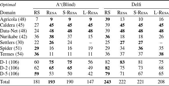
As expected, the larger the difference from the problem solved by the input plan, the harder solving the optimal repair problem. Indeed, the number of solved problems obtained by changing the initial state executing 5 random actions is always smaller than executing 2 random actions, which in turn is smaller than executing only 1 random action. While repair proves beneficial on average when the divergence from the problem solved by the input plan is limited (D-1 and D-2), our findings indicate that when such a divergence becomes high (at D-5) replanning from scratch becomes the most effective approach. We conjecture that as divergence increases, the performance gap widens: repair mechanisms attempt to reuse actions that progressively lose relevance for solving the problem, whereas replanning from scratch avoids such bias and can fully exploit the available choices.
Table 2 shows the distance between the input plan and the plans obtained by repairing w.r.t. the plans obtained by replanning. It comes with no surprise that the plan distance obtained by repairing using optimal planners is (almost) always much better than replanning. For only the termes domain and A
 $^*$
, replanning from scratch performs as well as repairing. Left side of Figure 2 shows a more detailed picture of the performance gap. The results in figure indicate that repairing leads to plans that are very often at least one order of magnitude less distant from the input plans than RS.
$^*$
, replanning from scratch performs as well as repairing. Left side of Figure 2 shows a more detailed picture of the performance gap. The results in figure indicate that repairing leads to plans that are very often at least one order of magnitude less distant from the input plans than RS.
Plan Distance Analysis. Each entry of the table corresponds to an average of the plan distances across problems solved by replanning from scratch (RS) or using Resa, S-Resa, L-Resa. Bolds are for best performers
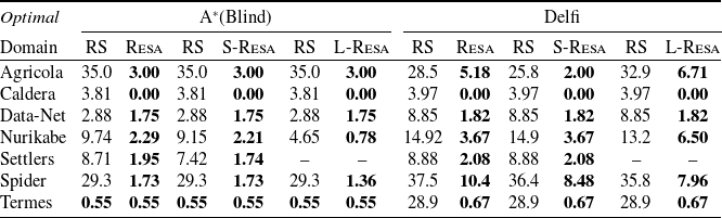
Scatter plotting the plan distances across problems solved by replanning from scratch w.r.t. repairing by Resa using the optimal (left) and the satisficing (right) planners.
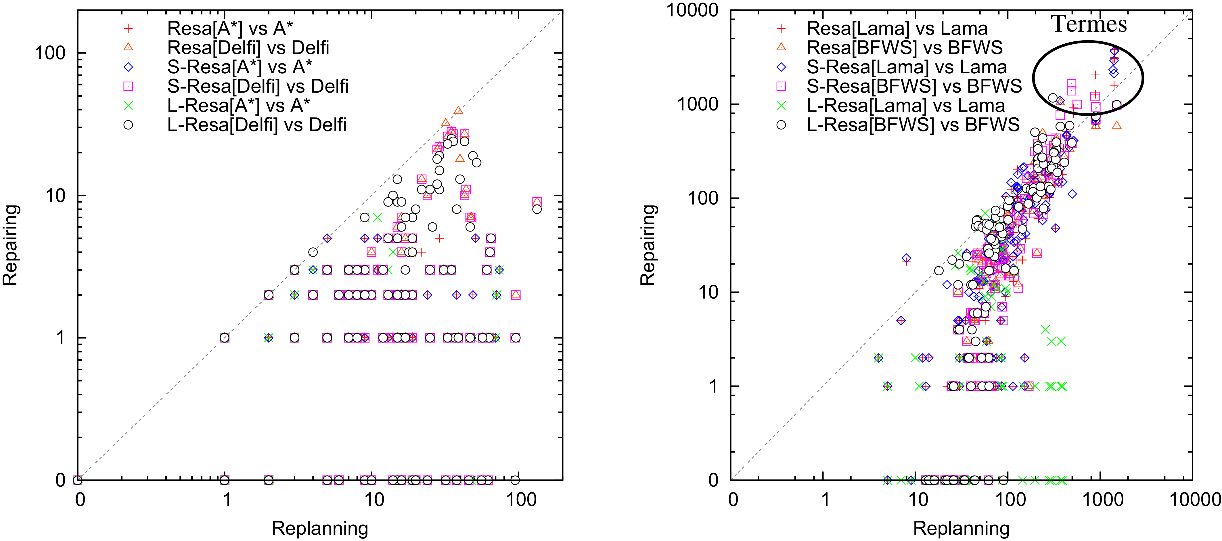
RS vs Resa, Satisficing Planning. Table 3 reports on the coverage of
 $\mathsf{Lama}$
and
$\mathsf{Lama}$
and
 $\mathsf{BFWS}$
with or without our compilations. Note that our compilations let us improve on the coverage of
$\mathsf{BFWS}$
with or without our compilations. Note that our compilations let us improve on the coverage of
 $\mathsf{Lama}$
over three domains, gets the same coverage as
$\mathsf{Lama}$
over three domains, gets the same coverage as
 $\mathsf{Lama}$
for the caldera domain, and degrades the coverage over agricola, spider and termes. For these domains, the problems have solution plans definitely longer than for other domains. Our conjecture is that longer plans make the compilation more difficult, nullifying the guidance that such plans can provide in solving the problem. The results of Resa with
$\mathsf{Lama}$
for the caldera domain, and degrades the coverage over agricola, spider and termes. For these domains, the problems have solution plans definitely longer than for other domains. Our conjecture is that longer plans make the compilation more difficult, nullifying the guidance that such plans can provide in solving the problem. The results of Resa with
 $\mathsf{BFWS}$
are similar.
$\mathsf{BFWS}$
are similar.
Coverage Analysis. Each entry of the table corresponds to the number of problems solved by the system identified by the column: replanning from scratch (RS), or using Resa, S-Resa, and L-Resa. D-{1,2,5} is a regrouping of the instances that considers all instances computed by injecting 1, 2, or 5 random actions in sequence. The number of problems is in parenthesis. Bold is for best performers
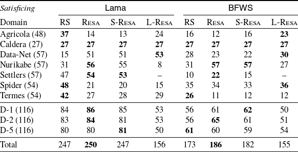
Interestingly, differently from the optimal setting, the satisficing repair planning problem does not become more difficult as the number of differences w.r.t. the problem solved by the input plan increases. Indeed, the number of solved problems obtained by changing the initial state executing 1, 2, or 5 random actions is similar.
The total number of problems solved by L-Resa is considerably lower than that achieved by RS, as well as by repairing with Resa and S-Resa. Our findings nevertheless show some complementarity among the compilations. For example, using
 $\mathsf{Lama}$
, L-Resa solves 2 problems more than Resa in Data-Net, 1 more problem in termes, and 10 problems more in Agricola. Similarly, using
$\mathsf{Lama}$
, L-Resa solves 2 problems more than Resa in Data-Net, 1 more problem in termes, and 10 problems more in Agricola. Similarly, using
 $\mathsf{BFWS}$
, L-Resa solves more problems for the Agricola, Data-Net and Spider domains. This is due to the fact that both
$\mathsf{BFWS}$
, L-Resa solves more problems for the Agricola, Data-Net and Spider domains. This is due to the fact that both
 $\mathsf{Lama}$
and
$\mathsf{Lama}$
and
 $\mathsf{BFWS}$
seem more efficient, at times, when we submit a lifted representation of the operators instead of a grounded one. It is also interesting to note that the problems compiled by L-Resa are much shorter than those compiled by Resa and S-Resa. Indeed, for our benchmark the problem representation of L-Resa is up to more than two orders of magnitude shorter.
$\mathsf{BFWS}$
seem more efficient, at times, when we submit a lifted representation of the operators instead of a grounded one. It is also interesting to note that the problems compiled by L-Resa are much shorter than those compiled by Resa and S-Resa. Indeed, for our benchmark the problem representation of L-Resa is up to more than two orders of magnitude shorter.
Table 4 shows that for all domains but termes the plans computed by Resa with both
 $\mathsf{Lama}$
and
$\mathsf{Lama}$
and
 $\mathsf{BFWS}$
are less distant from the input plan than RS. In termes, very long input plans give no fruitful information to the search. The results for S-Resa and L-Resa are similar to those for Resa. The right side of Figure 2 shows a more detailed picture about the plan distance. Repairing leads to plans that are usually less distant from the input plans and often at least one order of magnitude less distant than replanning from scratch.
$\mathsf{BFWS}$
are less distant from the input plan than RS. In termes, very long input plans give no fruitful information to the search. The results for S-Resa and L-Resa are similar to those for Resa. The right side of Figure 2 shows a more detailed picture about the plan distance. Repairing leads to plans that are usually less distant from the input plans and often at least one order of magnitude less distant than replanning from scratch.
Plan Distance Analysis. Each entry of the table corresponds to an average of the plan distances across problems solved by replanning from scratch (RS) or using Resa, S-Resa, L-Resa. Bolds are for best performers

LPG-Adapt vs Resa. This experiment evaluates the effectiveness of repairing using our approach w.r.t. using
 ${{{\mathsf{LPG}\textrm{-}\mathsf{adapt}}}}$
, the state-of-the-art for the plan repair. For our approach, we used the problems compiled using Resa, as it generally works better than S-Resa and L-Resa, and ran
${{{\mathsf{LPG}\textrm{-}\mathsf{adapt}}}}$
, the state-of-the-art for the plan repair. For our approach, we used the problems compiled using Resa, as it generally works better than S-Resa and L-Resa, and ran
 $\mathsf{Delfi1}$
and
$\mathsf{Delfi1}$
and
 $\mathsf{Lama}$
, the best performers among the used optimal and satisficing planners. Specifically, for this analysis we take the best solution found by
$\mathsf{Lama}$
, the best performers among the used optimal and satisficing planners. Specifically, for this analysis we take the best solution found by
 ${{{\mathsf{LPG}\textrm{-}\mathsf{adapt}}}}$
and Resa using
${{{\mathsf{LPG}\textrm{-}\mathsf{adapt}}}}$
and Resa using
 $\mathsf{Lama}$
in anytime modality run up to 1800 seconds.
$\mathsf{Lama}$
in anytime modality run up to 1800 seconds.
The results in Table 5 show that, for all domains but termes, Resa with
 $\mathsf{Delfi1}$
is competitive with
$\mathsf{Delfi1}$
is competitive with
 ${{{\mathsf{LPG}\textrm{-}\mathsf{adapt}}}}$
in terms of coverage, while guaranteeing the optimality of the solution for the repair problem. The plans computed by Resa with
${{{\mathsf{LPG}\textrm{-}\mathsf{adapt}}}}$
in terms of coverage, while guaranteeing the optimality of the solution for the repair problem. The plans computed by Resa with
 $\mathsf{Delfi1}$
are up to one order of magnitude closer to the input plans (i.e., in agricola). Resa with
$\mathsf{Delfi1}$
are up to one order of magnitude closer to the input plans (i.e., in agricola). Resa with
 $\mathsf{Lama}$
solves much more problems than
$\mathsf{Lama}$
solves much more problems than
 ${{{\mathsf{LPG}\textrm{-}\mathsf{adapt}}}}$
overall, but is not effective in termes where
${{{\mathsf{LPG}\textrm{-}\mathsf{adapt}}}}$
overall, but is not effective in termes where
 ${{{\mathsf{LPG}\textrm{-}\mathsf{adapt}}}}$
was able to solve many more instances. Missing results of Table 5 are due to
${{{\mathsf{LPG}\textrm{-}\mathsf{adapt}}}}$
was able to solve many more instances. Missing results of Table 5 are due to
 ${{{\mathsf{LPG}\textrm{-}\mathsf{adapt}}}}$
not supporting conditional effects.
${{{\mathsf{LPG}\textrm{-}\mathsf{adapt}}}}$
not supporting conditional effects.
Coverage and plan distance between
 ${{{\mathsf{LPG}\textrm{-}\mathsf{adapt}}}}$
and Resa using
${{{\mathsf{LPG}\textrm{-}\mathsf{adapt}}}}$
and Resa using
 $\mathsf{Delfi1}$
and
$\mathsf{Delfi1}$
and
 $\mathsf{Lama}$
over the problems derived from the optimal track of IPC-18. Bolds are for best performers; “–” for unsupported
$\mathsf{Lama}$
over the problems derived from the optimal track of IPC-18. Bolds are for best performers; “–” for unsupported

Coverage Analysis. Each entry of the table corresponds to the number of problems solved by the system identified by the column: replanning from scratch (RS), or using M-Resa with 1 (1P), 2 (2P), or 5 (5P) input plans. D-{1,2,5} is a regrouping of the instances that considers all instances computed by injecting 1, 2, or 5 random actions in sequence. The number of problems is in parenthesis. Bolds are for best performers

RS vs M-Resa, Optimal Planning In the rest of this section, we focus on evaluating the effectiveness of M-Resa. For this experiment, we considered 2 and 5 input plans.
Table 6 shows the coverage of M-Resa with a different number of input plans w.r.t. replanning from scratch. With 2 input plans, M-Resa using
 $A^\star$
solves more problems than RS for five domains over seven, while with 5 input plans M-Resa using
$A^\star$
solves more problems than RS for five domains over seven, while with 5 input plans M-Resa using
 $A^\star$
solves more problems for only three domains. The total number of problems solved by M-Resa
$A^\star$
solves more problems for only three domains. The total number of problems solved by M-Resa
 $[A^\star]$
with 2 or 5 input plans is comparable than RS. The picture is different with
$[A^\star]$
with 2 or 5 input plans is comparable than RS. The picture is different with
 $\mathsf{Delfi1}$
in place of A
$\mathsf{Delfi1}$
in place of A
 $^*$
, as M-Resa
$^*$
, as M-Resa
 $[\mathsf{Delfi1}]$
solves more problems for only 3 domains over 7. In general, the results in Table 6 indicates that the optimal multi-repair planning problem is more difficult for
$[\mathsf{Delfi1}]$
solves more problems for only 3 domains over 7. In general, the results in Table 6 indicates that the optimal multi-repair planning problem is more difficult for
 $\mathsf{Delfi1}$
than RS, while the hardness is comparable using A
$\mathsf{Delfi1}$
than RS, while the hardness is comparable using A
 $^*$
. Moreover, as expected, the greater the number of input plans, the harder the optimal multi-repair planning problem.
$^*$
. Moreover, as expected, the greater the number of input plans, the harder the optimal multi-repair planning problem.
As for the comparison in terms of plan distance, the distance of M-Resa is computed as in Definition 4; similarly, the distance of a plan obtained by replanning is the minimum between the distances from any input plan. Table 7 shows that, as expected, repairing using M-Resa with an optimal planner is always better than RS in terms of plan distance, and M-Resa sometimes computes plans that are at least one order of magnitude more similar to the input plan than RS. Replanning by
 $A^\star$
computes plans that are as far from the input plan as M-Resa only for termes domain. For the agricola domain,
$A^\star$
computes plans that are as far from the input plan as M-Resa only for termes domain. For the agricola domain,
 $A^\star$
and 5 input plans, we do not have data because the problems solved by replanning are different from those solved by repairing with M-Resa. It is not surprising to observe that, both by replanning and repairing, the distances tends to decrease w.r.t. an increasing number of input plans. Indeed, the higher the number of input plans, the more the chance to be stable with at least one of them. Left side of Figure 3 shows a more detailed picture of the plan distances obtained by repairing and replanning. Like for a single input plan, solving the optimal multi-repair problem leads to plans that are very often at least one order of magnitude less distant from the input plans than replanning from scratch.
$A^\star$
and 5 input plans, we do not have data because the problems solved by replanning are different from those solved by repairing with M-Resa. It is not surprising to observe that, both by replanning and repairing, the distances tends to decrease w.r.t. an increasing number of input plans. Indeed, the higher the number of input plans, the more the chance to be stable with at least one of them. Left side of Figure 3 shows a more detailed picture of the plan distances obtained by repairing and replanning. Like for a single input plan, solving the optimal multi-repair problem leads to plans that are very often at least one order of magnitude less distant from the input plans than replanning from scratch.
Plan Distance Analysis. Each entry of the table corresponds to an average of the plan distances across problems solved by replanning from scratch (RS) or using M-Resa with 1 (1P), 2 (2P), or 5 (5P) input plans. Bolds are for best performers
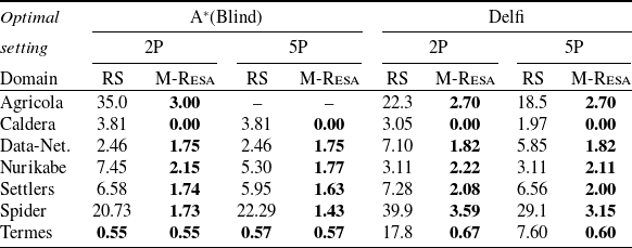
Scatter plotting the plan distances across problems solved by replanning from scratch w.r.t. repairing by M-Resa using the optimal (left) and the satisficing (right) planners.
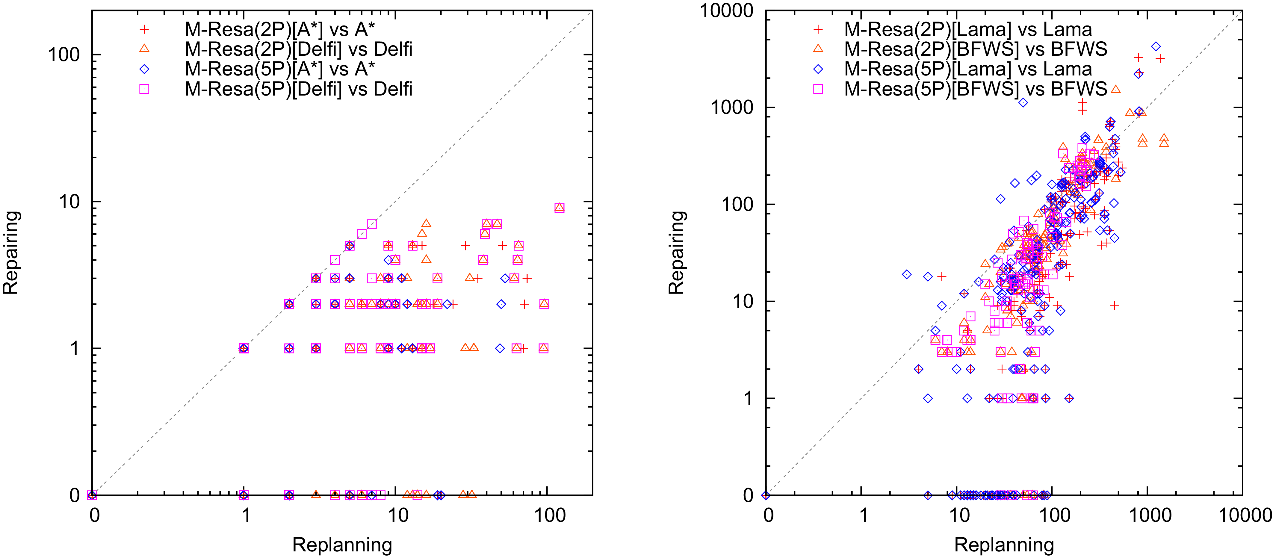
RS vs M-Resa, Satisficing Planning Table 8 shows the coverage obtained by repairing with M-Resa w.r.t. replanning with either
 $\mathsf{Lama}$
or
$\mathsf{Lama}$
or
 $\mathsf{BFWS}$
. The results in the table show that solving the multi-repair planning problem by using
$\mathsf{BFWS}$
. The results in the table show that solving the multi-repair planning problem by using
 $\mathsf{Lama}$
is slightly harder than RS, while it becomes significantly more difficult using
$\mathsf{Lama}$
is slightly harder than RS, while it becomes significantly more difficult using
 $\mathsf{BFWS}$
. As for the hardness of solving the multi-repair planning problem with a different number of input plans, we have mixed results: using
$\mathsf{BFWS}$
. As for the hardness of solving the multi-repair planning problem with a different number of input plans, we have mixed results: using
 $\mathsf{Lama}$
, solving the problems with 2 input plans is approximately as hard as with 5 input plans, while using
$\mathsf{Lama}$
, solving the problems with 2 input plans is approximately as hard as with 5 input plans, while using
 $\mathsf{BFWS}$
the hardness tends to increase with the number of input plans.
$\mathsf{BFWS}$
the hardness tends to increase with the number of input plans.
Finally, Table 9 shows the evaluation between M-Resa and RS in terms of plan distance. M-Resa with every considered number of input plans is (almost) always better than RS for all domains but termes and spider using
 $\mathsf{BFWS}$
and termes using
$\mathsf{BFWS}$
and termes using
 $\mathsf{Lama}$
. As mentioned before, the input plans for termes are very long, and we conjecture they cannot provide good guidance for the heuristics of
$\mathsf{Lama}$
. As mentioned before, the input plans for termes are very long, and we conjecture they cannot provide good guidance for the heuristics of
 $\mathsf{Lama}$
and
$\mathsf{Lama}$
and
 $\mathsf{BFWS}$
. As for the distance from the input plans w.r.t. an increasing number of input plans, the picture with the satisficing planners is less clear than with the optimal planner. We conjecture that the larger set of actions with cost greater than zero only sometimes confuses the heuristics used by
$\mathsf{BFWS}$
. As for the distance from the input plans w.r.t. an increasing number of input plans, the picture with the satisficing planners is less clear than with the optimal planner. We conjecture that the larger set of actions with cost greater than zero only sometimes confuses the heuristics used by
 $\mathsf{Lama}$
and
$\mathsf{Lama}$
and
 $\mathsf{BFWS}$
. Right side of Figure 3 shows a more detailed picture of the plan distances obtained by repairing w.r.t. replanning from scratch. The conclusion we draw from this analysis is the same as for repairing a single input plan: solving the multi-repair planning problem leads to plans that are usually less distant from the input plans, and often at least one order of magnitude less distant than replanning from scratch.
$\mathsf{BFWS}$
. Right side of Figure 3 shows a more detailed picture of the plan distances obtained by repairing w.r.t. replanning from scratch. The conclusion we draw from this analysis is the same as for repairing a single input plan: solving the multi-repair planning problem leads to plans that are usually less distant from the input plans, and often at least one order of magnitude less distant than replanning from scratch.
8. Related work
Sooner or later plans will fail regardless on how precise the models are. This observation has led many researchers to question on how to build intelligent agents that can deal with this issue. One possibility is to anticipate everything upfront and therefore build on models that take the uncertainty into account from the very beginning, assuming or not observation capabilities of the agent (Cimatti et al., Reference Cimatti, Pistore, Roveri and Traverso2003; Rintanen, Reference Rintanen2004; Grastien & Scala, Reference Grastien and Scala2020), and whether the agent has some probability distribution over the state space, and action effects (Kaelbling et al., Reference Kaelbling, Littman and Cassandra1998). However, it is in many cases much more practical to revise the plan as soon as the actual discrepancy from the plan being executed is observed (Ingrand & Ghallab, Reference Ingrand and Ghallab2017).
Coverage Analysis. Each entry of the table corresponds to the number of problems solved by the system identified by the column: replanning from scratch (RS), or using M-Resa with 1 (1P), 2 (2P), or 5 (5P) input plans. D-{1,2,5} is a regrouping of the instances that considers all instances computed by injecting 1, 2, or 5 random actions in sequence. The number of problems is in parenthesis. Bolds are for best performers

Plan Distance Analysis. Each entry of the table corresponds to an average of the plan distances across problems solved by replanning from scratch (RS) or using M-Resa with 1 (1P), 2 (2P), or 5 (5P) input plans. Bolds are for best performers
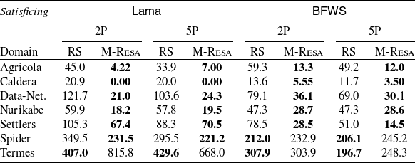
One possibility is replanning (e.g., desJardins et al., 1999; Yoon et al., Reference Yoon, Fern and Givan2007; Borrajo & Veloso, Reference Borrajo, Veloso, Biundo, Do, Goldman, Katz, Yang and Zhuo2021; Cardellini et al., Reference Cardellini, Dodaro, Galatà, Giardini, Maratea, Nisopoli and Porro2023; Pozanco et al., Reference Pozanco, Borrajo and Veloso2023), the other is trying to re-use as much as possible the old plan by repairing it (e.g., van der Krogt & de Weerdt, Reference van der Krogt and de Weerdt2005; Fox et al., Reference Fox, Gerevini, Long and Serina2006; Garrido et al., Reference Garrido2010; Gerevini & Serina, Reference Gerevini and Serina2010; Scala, Reference Scala2014; Scala & Torasso, Reference Scala and Torasso2014; Percassi et al., Reference Percassi, Scala and Vallati2023). This paper focuses on repair, and because of this in what follows we provide a small outlook to those works which we believe are relevant to what we studied here. van der Krogt and de Weerdt (Reference van der Krogt and de Weerdt2005) define repair as a two-step process: first, the flawed actions are removed (unrefinement), then new actions are added to fix the gaps. The algorithm searches for solutions in the plan space and backtracks to the unrefinement stage if no solution is found during refinement. Gerevini and Serina (Reference Gerevini and Serina2010) look for ‘windows’ of plans that need to be fixed, and runs planning off-the-shelf only over those portions. Other approaches, somehow closer to our approach, look instead at compilation techniques. Scala and Torasso (Reference Scala and Torasso2014) compile the repair problem as a Constraint Satisfaction Problem over the space of action modalities. This work also is motivated by stability to some extent, though stability is controlled by focusing the search on a specific portion of the state space. Other compilation-based approach is presented by Percassi et al. (Reference Percassi, Scala and Vallati2023) and Scala (Reference Scala2014). Specifically, Percassi et al. (Reference Percassi, Scala and Vallati2023) propose a repair technique based on fixing the timing of the actions and does so by reformulating a time-discrete PDDL+ problem. Scala (Reference Scala2014) instead proposes the use of macro-operators as a means to re-use previous portions of the plans. Scala and Torasso (Reference Scala and Torasso2015) extend their previous work to extract macros from plan decompositions obtained through a process of deordering.
The state-of-the art approach to plan repair prior to this work was
 ${{{\mathsf{LPG}\textrm{-}\mathsf{adapt}}}}$
(Fox et al., Reference Fox, Gerevini, Long and Serina2006).
${{{\mathsf{LPG}\textrm{-}\mathsf{adapt}}}}$
(Fox et al., Reference Fox, Gerevini, Long and Serina2006).
 $\mathsf{LPG}$
(Gerevini et al., Reference Gerevini, Saetti and Serina2011) is a planner that natively supports plan repair, as it does plan search by refinement, making repair a byproduct of the planner’s search process. The extension into
$\mathsf{LPG}$
(Gerevini et al., Reference Gerevini, Saetti and Serina2011) is a planner that natively supports plan repair, as it does plan search by refinement, making repair a byproduct of the planner’s search process. The extension into
 ${{{\mathsf{LPG}\textrm{-}\mathsf{adapt}}}}$
(Fox et al., Reference Fox, Gerevini, Long and Serina2006) makes the repair more central, and also introduces the plan distance metric that we use in this paper. All these works do not however focus on producing optimal stable plans; this paper presents the first approach to bridge this gap systematically by compilation.
${{{\mathsf{LPG}\textrm{-}\mathsf{adapt}}}}$
(Fox et al., Reference Fox, Gerevini, Long and Serina2006) makes the repair more central, and also introduces the plan distance metric that we use in this paper. All these works do not however focus on producing optimal stable plans; this paper presents the first approach to bridge this gap systematically by compilation.
The compilation path that we use is similar in the spirit to the compilation proposed by Keyder and Geffner (Reference Keyder and Geffner2009), in which one can see the process of repair as an oversubscription problem where the goals of the problem remain the same but we seek for those plans which minimize the distance to the previous one(s). Similar is also the technique that attributes cost only to those actions which signal the fact that some over-subscribed goal is not reachable. In our case this over-subscribed goals are the actions from the original plan that we did not cover, or those actions that we added to achieve the (sub)goals but were not in the original plan.
Researchers also looked at the problem of repairing plans using domain-specific knowledge, like hierarchical task networks. A research direction about plan repair via HTN focuses on the plan generation process. That is, several approaches propose algorithms that directly revise plan generation by first retracting the development steps responsible for the failed plan fragments, for example, Bidot et al. (Reference Bidot, Schattenberg and Biundo2008), Boella and Damiano (Reference Boella, Damiano and Scott2002), Warfield et al. (Reference Warfield, Hogg, Lee-Urban and Muñoz-Avila2007). The most recent approach among those we are aware of is ShopFixer (Goldman et al., Reference Goldman, Kuter and Freedman2020), which uses a graph of causal links and task decomposition to identify the portion of the plan to repair. In particular, it finds the minimal subtree of the plan tree that contain an unsupported precondition; then, it restarts the search by backjumping to the corresponding entry in the search tree, and updates the world state with the effects of the disturbance. Another research direction is based on the compilation of the HTN problem to enforce HTN plans to start with a prefix of actions (e.g., Bercher et al., Reference Bercher, Biundo, Geier, Hoernle, Nothdurft, Richter and Schattenberg2014). A recent compilation approach was proposed by Höller et al. (Reference Höller, Bercher, Behnke and Biundo2020). In addition to new propositions and actions, their compilation introduces new primitive and abstract taks into the problem definition, so that the HTN planning system is forced to generate a solution that starts with the prefix of the plan executed before an unexpected change. Our approach is different in the scope, as it does not require a task decomposition network and can be used to compute plans as stable as possible w.r.t. an input plan.
9. Conclusion
This paper faces the problem of optimal plan repair, which consists in finding a plan that solves the problem and also minimizes the distance between the solution plan and the input plan. We solved this problem through a compilation into classical planning. On top of that, we showed that it is possible to obtain an easy extension of this approach that takes multiple plans into account, therefore minimizing the distance over such a set. For the case with a single plan, we also provide some additional compilation schemes, including a lifted encoding – no need to ground upfront which provides some further complementary behavior.
Our results show that not only is this approach possible but also competitive with
 ${{{\mathsf{LPG}\textrm{-}\mathsf{adapt}}}}$
, the state-of-the-art system for repairing plans, while can also guarantee that the plan stability is optimised. As a future work we want to investigate different metrics for stability and adaptations of Resa to such metrics. Moreover, it would be interesting to use this approach for other settings, such as numeric or temporal planning (Fox & Long, Reference Fox and Long2003). Numeric planning problems could easily leverage this compilation schema, particularly since the use of numerical functions would significantly reduce the number of actions required by the compilation, while temporal planning would require a more profound restructuring of the encoding.
${{{\mathsf{LPG}\textrm{-}\mathsf{adapt}}}}$
, the state-of-the-art system for repairing plans, while can also guarantee that the plan stability is optimised. As a future work we want to investigate different metrics for stability and adaptations of Resa to such metrics. Moreover, it would be interesting to use this approach for other settings, such as numeric or temporal planning (Fox & Long, Reference Fox and Long2003). Numeric planning problems could easily leverage this compilation schema, particularly since the use of numerical functions would significantly reduce the number of actions required by the compilation, while temporal planning would require a more profound restructuring of the encoding.
Competing interests
The authors declare none.


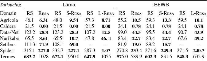
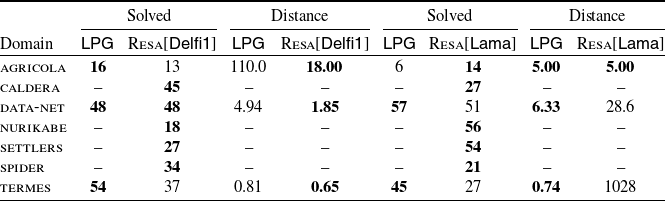


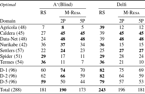


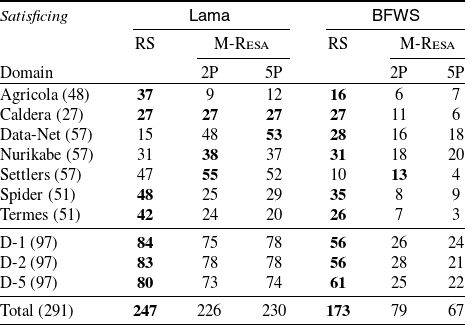


 Open access